Two Degree of Freedom Free Vibration

Abstract

Let’s extend our free vibration analysis from Chap. 2 to include two degrees of freedom in the model. This would make sense, for example, if we completed a measurement to determine the frequency response function (FRF) for a system and saw that there were obviously two modes of vibration within the frequency range of interest; see Fig. 4.1.

Exercises

• 1. Given the eigenvalues and eigenvectors for the two degree of freedom system shown in Fig. P4.1, determine the modal matrices m _q (kg), c _q (N-s/m), and k _q (N/m).

  $$ {s_{{1}}}^{{2}} = - {1} \times {1}{0^{{6}}}{\hbox{rad}}/{{\hbox{s}}^{{2}}} $$
  $$ {s_{{2}}}^{{2}} = - {7} \times {1}{0^{{6}}}{\hbox{rad}}/{{\hbox{s}}^{{2}}} $$
  $$ \begin{array}{lllll}{{\psi_1} = \left\{ \begin{array}{lllll}{0.5} \\1 \\\end{array} \right\}} & {{\psi_2} = \left\{ \begin{array}{lllll}{ - 2.5} \\1 \\\end{array} \right\}} \\\end{array} $$

  Fig. P4.1

  

  Two degree of freedom spring-mass-damper system

• 2. Given the two degree of freedom system in Fig. P4.2, complete the following.

  • (a) Write the equations of motion in matrix form.

  • (b) Write the system characteristic equation using Laplace notation. Your solution should be a polynomial that is quadratic in s ² with appropriate numerical coefficients.

  • (c) Calculate the natural frequencies (in Hz).

  • (d) Determine the two mode shapes (normalize to coordinate x ₁).

  Fig. P4.2

  

  Two degree of freedom spring-mass system

• 3. Given the two degree of freedom system shown in Fig. P4.3, complete the following.

  Fig. P4.3

  

  Two degree of freedom spring-mass system

  • (a) Write the equations of motion in matrix form.

  • (b) Write the system characteristic equation using Laplace notation. Your solution should be a polynomial that is quadratic in s ² with appropriate numerical coefficients.

  • (c) Determine the natural frequencies (in rad/s).

  • (d) Determine the mode shapes (normalize to coordinate x ₂).

• 4. A two degree of freedom spring-mass system is shown in Fig. P4.4. For harmonic free vibration, complete the following if k = 5 × 10⁶ N/m and m = 2 kg.

  Fig. P4.4

  

  Two degree of freedom spring-mass system

  • (a) Draw the free body diagram showing the forces on the two masses during vibration.

  • (b) Write the two equations of motion in matrix form. First show the equations symbolically and then substitute the numerical values for m and k.

  • (c) Write the characteristic equation for this system. First show the equation symbolically and then substitute the numerical values for m and k.

  • (d) Determine the numerical roots of the characteristic equation (which is quadratic in s²). What do these two roots represent?

  • (e) Determine the two mode shapes for this system. Normalize the mode shapes to coordinate x ₁.

  Fig. P4.5

  

  Two degree of freedom spring-mass system

• 5. A two degree of freedom spring-mass system is displayed in Fig. P4.5. For harmonic free vibration, complete the following if k ₁ = 2 × 10⁶ N/m, m ₁ = 0.8 kg, k ₂ = 1 × 10⁶ N/m, and m ₂ = 1.4 kg. The initial displacements for the system’s free vibration are x ₁(0) = 2 mm and x ₂(0) = 1 mm and the initial velocities are ${\dot{x}_1}(0) = 0\;{\hbox{mm/s}}$ and ${\dot{x}_2}(0) = 5\;{\hbox{mm/s}}$.

  • (a) Calculate the two natural frequencies and mode shapes. Normalize the mode shapes (eigenvectors) to coordinate x ₂.

  • (b) Define the modal matrix and determine the modal mass and stiffness matrices.

  • (c) Write the uncoupled single degree of freedom time responses for the modal coordinates q ₁ and q ₂. Use the following form: ${q_{{1,2}}}(t) = {A_{{1,2}}}\cos \left( {{\omega_{{{n_{{1,2}}}}}}t} \right) + {B_{{1,2}}}\sin \left( {{\omega_{{{n_{{1,2}}}}}}t} \right)$ with units of mm.

  • (d) Write the time responses for the local coordinates x ₁ and x ₂ (in mm).

  • (e) Plot the time responses for x ₁ and x ₂ (in mm). Define the time vector as: t = 0:0.0001:0.2; (in seconds).

• 6. For the same system as described in problem 5, complete the following.

  • (a) The initial displacements for the system’s free vibration are x ₁(0) = 0.378 mm and x ₂(0) = 1 mm and the initial velocities are ${\dot{x}_1}(0) = 0\;{\hbox{mm/s}}$ and ${\dot{x}_2}(0) = 0\;{\hbox{mm/s}}$. Plot the time responses for x ₁ and x ₂ (in mm). Define the time vector as: t = 0:0.0001:0.2; (in seconds). What is the vibrating frequency for both ${x_1}(t)$ and ${x_2}(t)$? What is special about these initial conditions to give this result?

  • (b) The initial displacements for the system’s free vibration are x ₁(0) = −4.628 mm and x ₂(0) = 1 mm and the initial velocities are ${\dot{x}_1}(0) = 0\;{\hbox{mm/s}}$ and ${\dot{x}_2}(0) = 0\;{\hbox{mm/s}}$. Plot the time responses for x ₁ and x ₂ (in mm). Define the time vector as: t = 0:0.0001:0.2; (in seconds). What is the vibrating frequency for both ${x_1}(t)$ and ${x_2}(t)$? What is special about these initial conditions to give this result?

• 7. A two degree of freedom spring-mass-damper system is shown in Fig. P4.7. For harmonic free vibration, complete the following if k ₁ = 2 × 10⁵ N/m, c ₁ = 60 N-s/m, m ₁ = 2.5 kg, k ₂ = 5.5 × 10⁴ N/m, c ₂ = 16.5 N-s/m, and m ₂ = 1.2 kg.

  Fig. P4.7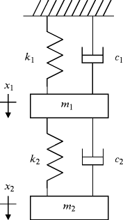

  

  Two degree of freedom spring-mass-damper system under free vibration

  • (a) Verify that proportional damping exists.

  • (b) Define the modal matrix and determine the modal mass, stiffness, and damping matrices. Normalize the mode shapes to coordinate x ₂.

• 8. Given the two degree of freedom system in Fig. P4.8, complete the following.

  Fig. P4.8

  

  Two degree of freedom spring-mass system

  • (a) Write the equations of motion in matrix form.

  • (b) Verify that proportional damping exists.

  • (c) Determine the roots of the characteristic equation. What do these roots represent?

  • (d) Determine the two mode shapes (normalize to coordinate x ₁).

• 9. Determine the mass, damping, and stiffness matrices in local coordinates for the model shown in Fig. P4.9.

  Fig. P4.9

  

  Three degree of freedom spring-mass-damper model

• 10. Given the mass, damping, and stiffness matrices for the model shown in Fig. P4.9 determined from problem 9, can proportional damping exist for this system? Justify your answer.