Sememe-Based Lexical Knowledge Representation Learning

Abstract

Linguistic and commonsense knowledge bases describe knowledge in formal and structural languages. Such knowledge can be easily leveraged in modern natural language processing systems. In this chapter, we introduce one typical kind of linguistic knowledge (sememe knowledge) and a sememe knowledge base named HowNet. In linguistics, sememes are defined as the minimum indivisible units of meaning. We first briefly introduce the basic concepts of sememe and HowNet. Next, we introduce how to model the sememe knowledge using neural networks. Taking a step further, we introduce sememe-guided knowledge applications, including incorporating sememe knowledge into compositionality modeling, language modeling, and recurrent neural networks. Finally, we discuss sememe knowledge acquisition for automatically constructing sememe knowledge bases and representative real-world applications of HowNet.

10.1 Introduction

In the field of NLP, a series of meaningful linguistic units are generally studied, including words, phrases, sentences, discourses, and documents. Specifically, words are typically treated as the smallest usage units since they are deemed as the smallest meaningful objects which can stand by themselves. In fact, word meanings can be further split into smaller components. For instance, the meaning of the word teacher comprises the meanings of education, occupation, and teach. From the perspective of linguistics, the minimum indivisible units of meaning are defined as sememes [10].

Linguists contend that the meanings of all the words comprise a closed set of sememes, and the semantic meanings of these sememes are orthogonal to each other. Compared with words, sememes are fairly implicit, and the full set of sememes is difficult to define, not to mention how to decide which sememes a word has. To understand the human language from a finer-grained perspective, it is necessary to fathom the nature of sememe and its connection with words.

To this end, some linguists spend many years identifying sememes from both linguistic knowledge bases (KBs) and dictionaries and labeling each word with sememes, in order to construct sememe-based linguistic KBs. HowNet [23] is the most representative sememe-based linguistic KB. Besides being a linguistic KB, HowNet also contains commonsense knowledge and can be used to unveil the relationships among concepts [23].

In the following sections, we first briefly introduce backgrounds of typical linguistic KB (WordNet) and commonsense KB (ConceptNet), and then we detailedly introduce basic concepts and construction principles of HowNet, as well as the linguistic knowledge and commonsense knowledge in HowNet. Then we discuss how to represent sememe knowledge using neural networks. After that, we introduce sememe-guided NLP techniques, including how to incorporate sememe knowledge into compositionality modeling, language modeling, and recurrent neural networks. Finally, we discuss automatic knowledge acquisition for HowNet and the application of HowNet. Since most of the research (especially the research related to deep learning) in this area is conducted by our group, we will mainly take our works as examples to elaborate on the powerful capability of sememe knowledge. To provide a more comprehensive description, our discussion of the specific methods in this chapter will be more detailed.

10.2 Linguistic and Commonsense Knowledge Bases

Over the years, many human-annotated KBs have been proposed, among which linguistic KBs and commonsense KBs are the most representative ones. Serving as important lexical resources, all of these KBs have pushed forward the understanding of human language and achieved many successes in NLP applications. In this section, we first elaborate on a representative linguistic KB, WordNet, and a commonsense KB, ConceptNet, and then we discuss the unique characteristics of HowNet compared with them.

10.2.1 WordNet and ConceptNet

WordNet and ConceptNet are the most representative KBs aiming at organizing linguistic knowledge and commonsense knowledge, respectively. Both of them have shown importance in various NLP applications. We briefly give an introduction to the construction of both KBs as follows.

WordNet

WordNet [48] is a large lexical database and can also be viewed as a KB containing multi-relational data. It was first created in 1985 by George Armitage Miller, a psychology professor in the Cognitive Science Laboratory of Princeton University. Up till now, WordNet has become the most popular lexicon dictionary in the world and has been widely applied in various NLP tasks.

Based on meanings, WordNet groups English nouns, verbs, adjectives, and adverbs into synsets (i.e., sets of cognitive synonyms), which represent unique concepts. Each synset is accompanied by a brief description. In most cases, there are several short sentences illustrating the usage of words in this synset. The synsets and words are linked by conceptual-semantic and lexical relations, covering all WordNet’s 117, 000 synsets. For example, (1) the words in the same synset are linked with the synonymy relation, which indicates that these words share similar meanings and could be replaced by each other in some contexts; (2) the hypernymy/hyponymy links a general synset and a specific synset, which indicates that the specific synset is a sub-class of the general one, and (3) the antonymy describes the relation among adjectives with opposite meanings.

ConceptNet

Besides linguistic knowledge, commonsense knowledge (generic facts about social and physical environments) is also important for general artificial intelligence. ConceptNet [72] is one of the largest freely available commonsense knowledge bases. ConceptNet was first constructed in 2002 in the project of Open Mind Common Sense and was frequently updated in the following years. Like other commonsense knowledge bases, ConceptNet describes the conceptual relations among words. Nodes in ConceptNet are represented as free-text descriptions, and edges stand for symmetric relations like SimilarTo or asymmetric relations like MadeOf.

Thanks to diverse building sources and continual updating, ConceptNet has grown as the largest free commonsense KB that includes more than 21 million edges and 8 million nodes [72]. In addition, ConceptNet supports a variety of languages. Similar to other KBs, ConceptNet can be used to enhance the ability of neural networks on downstream tasks that require commonsense reasoning. Especially with the novel relation ExternalURL, ConceptNet nodes can be easily linked with nodes in other knowledge bases such as WordNet. This capability makes it more convenient to integrate commonsense knowledge and linguistic knowledge for researchers.

10.2.2 HowNet

The above-mentioned KBs take words (WordNet) or concepts (ConceptNet) as basic elements and consist of word-level or concept-level relations. Different from both KBs, HowNet treats sememes as the smallest linguistic objects and additionally focuses on the relation between sememes and words. This is one of the core differences between the design philosophy of HowNet and other KBs.

Construction of HowNet

We introduce three components for HowNet construction: (1) Sememe set construction: the sememe set is determined by analyzing, merging, and sifting the semantics of a great number of Chinese characters and words. Each sememe in HowNet is expressed by a term or a phrase in both English and Chinese to avoid ambiguity. For instance, (human | {人 }) and (ProperName | {专 }). All the sememes can be categorized into seven types, including part, attribute, attribute value, thing, space, time, and event; (2) Sememe-sense-word structure definition: considering the polysemy, HowNet annotates different sets of sememes for different senses of a word, with every sense described in both Chinese and English. Every sense is defined as the root of a “sememe tree.” For the sememes belonging to a specific sense, HowNet annotates the relations among these sememes (dubbed as “dynamic roles”). Such relations are the edges of the “sememe tree.” We illustrate an example for a word apple in Fig. 10.1, where the word apple has four senses including apple(tree), apple(phone), apple(computer), and apple(fruit); (3) Annotation process: HowNet is constructed by manual annotation of human experts. HowNet was originally built by Zhendong Dong and Qiang Dong in the 1990s and has been frequently updated ever since then, with the latest version of HowNet published in January 2019.

Fig. 10.1

An example of a word annotated with sememes in HowNet

Uniqueness of HowNet

The aforementioned KBs share several similarities, for instance, all of them are (1) structured with relational semantic networks, (2) based on the form of natural language, (3) constructed with extensive human labeling, etc. In spite of all these similarities, HowNet owns unique characteristics that differ from WordNet and ConceptNet in construction principles, design philosophy, and foci, which are discussed in the following paragraphs.

Comparison Between HowNet and WordNet

As shown in Fig. 10.2, compared with WordNet, HowNet is unique reflected in the following facets:

Fig. 10.2

Comparison between WordNet and HowNet. WordNet is based on synsets and their semantic relations, while HowNet investigates sememes and focuses on their relations to word senses. Here we discriminate characters (字 ) and words (词 ) in Chinese, with the former being smaller components for the latter

 

• 1. Basic unit and design philosophy. In human language, words are generally considered as the smallest usage units, while sememes are viewed as the smallest semantic units. Adhering to reductionism, HowNet considers sememes as the smallest objects and focuses on the relation between words and sememes; instead, the basic block of WordNet is a synset consisting of all the words expressing a specific concept; thus the design of WordNet resembles that of a thesaurus. This is the core difference between the design philosophy of HowNet and WordNet. In addition, according to Kim et al. [39], WordNet is differential by nature: instead of explicitly expressing the meaning of a word, WordNet differentiates word senses by placing them into different synsets and further assigning them to different positions in its ontology. Conversely, HowNet is constructive, i.e., exploiting sememes from a taxonomy to represent the meaning of each word sense. It is based on the hypothesis that all concepts can be reduced to relevant sememes.

• 2. Construction principle. WordNet is organized according to semantic relations among word meanings. Since word meanings can be represented by synsets, semantic relations can be treated as pointers among synsets. The taxonomy of WordNet is designed not to capture common causality or function, but to show the relations among existing lexemes [39]. Differently, the basic construction principle of HowNet is to form a networked knowledge system of the relations among concepts and the relation between attributes and concepts. Besides, HowNet is constructed using top-down induction: the ultimate sememe set is established by observing and analyzing all the possible basic sememes. After that, human experts evaluate whether every concept can be composed of the subsets of the sememe set.

• 3. Application scope. Initially designed as a thesaurus, WordNet gradually evolved into a self-contained machine-readable dictionary of semantics. In contrast, HowNet is established towards building a computer-oriented semantic network [22]. In addition, one advantage of WordNet is that it supports multiple languages. For example, since many countries have established lexical databases based on WordNet, it can be easily applied to cross-lingual scenarios. However, since HowNet mainly supports English and Chinese, most of its applications are bilingual. In fact, we have also proposed methods to automatically build sememe KBs for other languages, which will be discussed later.

Comparison Between HowNet and ConceptNet

HowNet and ConceptNet differ from each other in the following aspects:

• 1. Coverage of commonsense knowledge. The commonsense knowledge contained in ConceptNet is relatively explicit, partly because the nodes in ConceptNet are represented as free-text descriptions. In contrast, the notions of nodes in HowNet are purely lexical items (e.g., word senses and sememes with atomic meanings), which correspond to more rock-bottom commonsense knowledge. Therefore, the commonsense knowledge of HowNet is more implicit. For instance, from ConceptNet, we know directly that the concept buy book is related to the concept a bookstore because the former is a subevent of the latter, while in HowNet, we learn such information by simple induction and reasoning: the word bookstore is associated with sememes publication and buy, and the word book consists of the sememe publication. Similarly, numerous generic facts about the world can be derived from HowNet. We contend that despite the implicit nature of commonsense knowledge, HowNet actually covers more diverse facets of the world facts than ConceptNet.

• 2. Foci and construction principle. ConceptNet focuses on everyday episodic concepts and the semantic relations among compound concepts, which are organized hierarchically. These high-level concepts can be contributed by every ordinary person. In contrast, HowNet focuses on rock-bottom linguistic and conceptual knowledge of the human language, and its annotation requires the basic understanding of sememe hierarchy. The above distinction leads to different construction methods for both KBs. HowNet is constructed solely by human handcrafting of linguistic experts, whereas the construction of ConceptNet involves the general public without much background knowledge. In consequence, the annotation of HowNet has higher quality than ConceptNet by nature.

• 3. Application scope. HowNet annotates sememes for each word sense and thus differentiates different word meanings. Nevertheless, the concepts and relations annotated in ConceptNet may be ambiguous. The ambiguous nature of ConceptNet could hinder it from being directly leveraged in NLP applications, such as word sense disambiguation. In contrast, the sememe knowledge of HowNet can be more easily incorporated into modern neural networks since HowNet overcomes the problem of word ambiguity.

OpenHowNet

To help researchers get access to HowNet data in an easier way, encouraged and approved by the inventors of HowNet, Zhendong Dong and Qiang Dong, we have created OpenHowNet¹ (Fig. 10.3). OpenHowNet is a free open-source sememe KB, which comprises the core data of HowNet. There are two core components of OpenHowNet, i.e., OpenHowNet Web and OpenHowNet API:

• 1. OpenHowNet Web gives a comprehensive description of HowNet, including statistics of OpenHowNet dataset, research articles relevant to sememe knowledge, history of HowNet, etc. With OpenHowNet, users can easily understand the basic idea of sememe and get familiar with advanced research topics of HowNet. Besides, OpenHowNet supports the visualization of the sememe tree for each sense in HowNet. Together with the tree structure, OpenHowNet Web provides additional information, such as the POS tags, the plain text form of the sememe tree, and semantically related senses. This capability makes it easier for users to understand the core linguistic information of each word sense. We also link OpenHowNet to representative KBs such as BabelNet and ConceptNet, which makes it easier for users to get access to information of each word sense outside HowNet.

  Fig. 10.3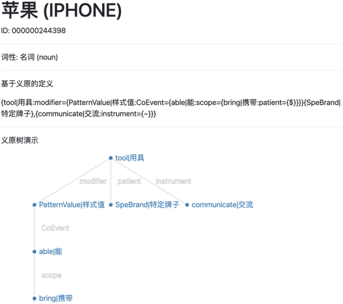

  

  A snapshot of the OpenHowNet website

• 2. OpenHowNet API supports some important functionalities, e.g., visualizing the sememe tree of a sense, searching senses or sememes, computing word similarity based on sememe tree annotation, etc. We believe such a toolkit can help researchers leverage the sememe annotation in HowNet more easily.

In summary, armed with OpenHowNet, it will be more convenient for beginners to get familiar with the design philosophy of HowNet, easier for senior researchers to utilize the sememe knowledge, and handier for industrial practitioners to deploy their HowNet applications. You can also read our research paper about OpenHowNet [64] for more details.

10.2.3 HowNet and Deep Learning

Back in the early era when statistical learning dominates mainstream NLP techniques, linguistic and commonsense KBs are generally leveraged to provide shallow and primitive information. Typical applications include word similarity calculation [43, 55], word sense disambiguation [3, 85], etc. Ever since the emergence of deep learning, HowNet has renewed a surge of interest in both academic and industrial communities, reflected in the significant proliferation of related research papers. Assisted by the powerful representation capability of deep learning, HowNet is endowed with more imaginative usage to fully exploit its knowledge. Before delving into the usage of sememe knowledge, we introduce several advantages of HowNet.

Advantages of HowNet

The sememe knowledge of HowNet owns unique advantages over other linguistic KBs in the era of deep learning, reflected in the following characteristics:

• 1. In terms of natural language understanding, sememe knowledge is closer to the characteristics of natural language. The sememe annotation breaks the lexical barrier and offers an in-depth understanding of the rich semantic information behind the vocabulary. Compared with other KBs that can only be applied to the word level or the sense level, HowNet provides finer-grained linguistic and commonsense information.

• 2. Sememe knowledge turns out to be a natural fit for deep learning techniques. By accurately depicting semantic information through a unified sememe labeling system, the meaning of each sememe is clear and fixed and thus can be naturally incorporated into the deep learning model as informative labels/tags of words. As we will show later, most of the modern NLP models are built on word sequences. It is natural and convenient to directly extract the information for each word from HowNet to leverage its knowledge.

• 3. Sememe knowledge can mitigate poor model performance in low-resource scenarios. Since the sememe set is carefully pre-defined and the total number of sememes is limited, even when there only exists limited supervision, the representations of sememes can still be fully optimized. In contrast, considering the massive word representations needed to be learned, it is generally hard to learn excellent word embeddings, especially for those infrequent words. Thus the well-trained sememe representations can alleviate the problem of insufficient training and enrich the semantic meanings of words in low-resource settings.

How to Incorporate Sememe Knowledge

After showing the uniqueness and advantages of HowNet, we briefly introduce several ways (categorized according to Chap. 9) of leveraging sememe knowledge for deep learning techniques:

• 1. Knowledge augmentation. The first way targets at adding sememe knowledge into the input of neural networks or designing special neural modules that can be inserted into the original networks. In this way, the sememe knowledge can be incorporated explicitly without changing the neural architectures. Since sememes are smaller units of word senses, they always appear together with words. For instance, we can first learn sememe embeddings and directly leverage them to enrich the semantic information of word embeddings.

• 2. Knowledge reformulation. The second method for incorporating sememe knowledge is to change the original word-based model structures into sememe-based ones. A possible solution is to assign sememe experts in the neural networks. The introduction of sememe experts could properly guide neural models to produce inner hidden representations with rich semantics in a more linguistically informative way.

• 3. Knowledge regularization. The third way is to design a new training objective function based on sememe knowledge or to use knowledge as extra predictive targets. For instance, we can first extract linguistic information (e.g., the overlap of annotated sememes of different words) from HowNet and then treat it as auxiliary regularization supervision. This approach does not require modifying the specific model architecture but only introduces an additional training objective to regularize the original optimization trajectory.

In the above paragraphs, we only present the high-level ideas for sememe knowledge incorporation. In the next few sections, we will elaborate on these ideas with specific examples to showcase the powerful capabilities of HowNet and its comprehensive applications in NLP.

10.3 Sememe Knowledge Representation

To leverage sememe knowledge, we should first learn to represent it. Sememes do not exist naturally but are labeled by human experts on word senses. We can represent them using techniques similar to word representation learning (WRL). In this section, we first elaborate on how to learn sememe embeddings by representing words as a combination of sememes, and then we introduce how to incorporate sememe knowledge to better learn word representations. The introduction of this section is based on our research works [53, 62].

10.3.1 Sememe-Encoded Word Representation

WRL is a fundamental technique in many NLP tasks such as neural machine translation [75] and language modeling [6]. Many works have been proposed for learning better word representations, among which word2vec [46] strikes an excellent balance between effectiveness and efficiency. Later works propose to leverage existing KBs (such as WordNet [17] and HowNet [74]) to improve word representation.

We first introduce our sememe-encoded word representation learning (SE-WRL) [53]. SE-WRL assumes each word sense is composed of sememes and conducts word sense disambiguation according to the contexts. In this way, we could learn representations of sememes, senses, and words simultaneously. Moreover, SE-WRL proposes an attention-based method to choose an appropriate word sense according to contexts automatically. In the following paragraphs, we introduce three different variants for SE-WRL. For a word w, we denote S^(w) as its sense set. $S^{(w)} = \{s_1^{(w)}, \cdots , s_{|S^{(w)}|}^{(w)}\}$ may contain multiple senses. For each sense $s_i^{(w)}$, we denote $X_i^{(w)} = \{x_1^{(s_i)}, \cdots , x_{|X_i^{(w)}|}^{(s_i)}\}$ as the sememe set for this sense, with ${\mathbf {x}}_j^{(s_i)}$ being the embedding for the correspond sememe $x_j^{(s_i)}$.

Skip-Gram Model

Since SE-WRL extends from the skip-gram of word2vec [46], we first give a brief introduction to the skip-gram model. For a series of words {w₁, ⋯ , w_N}, the model targets at maximizing the probability of contextual words based on a centered word w_c. Specifically, we minimize the following loss (more details could be found in Chap. 2):

$$\displaystyle \begin{aligned} \begin{gathered} \mathcal{L}=-\sum_{c=l+1}^{n-l}\sum_{\substack{-l\leq k \leq l ,k\neq 0}}\log P(w_{c+k}|w_c), \end{gathered} \end{aligned} $$

(10.1)

where l is the size of the sliding window and P(w_c+k|w_c) stands for the predictive probability of the context word w_c+k conditioned on the centered word w_c. Denoting V  as the vocabulary, the probability is formalized as follows:

$$\displaystyle \begin{aligned} \begin{gathered} P(w_{c+k}|w_c) = \frac{\exp({\mathbf{w}}_{c+k} \cdot {\mathbf{w}}_c)}{\sum_{w_s\in V}\exp({\mathbf{w}}_s \cdot {\mathbf{w}}_c)}, \end{gathered} \end{aligned} $$

(10.2)

Simple Sememe Aggregation Model (SSA)

SSA is built upon the skip-gram model. It considers the sememes in all senses of a word w and learns the word embedding w by averaging the embeddings of all its sememes:

$$\displaystyle \begin{aligned} \begin{aligned} \mathbf{w} =\frac{1}{m} \sum_{s_i^{(w)} \in S^{(w)} } \sum_{x_j^{(s_i)} \in X_i^{(w)}} {\mathbf{x}}_j^{(s_i)}, \end{aligned} \end{aligned} $$

(10.3)

where m stands for the total number of the sememes of word w. SSA assumes that the word meaning is composed of smaller semantic units. Since sememes are shared by different words, SSA could utilize sememe knowledge to model semantic correlations among words, and words sharing similar sememes may have close representations.

Sememe Attention over Context Model (SAC)

SSA modifies the word embedding to incorporate sememe knowledge. Nevertheless, each word in SSA is still bound to an individual representation, which cannot deal with polysemy in different contexts. Intuitively, we should have distinct embeddings for a word given different contexts. To implement this, we leverage the word sense annotation in HowNet and propose the sememe attention over context model (SAC), with its structure illustrated in Fig. 10.4. For a brief introduction, SAC leverages the attention mechanism to select a proper sense for a word based on its context. More specifically, SAC conducts word sense disambiguation based on contexts to represent the word.

Fig. 10.4

The architecture of SAC model. This figure is re-drawn based on Fig. 10.2 in Niu et al. [53]

More specifically, SAC utilizes the original embedding of the word w and uses sememe embeddings to represent context word w_c. The word embedding is then employed to choose the proper senses to represent the context word. The context word embedding w_c can be formalized as follows:

$$\displaystyle \begin{aligned} \begin{aligned} {\mathbf{w}}_c=\sum_{j=1}^{|S^{(w_c)}|} \text{ATT}(s_j^{(w_c)}) {\mathbf{s}}_j^{(w_c)}, \end{aligned} \end{aligned} $$

(10.4)

where ${\mathbf {s}}_j^{(w_c)}$ is the j-th sense embedding of w_c and $\text{ATT}(s_j^{(w_c)})$ denotes the attention score of the j-th sense of the word w. The attention score is calculated as:

$$\displaystyle \begin{aligned} \begin{aligned} \text{ATT}(s_j^{(w_c)})=\frac{\exp({\mathbf{w} \cdot \hat{\mathbf{s}}_j^{(w_c)}})}{\sum_{k=1}^{|S^{(w_c)}|}\exp({\mathbf{w} \cdot \hat{\mathbf{s}}_k^{(w_c)}})}, \end{aligned} \end{aligned} $$

(10.5)

Note $\hat {\mathbf {s}}_j^{(w_c)}$ is different from ${\mathbf {s}}_j^{(w_c)}$ and is obtained with the average of sememe embeddings (in this way, we could incorporate the sememe knowledge):

$$\displaystyle \begin{aligned} \begin{aligned} \hat{\mathbf{s}}_j^{(w_c)}=\frac{1}{|X_j^{(w_c)}|}\sum_{k=1}^{|X_j^{(w_c)}|}{\mathbf{x}}_k^{(s_j)}. \end{aligned} \end{aligned} $$

(10.6)

The attention technique is based on the assumption that if a context word sense embedding is more relevant to w, then this sense should contribute more to the context word embeddings. Based on the attention mechanism, we represent the context word as a weighted summation of sense embeddings.

Sememe Attention over Target Model (SAT)

The aforementioned SAC model selects proper senses and sememes for context words. Intuitively, we could use similar methods to choose the proper senses for the target word by considering the context words as attention. This is implemented by the sememe attention over target model (SAT), which is shown in Fig. 10.5.

Fig. 10.5

The architecture of SAT model. This figure is re-drawn based on Fig. 3 in Niu et al. [53]

Conversely, SAT learns sememe embeddings for target words and original word embeddings for context words. SAT applies context words to compute attention over the senses of w and learn w’s embedding. Formally, we have:

$$\displaystyle \begin{aligned} \begin{aligned} \mathbf{w} =\sum_{j=1}^{|S^{(w)}|} \text{ATT}(s_j^{(w)}) {\mathbf{s}}_j^{(w)}, \end{aligned} \end{aligned} $$

(10.7)

and we can calculate the context-based attention as follows:

$$\displaystyle \begin{aligned} \begin{aligned} \text{ATT}(s_j^{(w)})=\frac{\exp({{\mathbf{w}}_c^{\prime} \cdot \hat{\mathbf{s}}_j^{(w)}})}{\sum_{k=1}^{|S^{(w)}|}\exp({{\mathbf{w}}_c^{\prime} \cdot \hat{\mathbf{s}}_k^{(w)}})}, \end{aligned} \end{aligned} $$

(10.8)

where the average of sememe embeddings $\hat {\mathbf {s}}_j^{(w)}$ is also used to learn the embeddings for each sense $s_j^{(w)}$. Here, ${\mathbf {w}}_c^{\prime }$ denotes the context embedding, consisting of the embeddings of the contextual words of w_i:

$$\displaystyle \begin{aligned} \begin{aligned} {\mathbf{w}}_c^{\prime}=\frac{1}{2K}\sum_{k=i-K}^{k=i+K}{\mathbf{w}}_k, \quad k\neq i, \end{aligned} \end{aligned} $$

(10.9)

where K denotes the window size. SAC merely leverages one target word as attention to choose the context words’ senses, whereas SAT resorts to multiple context words as attention to choose the proper senses of target words. Therefore, SAT is better at WSD and results in more accurate and reliable word representations. In general, all the above methods could successfully incorporate sememe knowledge into word representations and achieve better performance.

10.3.2 Sememe-Regularized Word Representation

Besides learning embeddings for sememes, we explore how to incorporate sememe knowledge to improve word representations. We propose two variants [62] for sememe-based word representation: relation-based and embedding-based word representation. By introducing the information of sememe-based linguistic KBs into each word embedding, sememe-guided word representation could improve the performance in downstream applications like sememe prediction.

Sememe Relation-Based Word Representation

Relation-based word representation is a simple and intuitive method, which aims to make words with similar sememe annotations have similar embeddings. First, a synonym list is constructed from HowNet, with words sharing a certain number (e.g., 3) of sememes regarded as synonyms. Next, the word embeddings of synonyms are optimized to be closer. Formally, let w_i be the original word embedding of w_i and $\hat {\mathbf {w}}_i$ be its adjusted word embedding. Denote Syn(w_i) as the synonym set of word w_i; the loss function is formulated as follows:

$$\displaystyle \begin{aligned} \begin{aligned} \mathcal{L}_{\text{sememe}}=\sum_{w_i\in V} ( \alpha_i \|{\mathbf{w}}_i-\hat{\mathbf{w}}_i\|{}^2 + \sum_{w_j\in \text{Syn}(w_i)} \beta_{ij} \|\hat{\mathbf{w}}_i-\hat{\mathbf{w}}_j\|{}^2 ), \end{aligned} \end{aligned} $$

(10.10)

where α_i and β_ij balance the contribution of the two loss terms and V  denotes the vocabulary.

Sememe Embedding-Based Word Representation

Despite the simplicity of the relation-based method, it cannot take good advantage of the information of HowNet because it disregards the complicated relations among sememes and words, as well as relations among various sememes. Regarding this limitation, we propose the sememe embedding-based method.

Specifically, sememes are represented using distributed embeddings and placed into the same semantic space as words. This method utilizes sememe embeddings as additional regularizers to learn better word embeddings. Both word embeddings and sememe embeddings are jointly learned.

Formally, a word-sememe matrix M is built from HowNet, where M_ij = 1 indicates that the word w_i is annotated with the sememe x_j; otherwise M_ij = 0. The loss function can be defined by factorizing M as follows:

$$\displaystyle \begin{aligned} \mathcal{L}_{\text{sememe}}=\sum_{w_i\in V,x_j\in X}({\mathbf{w}}_i \cdot {\mathbf{x}}_j+{\mathbf{b}}_i+{\mathbf{b}}^{\prime}_j-{\mathbf{M}}_{ij})^2, \end{aligned} $$

(10.11)

where b_i and ${\mathbf {b}}^{\prime }_j$ are the bias terms of w_i and x_j and X denotes the full sememe set. w_i and x_j denote the embeddings of the word w_i and the sememe x_j.

In this method, word embeddings and sememe embeddings are learned in a unified semantic space. The information about the relations among words and sememes is implicitly injected into word embeddings. In this way, the word embeddings are expected to be more suitable for sememe prediction. In summary, either sememe relation-based methods or sememe embedding-based methods could successfully incorporate sememe knowledge into word representations and benefit the performance in specific applications.

10.4 Sememe-Guided Natural Language Processing

In the last section, we introduce how to represent the sememe knowledge annotated in HowNet, with a focus on word representation learning. In fact, linguistic KBs such as HowNet contain rich knowledge, which could also be incorporated into modern neural networks to effectively assist various downstream NLP tasks. In this section, we elaborate on several representative NLP techniques combined with sememe knowledge, including semantic compositionality modeling, language modeling, and sememe-incorporated recurrent neural networks (RNNs). The introduction of this part is based on our research works [29, 61, 66].

10.4.1 Sememe-Guided Semantic Compositionality Modeling

Semantic compositionality (SC) means the semantic meaning of a syntactically complicated unit is influenced by the meanings of the combination rule and the unit’s constituents [56]. SC has shown importance in many NLP tasks including language modeling [50], sentiment analysis [45, 70], syntactic parsing [70], etc. For more details of SC, please refer to Chap. 3.

To explore the SC task, we need to represent multiword expressions (MWEs) (embeddings of phrases and compounds). A prior work [49] formulates the SC task with a general framework as follows:

$$\displaystyle \begin{aligned} {} \mathbf{p}=f({\mathbf{w}}_1,{\mathbf{w}}_2,\mathcal{R},\mathcal{K}), \end{aligned} $$

(10.12)

where p denotes the MWE embedding, w₁ and w₂ represent the embeddings of two constituents that belong to the MWE, $\mathcal {R}$ is the combination rule, $\mathcal {K}$ means the extra knowledge needed for learning the MWE’s semantics, and f denotes the compositionality function.

Most of the existing methods focus on reforming compositionality function f [5, 27, 70, 71], ignoring both $\mathcal {R}$ and $\mathcal {K}$. Some researchers try to integrate combination rule $\mathcal {R}$ to build better SC models [9, 40, 76, 86]. However, few works consider additional knowledge $\mathcal {K}$, except that Zhu et al. [87] incorporate task-specific knowledge into an RNN to solve sentence-level SC.

We argue that the sememe knowledge conduces to modeling SC and propose a novel sememe-based method to model semantic compositionality [61]. To begin with, we conduct an SC degree (SCD) measurement experiment and observe that the SCD obtained by the sememe formulae is correlated with manually annotated SCDs. Then we present two SC models based on sememe knowledge for representing MWEs, which are dubbed semantic compositionality with aggregated sememe (SCAS) and semantic compositionality with mutual sememe attention (SCMSA). We demonstrate that both models achieve superior performance in the MWE similarity computation task and sememe prediction task. In the following, we first introduce sememe-based SC degree (SCD) computation formulae and then discuss our sememe-incorporated SC models.

Sememe-Based SCD Computation Formulae

Despite the fact that SC is a common phenomenon of MWEs, there exist some MWEs that are not fully semantically compositional. As a matter of fact, distinct MWEs have distinct SCDs. We propose to leverage sememes for SCD measurement [61]. We assume that a word’s sememes precisely reflect the meaning of a word. Based on this assumption, we propose 4 SCD computation formulae (0, 1, 2, and 3). A smaller number means lower SCD. X_p represents the sememe sets of an MWE. $X_{\boldsymbol {w}_{1}}$ and $X_{\boldsymbol {w}_{2}}$ denote the sememe set of MWE’s first and second constituent. We briefly introduce these four SCDs as follows:

• 1. For SCD 0, an MWE is entirely non-compositional, with the corresponding SCD being the lowest. The sememes of the MWE are different from those of its constituents. This implies that the constituents of the MWE cannot compose the MWE’s meaning.

• 2. For SCD 1, the sememes of an MWE and its constituents have some overlap. However, the MWE owns unique sememes that are not shared by its constituents.

• 3. For SCD 2, an MWE’s sememe set is a subset of the sememe sets of constituents. This implies the constituents’ meanings cannot accurately infer the meaning of the MWE.

• 4. For SCD 3, an MWE is entirely semantically compositional and has the highest SCD. The MWE’s sememe set is identical to the sememe sets of two constituents. This implies that MWE has the same meaning as the combination of its constituents’ meanings.

We show an example for each SCD in Table 10.1, including a Chinese MWE, its two constituents, and their sememes.

Table 10.1 Sememe-based semantic compositionality degree computation formulae and examples. The content of this table is from the original paper [61]

SCD Computation Formulae Evaluation

In order to test the effectiveness of the proposed formulae, we annotate an SCD dataset [61]. A total number of 500 Chinese MWEs are manually labeled with SCDs. Then we test the correlation between SCDs of the MWEs labeled by humans and those obtained by sememe-based rules. The Spearman’s correlation coefficient is 0.74. The high correlation demonstrates the powerful capability of sememes in computing MWEs’ SCDs.

Sememe-Incorporated SC Models

Next, we discuss the aforementioned sememe-incorporated SC models, covering (1) semantic compositionality with aggregated sememe (SCAS) and (2) semantic compositionality with mutual sememe attention (SCMSA). From now on, we introduce how to integrate combination rules into these models.

We first consider the case when sememe knowledge is incorporated in MWE modeling without combination rules. Following Eq. (10.12), for an MWE p = {w₁, w₂}, we represent its embedding as:

$$\displaystyle \begin{aligned} \mathbf{p} = f({\mathbf{w}}_{1}, {\mathbf{w}}_{2}, \mathcal{K}), {} \end{aligned} $$

(10.13)

where $\mathbf {p} \in \mathbb {R}^{d}$, ${\mathbf {w}}_1 \in \mathbb {R}^{d}$, and ${\mathbf {w}}_2 \in \mathbb {R}^{d}$ denote the embeddings of the MWE p, word w₁, and word w₂, d is the embedding dimension, and $\mathcal {K}$ denotes the sememe knowledge. Since an MWE is generally not present in the KB, hence we merely have access to the sememes of w₁ and w₂. Denote X as the set of all the sememes, $X^{(w)}=\{x_1, \cdots ,x_{|X^{(w)}|}\}\subset X$ as the sememe set of w, and $\mathbf {x}\in \mathbb {R}^{d}$ as sememe x’s embedding.

• 1. As illustrated in Fig. 10.6, SCAS concatenates a constituent’s embedding and its sememes’ embeddings:

  $$\displaystyle \begin{aligned} {\mathbf{w}}^{\prime}_{1} = \sum_{x_i \in X^{(w_{1})}} {\mathbf{x}}_i, \quad {\mathbf{w}}^{\prime}_{2} = \sum_{x_j \in X^{(w_{2})}} {\mathbf{x}}_j, \end{aligned} $$

  (10.14)

  Fig. 10.6

  

  The architecture of SCAS model. This figure is re-drawn based on Fig. 1 in Qi et al. [61]

  where ${\mathbf {w}}^{\prime }_{1}$ and ${\mathbf {w}}^{\prime }_{2}$ denote the aggregated sememe embeddings of w₁ and w₂. We calculate p as:

  $$\displaystyle \begin{aligned} \mathbf{p} = \tanh({\mathbf{W}}_c \operatorname{concat}( {\mathbf{w}}_{1}+{\mathbf{w}}_{2} \text{;} {\mathbf{w}}^{\prime}_{1}+{\mathbf{w}}^{\prime}_{2}) + {\mathbf{b}}_c), {} \end{aligned} $$

  (10.15)

  where ${\mathbf {b}}_c \in \mathbb {R}^{d}$ denotes a bias term and ${\mathbf {W}}_c \in \mathbb {R}^{d \times 2d}$ denotes a composition matrix.

• 2. SCAS simply adds up all the sememe embeddings of a constituent. Intuitively, a constituent’s sememes may own distinct weights when they are composed of other constituents. To this end, SCMSA (Fig. 10.7) is introduced, which utilizes the attention mechanism to assign weights to sememes (here we take an example to show how to use w₁ to calculate the attention score for w₂):

  $$\displaystyle \begin{aligned} \begin{aligned} {\mathbf{e}}_{1} &= \tanh({\mathbf{W}}_a {\mathbf{w}}_{1} + {\mathbf{b}}_a), \\ \alpha_{2,i} &= \frac{\exp{({\mathbf{x}}_i \cdot {\mathbf{e}}_1)}}{\sum_{x_j \in X^{(w_{2})}} \exp{({\mathbf{x}}_j \cdot {\mathbf{e}}_1)}},\\ {\mathbf{w}}^{\prime}_{2} &= \sum_{x_j \in X^{(w_{2})}} \alpha_{2,j} {\mathbf{x}}_j, \end{aligned} \end{aligned} $$

  (10.16)

  Fig. 10.7

  

  The architecture of the SCMSA model that is introduced. This figure is re-drawn based on Fig. 2 in Qi et al. [61]

  where ${\mathbf {W}}_a \in \mathbb {R}^{d \times d}$ and ${\mathbf {b}}_a \in \mathbb {R}^{d}$ are tunable parameters. ${\mathbf {w}}^{\prime }_1$ can be calculated in a similar way. p is obtained the same as Eq. (10.15).

Integrating Combination Rules

We can further incorporate combination rules to the sememe-incorporated SC models [61] as follows:

$$\displaystyle \begin{aligned} \mathbf{p} = f({\mathbf{w}}_{1}, {\mathbf{w}}_{2}, \mathcal{K}, \mathcal{R}). \end{aligned} $$

(10.17)

MWEs with different combination rules are assigned with totally different composition matrices ${\mathbf {W}}_c^r \in \mathbb {R}^{d \times 2d}$, where $r\in \mathcal {R}_s$ and $\mathcal {R}_s$ refer to a combination syntax rule set. The combination rules include adjective-noun (Adj-N), noun-noun (NN), verb-noun (V-N), etc. Considering that there exist various combination rules, and some composition matrices are sparse, therefore, the composition matrices may not be well-trained. Regarding this issue, we represent a composition matrix W_c as the summation of a low-rank matrix containing combination rule information and a matrix containing compositionality information:

$$\displaystyle \begin{aligned} {\mathbf{W}}_c = {\mathbf{U}}_1^r {\mathbf{U}}_2^r + {\mathbf{W}}^c_{c}, \end{aligned} $$

(10.18)

where ${\mathbf {U}}_1^r \in \mathbb {R}^{d \times d_r}$, ${\mathbf {U}}_2^r \in \mathbb {R}^{d_r \times 2d}$, $d_r\in \mathbb {N}_+$, and ${\mathbf {W}}^c_{c} \in \mathbb {R}^{d \times 2d}$. In experiments, the sememe-incorporated models achieve better performance on the MWE similarity computation task and sememe prediction task. These results reveal the benefits of sememe knowledge in compositionality modeling.

10.4.2 Sememe-Guided Language Modeling

Language modeling (LM) targets at measuring the joint probability of a sequence of words. The joint probability reflects the sequence’s fluency. LM is a critical component in various NLP tasks, e.g., machine translation [12, 13], speech recognition [38], information retrieval [7, 30, 47, 59], document summarization [4, 67], etc.

Trained with large-scale text corpora, probabilistic language models calculate the conditional probability of the next word based on its contextual words. Traditional language models follow the assumption that words are atomic symbols and thus represent a sequence at the word level. Nevertheless, this does not necessarily hold true. Consider the following example:

The US trade deficit last year is initially estimated to be 40 billion .

Our goal is to predict the word for the blank. At first glance, people may think of a unit to fill; after deep consideration, they may realize that the blank should be filled with a currency unit. Based on the country (The US) the sentence mentions, we can finally know it is an American currency unit. Then we can predict the word dollars. The American, currency, and unit, which are basic semantic units of the word dollars, are also the sememes of the word dollars. However, the above process is not explicitly modeled by traditional word-level language models. Hence, explicitly introducing sememes could conduce to language modeling.

In fact, it is non-trivial to incorporate discrete sememe knowledge into neural language models, because it does not fit with the continuous representations of neural networks. To address the above issue, we propose a sememe-driven language model (SDLM) to utilize sememe knowledge [29]. When predicting the next word, (1) SDLM estimates sememes’ distribution based on the context; (2) after that, treating those sememes as experts, SDLM employs a sparse expert product to choose the possible senses; (3) then SDLM calculates the word distribution by marginalizing the distribution of senses.

Accordingly, SDLM comprises three components: a sememe predictor, a sense predictor, and a word predictor. The sememe predictor considers the contextual information and assigns a weight for every sememe. In the sense predictor, we regard each sememe as an expert and predict the probability over a set of senses. Lastly, the word predictor calculates the probability of every word. Next, we briefly introduce the design of the three modules.

Sememe Predictor

A context vector $\mathbf {g} \in \mathbb {R}^{d_1}$ is considered in the sememe predictor, and the predictor computes a weight for each sememe. Given the context {w₁, w₂, ⋯ , w_t−1}, the probability P(x_k|g) whether the next word w_t has the sememe x_k is calculated by:

$$\displaystyle \begin{aligned} P(x_k|\mathbf{g}) = \operatorname{Sigmoid}(\mathbf{g}\cdot{\mathbf{v}}_k + b_k), \end{aligned} $$

(10.19)

where ${\mathbf {v}}_k \in \mathbb {R}^{d_1}$, $b_k \in \mathbb {R}$ are tunable parameters.

Sense Predictor

Motivated by product of experts (PoE) [31], each sememe is regarded as an expert who only predicts the senses connected with it. Given the sense embedding $\mathbf {s} \in \mathbb {R}^{d_2}$ and the context vector $\mathbf {g} \in \mathbb {R}^{d_1}$, the sense predictor calculates ϕ^(k)(g, s), which means the score of sense s provided by sememe expert x_k. A bilinear layer parameterized using a matrix ${\mathbf {U}}_k \in \mathbb {R}^{d_1\times d_2}$ is chosen to compute ϕ^(k)(⋅, ⋅):

$$\displaystyle \begin{aligned} {} \phi^{(k)}(\mathbf{g},\mathbf{s})={\mathbf{g}}^\top {\mathbf{U}}_k \mathbf{s}. \end{aligned} $$

(10.20)

The probability $P^{(x_k)}(s|\mathbf {g})$ of sense s given by expert x_k can be formulated as:

$$\displaystyle \begin{aligned} {} P^{(x_k)}(s|\mathbf{g}) = \frac{\exp(q_k C_{k,s}\phi^{(k)}(\mathbf{g}, \mathbf{s}))}{\sum_{s^{\prime} \in S^{(x_k)}}{\exp(q_k C_{k,s^{\prime}}\phi^{(k)}(\mathbf{g}, \mathbf{s}'))}}, \end{aligned} $$

(10.21)

where C_k,s is a constant and $S^{(x_k)}$ denotes the set of senses that contain sememe x_k. q_k controls the magnitude of the term C_k,sϕ^(k)(g, s). Hence it decides the flatness of the sense distribution output by x_k. Lastly, the predictions can be summarized on sense s by leveraging the probability products computed based on related experts. In other words, the sense s’s probability is defined as:

$$\displaystyle \begin{aligned} P(s|\mathbf{g}) \sim \prod_{x_k \in X^{(s)}}{P^{(x_k)}(s|\mathbf{g})}, \end{aligned} $$

(10.22)

where ∼ indicates that P(s|g) is proportional to $\prod _{x_k \in X^{(s)}}{P^{(x_k)}(s|\mathbf {g})}$. X^(s) denotes the set of sememes of the sense s.

Word Predictor

As illustrated in Fig. 10.8, in the word predictor, the probability P(w|g) is calculated through adding up probabilities of s:

$$\displaystyle \begin{aligned} P(w|\mathbf{g}) = \sum_{s \in S^{(w)}}{P(s|\mathbf{g})}, \end{aligned} $$

(10.23)

where S^(w) denotes the senses belonging to the word w. When experimenting with both the task of language modeling and headline generation, SDLM achieves remarkable performance, which is due to the benefits of incorporating sememe knowledge. In-depth case studies further reveal that SDLM could improve both the robustness and interpretability of language models.

Fig. 10.8

The architecture of SDLM model. This figure is re-drawn based on Fig. 2 in Gu et al. [29]

10.4.3 Sememe-Guided Recurrent Neural Networks

Up until now, we have introduced how to incorporate sememe knowledge into word representation, compositionality modeling, and language modeling. Most of the existing works exploit sememes for limited NLP tasks, and few works have explored leveraging sememes in a general way, e.g., employing sememes for better sequence modeling to achieve better performance in various downstream tasks. In the following paragraphs, we introduce how to incorporate sememes into recurrent neural networks, with the aim of enhancing the ability of sequence modeling [66].

In fact, previous works have tried to incorporate other linguistic KBs into RNNs [1, 54, 78, 81]. The utilized KBs are generally word-level KBs (e.g., WordNet and ConceptNet). Differently, HowNet utilizes sememes to compositionally explain the meanings of words. Consequently, directly adopting existing algorithms to incorporate sememes into RNNs is hard. We propose three algorithms to incorporate sememe knowledge into RNNs [66]. Two representative RNN variants, i.e., LSTM and GRU, are considered.

Preliminaries for RNN Architecture

First, let us review some basics about the architectures of LSTM [33]. An LSTM comprises a series of cells, each corresponding to a token. At each step t, the word embedding w_t is input into the LSTM to produce the cell state c_t and the hidden state h_t. Based on the previous cell state c_t−1 and hidden state h_t−1, c_t and h_t are calculated as follows:

$$\displaystyle \begin{aligned} \begin{aligned} {\mathbf{f}}_t &= \operatorname{Sigmoid}({\mathbf{W}}_f\operatorname{concat}({\mathbf{w}}_t; {\mathbf{h}}_{t-1})+{\mathbf{b}}_f), \\ {\mathbf{i}}_t &= \operatorname{Sigmoid}({\mathbf{W}}_I\operatorname{concat}({\mathbf{w}}_t; {\mathbf{h}}_{t-1})+{\mathbf{b}}_I), \\ \tilde{\mathbf{c}}_t &= \tanh({\mathbf{W}}_c\operatorname{concat}({\mathbf{w}}_t; {\mathbf{h}}_{t-1}) + {\mathbf{b}}_c), \\ {\mathbf{c}}_t &= {\mathbf{f}}_t \odot {\mathbf{c}}_{t-1} + {\mathbf{i}}_t \odot \tilde{\mathbf{c}}_t, \\ {\mathbf{o}}_t &= \operatorname{Sigmoid}({\mathbf{W}}_o\operatorname{concat}({\mathbf{w}}_t; {\mathbf{h}}_{t-1}) + {\mathbf{b}}_o), \\ {\mathbf{h}}_t &= {\mathbf{o}}_t \odot \tanh({\mathbf{c}}_t), \\ \end{aligned} \end{aligned} $$

(10.24)

where f_t, i_t, and o_t denote the output embeddings of the forget gate, input gate, and output gate, respectively. W_f, W_I, W_c, and W_o are weight matrices and b_f, b_I, b_c, and b_o are bias terms.

GRU [21] has fewer gates than LSTM and can be viewed as a simplification for LSTM. Given the hidden state h_t−1 and the input w_t, GRU has a reset gate r_t and an update gate z_t and computes the output h_t as:

$$\displaystyle \begin{aligned} \begin{aligned} {\mathbf{z}}_t &= \operatorname{Sigmoid}({\mathbf{W}}_z\operatorname{concat}({\mathbf{w}}_t;{\mathbf{h}}_{t-1}) + {\mathbf{b}}_z),\\ {\mathbf{r}}_t &= \operatorname{Sigmoid}({\mathbf{W}}_r\operatorname{concat}({\mathbf{w}}_t;{\mathbf{h}}_{t-1}) + {\mathbf{b}}_r),\\ \tilde{\mathbf{h}}_t &= \tanh({\mathbf{W}}_h\operatorname{concat}({\mathbf{w}}_t; {\mathbf{r}}_t \odot {\mathbf{h}}_{t-1}) + {\mathbf{b}}_h),\\ {\mathbf{h}}_t &= (\mathbf{1}-{\mathbf{z}}_t) \odot {\mathbf{h}}_{t-1} + {\mathbf{z}}_t \odot \tilde{\mathbf{h}}_t,\\ \end{aligned} \end{aligned} $$

(10.25)

where W_z, W_r, W_h, b_z, b_r, and b_h are tunable parameters.

Next, we elaborate on the three proposed methods of incorporating sememes into RNNs, including simple concatenation (+ concat), adding sememe output gate (+ gate), and introducing sememe-RNN cell (+ cell). We illustrate them in Fig. 10.9.

Fig. 10.9

The architectures of three methods for incorporating sememe knowledge into RNNs. This figure is re-drawn based on Fig. 2 in Qin et al. [66]

Simple Concatenation

The first method focuses on the input and directly concatenates the summation of the sememe embeddings and the word embedding. Specifically, we have:

$$\displaystyle \begin{aligned} \begin{aligned} \boldsymbol{\pi}_t &= \frac{1}{|X^{(w_t)}|} \sum_{x \in X^{(w_t)}} \mathbf{x}, \\ \tilde{\mathbf{w}}_t &= \operatorname{concat}({\mathbf{w}}_t; \boldsymbol{\pi}_t),\\ \end{aligned} \end{aligned} $$

(10.26)

where x is the sememe embedding of x and $\tilde {\mathbf {w}}_t$ denotes the modified word embedding that contains sememe knowledge.

Sememe Output Gate

Simple concatenation incorporates sememe knowledge in a shallow way and enhances only the word embeddings. To leverage sememe knowledge in a deeper way, we present the second method by adding a sememe output gate ${\mathbf {o}}_t^s$. This architecture explicitly models the knowledge flow of sememes. Note that the sememe output gate is designed especially for LSTM and GRU. This output gate controls the flow of sememe knowledge in the whole model. Formally, we have (the modified parts of the model structures are underlined):

$$\displaystyle \begin{aligned} \begin{aligned} {} {\mathbf{f}}_t &= \operatorname{Sigmoid}({\mathbf{W}}_f\operatorname{concat}({\mathbf{x}}_t; {\mathbf{h}}_{t-1}; \underline{\boldsymbol{\pi}_t} )+{\mathbf{b}}_f), \\ {\mathbf{i}}_t &= \operatorname{Sigmoid}({\mathbf{W}}_I\operatorname{concat}({\mathbf{x}}_t; {\mathbf{h}}_{t-1}; \underline{\boldsymbol{\pi}_t})+{\mathbf{b}}_i), \\ \tilde{\mathbf{c}}_t &= \tanh({\mathbf{W}}_c\operatorname{concat}({\mathbf{x}}_t; {\mathbf{h}}_{t-1}) + {\mathbf{b}}_c), \\ {\mathbf{c}}_t &= {\mathbf{f}}_t \odot {\mathbf{c}}_{t-1} + {\mathbf{i}}_t \odot \tilde{\mathbf{c}}_t, \\ {\mathbf{o}}_t &= \operatorname{Sigmoid}({\mathbf{W}}_o\operatorname{concat}({\mathbf{x}}_t; {\mathbf{h}}_{t-1}; \underline{\boldsymbol{\pi}_t} ) + {\mathbf{b}}_o), \\ \underline{{\mathbf{o}}_t^s} & = \underline{ \operatorname{Sigmoid}({\mathbf{W}}_{o^s}\operatorname{concat}({\mathbf{x}}_t; {\mathbf{h}}_{t-1}; \boldsymbol{\pi}_t ) + {\mathbf{b}}_{o^s})}, \\ {\mathbf{h}}_t &= {\mathbf{o}}_t \odot \tanh({\mathbf{c}}_t) + \underline{{\mathbf{o}}_t^s \odot \tanh({\mathbf{W}}_c \boldsymbol{\pi}_t)},\\ \end{aligned} \end{aligned} $$

(10.27)

where ${\mathbf {W}}_{o^s}$ and ${\mathbf {b}}_{o^s}$ are tunable parameters.

Similarly, we can rewrite the formulation of a GRU cell as:

$$\displaystyle \begin{aligned} \begin{aligned} {\mathbf{z}}_t &= \operatorname{Sigmoid}({\mathbf{W}}_z\operatorname{concat}({\mathbf{x}}_t; {\mathbf{h}}_{t-1}; \underline{\boldsymbol{\pi}_t }) + {\mathbf{b}}_z),\\ {\mathbf{r}}_t &= \operatorname{Sigmoid}({\mathbf{W}}_r\operatorname{concat}({\mathbf{x}}_t; {\mathbf{h}}_{t-1}; \underline{\boldsymbol{\pi}_t}) + {\mathbf{b}}_r),\\ \underline{{\mathbf{o}}^s_t} & = \underline{\operatorname{Sigmoid}({\mathbf{W}}_o\operatorname{concat}({\mathbf{x}}_t; {\mathbf{h}}_{t-1}; \boldsymbol{\pi}_t) + {\mathbf{b}}_o)}, \\ \tilde{\mathbf{h}}_t &= \tanh({\mathbf{W}}_h\operatorname{concat}({\mathbf{x}}_t; {\mathbf{r}}_t \odot {\mathbf{h}}_{t-1}) + {\mathbf{b}}_h),\\ {\mathbf{h}}_t &= (\mathbf{1}-{\mathbf{z}}_t) \odot {\mathbf{h}}_{t-1} + {\mathbf{z}}_t \odot \tilde{\mathbf{h}}_t + \underline{{\mathbf{o}}^s_t \tanh(\boldsymbol{\pi}_t) },\\ \end{aligned} \end{aligned} $$

(10.28)

where b_o is a bias vector, ${\mathbf {o}}^s_t$ denotes the sememe output gate, and W_o is a weight matrix.

Sememe-RNN Cell

When adding the sememe output gate, despite the fact that sememe knowledge is deeply integrated into the model, the knowledge is still not fully utilized. Taking Eq. (10.27) as an example, h_t consists of two components: the information in ${\mathbf {o}}_t \odot \tanh ({\mathbf {c}}_t)$ has been processed by the forget gate, while the information in ${\mathbf {o}}_t^s \odot \tanh ({\mathbf {W}}_c \boldsymbol {\pi }_t)$ is not processed. Thus these two components are incompatible.

To this end, we introduce an additional RNN cell to encode the sememe knowledge. The sememe embedding is fed into a sememe-LSTM cell. Another forget gate processes the sememe-LSTM cell’s cell state. After that, the updated state is added to the original state. Moreover, the hidden state of the sememe-LSTM cell is incorporated in both the input gate and the output gate:

$$\displaystyle \begin{aligned} \begin{aligned} \underline{{{\mathbf{c}}_t^s}} & \underline{,{{\mathbf{h}}_t^s}} = \underline{\mbox{LSTM}(\boldsymbol{\pi}_t) }, \\ {\mathbf{f}}_t &= \operatorname{Sigmoid}({\mathbf{W}}_f\operatorname{concat}({\mathbf{x}}_t; {\mathbf{h}}_{t-1} )+{\mathbf{b}}_f), \\ \underline{{\mathbf{f}}_{t}^s} &= \underline{\operatorname{Sigmoid}({\mathbf{W}}_f^s\operatorname{concat}({\mathbf{x}}_t; {\mathbf{h}}_t^s)+{\mathbf{b}}_f^s)}, \\ {\mathbf{i}}_t &= \operatorname{Sigmoid}({\mathbf{W}}_I\operatorname{concat}({\mathbf{x}}_t; {\mathbf{h}}_{t-1}; \underline{{\mathbf{h}}_t^s })+{\mathbf{b}}_i), \\ \tilde{\mathbf{c}}_t &= \tanh({\mathbf{W}}_c\operatorname{concat}({\mathbf{x}}_t; {\mathbf{h}}_{t-1}; \underline{{\mathbf{h}}_t^s }) + {\mathbf{b}}_c), \\ {\mathbf{o}}_t &= \operatorname{Sigmoid}({\mathbf{W}}_o\operatorname{concat}({\mathbf{x}}_t; {\mathbf{h}}_{t-1}; \underline{{\mathbf{h}}_t^s }) + {\mathbf{b}}_o), \\ {\mathbf{c}}_t &= {\mathbf{f}}_t \odot {\mathbf{c}}_{t-1} + \underline{{\mathbf{f}}_t^s \odot {\mathbf{c}}_t^s } + {\mathbf{i}}_t \odot \tilde{\mathbf{c}}_t, \\ {\mathbf{h}}_t &= {\mathbf{o}}_t \odot \tanh({\mathbf{c}}_t), \\ \end{aligned} \end{aligned} $$

(10.29)

where ${\mathbf {f}}_t^s$ denotes the sememe forget gate and ${\mathbf {c}}_t^s$ and ${\mathbf {h}}_t^s$ denote the sememe cell state and sememe hidden state.

For GRU, the transition equation can be modified as:

$$\displaystyle \begin{aligned} \begin{aligned} \underline{{{\mathbf{h}}_t^s}} &= \underline{\text{GRU}(\boldsymbol{\pi}_t)}, \\ {\mathbf{z}}_t &= \operatorname{Sigmoid}({\mathbf{W}}_z\operatorname{concat}({\mathbf{x}}_t; {\mathbf{h}}_{t-1}; \underline{{\mathbf{h}}_t^s }) + {\mathbf{b}}_z), \\ {\mathbf{r}}_t &= \operatorname{Sigmoid}({\mathbf{W}}_r\operatorname{concat}({\mathbf{x}}_t; {\mathbf{h}}_{t-1}; \underline{{\mathbf{h}}_t^s }) + {\mathbf{b}}_r), \\ \tilde{\mathbf{h}}_t &= \tanh({\mathbf{W}}_h\operatorname{concat}({\mathbf{x}}_t; {\mathbf{r}}_t \odot ({\mathbf{h}}_{t-1} + \underline{{\mathbf{h}}_t^s})) + {\mathbf{b}}_h),\\ {\mathbf{h}}_t &= (\mathbf{1}-{\mathbf{z}}_t) \odot {\mathbf{h}}_{t-1} + {\mathbf{z}}_t \odot \tilde{\mathbf{h}}_t,\\ \end{aligned} \end{aligned} $$

(10.30)

where ${\mathbf {h}}_t^s$ denotes the sememe hidden state.

In experiments of language modeling, sentiment analysis, natural language inference, and paraphrase detection, the sememe-incorporated RNN surpasses the vanilla model, showing the usefulness of sememe knowledge in sequence modeling. These results demonstrate that, by incorporating sememe knowledge into general sequence modeling neural structures, we could enhance the performance on a variety of NLP tasks. Although we focus on RNNs, we contend that similar ideas could also be applied to other neural structures, which is promising to explore in the future.

10.5 Automatic Sememe Knowledge Acquisition

HowNet is built by several linguistic experts for more than 10 years. Apparently, manually constructing HowNet is time-consuming and labor-intensive. Meanwhile, new words or phrases are continually emerging, and the existing words’ meanings are always changing as well. In this regard, manual inspection and updates for sememe annotation are becoming more and more overwhelming. Besides, it is also challenging to ensure annotation consistency among experts.

To address these issues, the sememe prediction task is defined to predict the sememes for word senses unannotated in a sememe KB. Ideally, a reliable sememe prediction tool could relieve the annotation burden of human experts. In the following, we first discuss the embedding-based methods for sememe prediction, which serve as the foundation for sememe prediction. After that, we introduce how to leverage internal information for sememe prediction. Finally, we extend the sememe prediction task to a cross-lingual setting. The introduction of this part is based on our research works [35, 60, 62, 77].

10.5.1 Embedding-Based Sememe Prediction

Intuitively, the words with similar meanings have overlapping sememes. Therefore, we strive to represent the semantics of sememes and words and model their semantic relations. To begin with, we introduce our representative sememe prediction algorithms [77], which are based on distributed representation learning [32].

Specifically, two methods are proposed: the first method is sememe prediction with word embeddings (SPWE). For a target word, we look for its relevant words in HowNet based on their embeddings. After that, we assign these relevant words’ sememes to the target word. The algorithm is similar to collaborative filtering [68] in recommendation systems. The second method is sememe prediction with (aggregated) sememe embeddings (SPSE/SPASE). We learn sememe embeddings by factorizing the word-sememe matrix extracted from HowNet. Hence, the relation between words and sememes can be measured directly using the dot product of their embeddings, and we can assign relevant sememes to an unlabeled word.

Sememe Prediction with Word Embeddings

Inspired by collaborative filtering in the personalized recommendation, words could be seen as users, and sememes can be viewed as products to be recommended. Given an unlabeled word, SPWE recommends sememes according to the word’s most related words, assuming that similar words should have similar sememes. Formally, the probability P(x_j|w) of sememe x_j given a word w is defined as:

$$\displaystyle \begin{aligned} P(x_j|w) = \sum_{w_i \in V} \cos{}(\mathbf{w}, {\mathbf{w}}_i){\mathbf{M}}_{ij} c^{r_i}. \end{aligned} $$

(10.31)

M contains the information of sememe annotation, where M_ij = 1 means that the word w_i is annotated with the sememe x_j. V  denotes the vocabulary, and $\cos {}(\cdot ,\cdot )$ means the cosine similarity. A high probability P(x_j|w) means the word w should probably be recommended with sememe x_j. A declined confidence factor $c^{r_i}$ is set up for w_i, and r_i denotes the descending rank of $\cos {}(\mathbf {w}, {\mathbf {w}}_{\mathbf {i}})$, and c ∈ (0, 1) denotes a hyper-parameter.

Simple as it may sound, SPWE only leverages word embeddings for computing the similarities of words. In experiments, SPWE is demonstrated to have superior performance in sememe prediction. This is because different from the noisy user-item matrix in recommender systems, HowNet is manually designed by experts, and the word-sememe information can be reliably applied to recommend sememes.

Sememe Prediction with Sememe Embeddings

Directly viewing sememes as discrete labels in SPWE could overlook the latent relations among sememes. To consider such latent relations, a sememe prediction with sememe embeddings (SPSE) model is proposed, which learns both word embeddings and sememe embeddings in a unified semantic space.

Inspired by GloVe [58], we optimize sememe embeddings by factorizing the sememe-sememe matrix and the word-sememe matrix. Both matrices can be derived from the annotation in HowNet. SPSE uses word embeddings pre-trained from an unlabeled corpus and freezes them during matrix factorization. After that, both sememe embeddings and word embeddings are encoded in the same semantic space. Then we could use the dot product between them to predict the sememes.

Similar to M, a sememe-sememe matrix C is extracted, where C_jk is defined as the point-wise mutual information between sememes x_j and x_k. By factorizing C, we finally get two different embeddings (x and $\bar {\mathbf {x}}$) for each sememe x. Then we optimize the following loss function to get sememe embeddings:

$$\displaystyle \begin{aligned} \begin{aligned} \mathcal{L} &\ {=} \sum_{w_i \in V, x_j \in X}\! \big({\mathbf{w}}_i \cdot ({\mathbf{x}}_j + \bar{\mathbf{x}}_j) + {\mathbf{b}}_{i} + {\mathbf{b}}^{\prime}_{j} - {\mathbf{M}}_{ij} \big)^2 + \lambda \sum_{x_j, x_k \in X} \!\big( {\mathbf{x}}_j \cdot \bar{\mathbf{x}}_k - {\mathbf{C}}_{jk} \big)^2, \end{aligned} \end{aligned} $$

(10.32)

where b_i and ${\mathbf {b}}^{\prime }_j$ are the bias terms. V  and X denote the word vocabulary and the full sememe set. The above loss function consists of two parts, i.e., factorizing M and C. Two parts are balanced by a hyper-parameter λ.

Considering that every word is generally labeled with 2 to 5 sememes in HowNet, the word-sememe matrix is very sparse, with most of the elements being zero. It is found empirically that, if both “zero elements” and “non-zero elements” are treated in the same way, the performance would degrade. Therefore, we choose distinct factorization strategies for zero and non-zero elements. For the former, the model factorizes them with a small probability (e.g., 0.5%), while for “non-zero elements,” the model always chooses to factorize them. Armed with this strategy, the model can pay more attention to those “non-zero elements” (i.e., annotated word-sememe pairs).

Sememe Prediction with Aggregated Sememe Embeddings

Based on the property of sememes, we can assume that the words are semantically comprised of sememes. A simple way to model such semantic compositionality is to represent word embeddings as a weighted summation of all its sememes’ embeddings. Based on this intuition, we propose sememe prediction with aggregated sememe embeddings (SPASE). SPASE is also built upon matrix factorization:

$$\displaystyle \begin{aligned} {\mathbf{w}}_i = \sum_{x_j \in X^{(w_i)}} {\mathbf{M}}^{\prime}_{ij} {\mathbf{x}}_j, \end{aligned} $$

(10.33)

where $X^{(w_i)}$ denotes the sememe set of the word w_i and ${\mathbf {M}}^{\prime }_{ij}$ represents the weight of sememe x_j for word w_i. To learn sememe embeddings, we can decompose the word embedding matrix V into the product of M′ and the sememe embedding matrix X, i.e., V = M′X. During training, the pre-trained word embeddings are kept frozen.

Apparently, SPASE follows the assumption that sememes are the semantic units of words. In SPASE, each sememe can be treated as a small semantic component, and each word can be represented with the composition of several semantic units. However, the representation capability of SPASE is limited, especially when modeling the complex semantic relation between sememes and words.

10.5.2 Sememe Prediction with Internal Information

In the previous section, we introduce the automatic lexical sememe prediction proposed in our work [77]. Effective as they are, these methods do not consider the internal information in words, such as the characters of Chinese words. This is important for understanding those uncommon words. In this section, we introduce another work [35], which considers both internal and external information of words to predict sememes.

Specifically, we take the Chinese language as an example. In Chinese, each word typically comprises one or multiple characters, most of which have specific semantic meanings. A previous work [80] contends that over 90% Chinese characters are morphemes. There are two kinds of words in Chinese: single-morpheme words and compound words, where the latter takes up a dominant percentage. As shown in Fig. 10.10, a compound word’s meanings are highly related to its internal characters. For instance, the compound word 铁匠 (ironsmith) has two characters, 铁 (iron) and 匠 (craftsman), and 铁匠 ’s semantic meaning could be derived by combining two characters (iron + craftsman  → ironsmith).

Fig. 10.10

Sememes of the word 铁匠 (ironsmith) in HowNet. In this figure, we can see that occupation, human, and industrial can be derived by both internal (characters) and external (contexts) information. However, metal can be inferred only using the internal information in the character 铁 (iron). This figure is re-drawn based on Fig. 1 in the work of Jin et al. [35]

We present character-enhanced sememe prediction (CSP). Beyond external context, CSP can also utilize character information to improve the performance of sememe prediction [35]. It conducts sememe prediction using the embeddings of a target word and its corresponding characters. Two methods of CSP are proposed to utilize character information, namely, sememe prediction with word-to-character filtering (SPWCF) and sememe prediction with character and sememe embeddings (SPCSE).

Sememe Prediction with Word-to-Character Filtering

As mentioned before, sememe prediction can be conducted using similar techniques of collaborative filtering. If two words have the same characters at the same positions, then these two words should be considered to be similar.

A Chinese character may have different meanings when it appears at different positions in a word [18]. Here we define three positions: Begin, Middle, and End. For a word w = {c₁, c₂, ⋯ , c_|w|}, we define the characters at the Begin position as π_B(w) = {c₁}, the characters at the Middle position as π_M(w) = {c₂, ⋯ , c_|w|−1}, and the characters at the End position as π_E(w) = {c_|w|}. The probability of a sememe x_j given a character c and a position p is defined as follows:

$$\displaystyle \begin{aligned} P_p(x_j | c) \sim \frac{\sum_{w_i \in V \land c \in \pi_{p}(w_i)}{\mathbf{M}}_{ij}}{\sum_{w_i \in V \land c \in \pi_{p}(w_i)} |X^{(w_i)}| }, \end{aligned} $$

(10.34)

where M denotes the same matrix that is leveraged in SPWE and π_p may be π_B, π_M, or π_E. ∼ indicates that the left part is proportional to the right part. Finally, the probability P(x_j|w) of x_j given w is computed as follows:

$$\displaystyle \begin{aligned} P(x_j | w) \sim \sum_{p \in \{\text{B}, \text{M}, \text{E}\}}\sum_{c \in \pi_{p}(w)} P_p(x_j | c). \end{aligned} $$

(10.35)

Simple and efficient as it may seem, SPWCF performs well empirically, and the reason might be that compositional semantics are very common in Chinese compound words, and it is very intuitive to search similar words based on characters.

Sememe Prediction with Character and Sememe Embeddings

To further consider the connections among sememes, sememe prediction with character and sememe embeddings (SPCSE) is proposed. Based on internal character information, SPCSE learns sememe embeddings. Then SPCSE computes the semantic relatedness between words and sememes. When learning character embeddings, we need to consider that characters can be more ambiguous than words. Therefore, we borrow the idea from Chen et al. [18] and learn multiple embeddings for each character. When modeling the meaning of a word, the most representative character (together with its embedding) is selected.

Assume each character c has N_e embeddings: ${\mathbf {c}}^1, \cdots ,{\mathbf {c}}^{N_e}$. Given a word w and a sememe x, by enumerating all w’s character embeddings, we find the embedding that is the closest to the x’s embedding. The distance is measured by cosine similarity. The closest character embedding is selected as the representation of the word w. Given w = {c₁, ⋯ , c_|w|} and x_j, we calculate:

$$\displaystyle \begin{aligned} {k}^*, {r}^* =\operatorname{argmin}_{k, r}\left[ 1 - \cos{}( {\mathbf{c}}_k^{r} , {\mathbf{x}}^{\prime}_j+\bar{\mathbf{x}}_j^{\prime} )\right], \end{aligned} $$

(10.36)

where ${\mathbf {x}}^{\prime }_j$ and $\bar {\mathbf {x}}_j^{\prime }$ are the same as those defined in SPSE (the sememe embeddings of x_j). Using the same M and C in SPSE, the sememe embeddings can be obtained by optimizing the following loss:

$$\displaystyle \begin{aligned} \begin{aligned} \mathcal{L} & \ {=} \sum_{w_i \in V, x_j \in X} \!\left( {\mathbf{c}}_{{k}^*}^{{r}^*} \cdot \left({\mathbf{x}}_j^{\prime} + \bar{\mathbf{x}}_j^{\prime} \right) + {\mathbf{b}}_{{k}^*}^c + {\mathbf{b}}_j^{\prime\prime} - {\mathbf{M}}_{ij}\right)^2 + \lambda' \sum_{x_j,x_q\in X} \!\left( {\mathbf{x}}_j^{\prime} \cdot \bar{\mathbf{x}}_q^{\prime} - {\mathbf{C}}_{jq} \right)^2, \end{aligned} \end{aligned} $$

(10.37)

where ${\mathbf {c}}_{{k}^*}^{{r}^*}$ is the character embedding of w_i that is the closest to x_j. As the characters and the words do not lie in a unified space, new sememe embeddings are learned with different notations from those in Sect. 10.5.1. ${\mathbf {b}}_{k}^c$ and ${\mathbf {b}}_j^{\prime \prime }$ denote the biases of c_k and x_j, and λ′ is the hyper-parameter balancing two parts. The score function of word w = {c₁, ⋯ , c_|w|} is computed as follows:

$$\displaystyle \begin{aligned} \begin{aligned} P(x_j | w) \sim {\mathbf{c}}_{{k}^*}^{{r}^*} \cdot \left({\mathbf{x}}_j^{\prime} + \bar{\mathbf{x}}_j^{\prime} \right). \end{aligned} \end{aligned} $$

(10.38)

SPWCF originates from collaborative filtering, but SPCSE is based on factorizing matrices. Both methods have one thing that is the same: they recommend the sememes of similar words but are different their definition of similarity. SPWCF/SPCSE uses internal information, but SPWE/SPSE utilizes external information. In consequence, combining the above models through ensembling could lead to better prediction performance.

10.5.3 Cross-lingual Sememe Prediction

Most languages lack sememe-based KBs such as HowNet, which prevents computers from better understanding and utilizing human language to some extent. Therefore, it is necessary to build sememe-based KBs for these languages. In addition, as mentioned before, manually building a sememe-based KB is time-consuming and labor-intensive. To this end, we explore a new task [62], i.e., cross-lingual lexical sememe prediction (CLSP), which aims at automatically predicting lexical sememes for words in other languages.

CLSP encounters unique challenges. On the one hand, there does not exist a consistent one-to-one matching between words from two different languages. For example, the English word “beautiful” can be translated into Chinese words of either 美丽 or 漂亮 . Hence, we cannot simply translate the annotation of words in HowNet into another language. On the other hand, since sememe prediction is based on understanding the semantic meanings of words, how to recognize the meanings of a word in other languages is also a critical problem.

To tackle these challenges, we propose a novel model for CLSP [62] to translate sememe-based KBs from a source language to a target language. Our model mainly contains two modules: (1) monolingual word embedding learning, which jointly learns semantic representations of words for the source and the target languages, and (2) cross-lingual word embedding alignment, which bridges the gap between the semantic representations of words in two languages. Learning these word embeddings could conduce to CLSP. Correspondingly, the overall objective function mainly consists of two parts:

$$\displaystyle \begin{aligned} \mathcal{L}=\mathcal{L}_{\text{mono}}+\mathcal{L}_{\text{cross}}. \end{aligned} $$

(10.39)

Here, the monolingual term $\mathcal {L}_{\text{mono}}$ is designed to learn monolingual word embeddings for source and target languages, respectively. The cross-lingual term $\mathcal {L}_{\text{cross}}$ aims to align cross-lingual word embeddings in a unified semantic space. In the following, we will introduce the two parts in detail.

Monolingual Word Representation

Monolingual word representation is learned using monolingual corpora of source and target languages. Since these two corpora are non-parallel, $\mathcal {L}_{\text{mono}}$ comprises two monolingual sub-models that are independent of each other:

$$\displaystyle \begin{aligned} \mathcal{L}_{\text{mono}}=\mathcal{L}^{\text{S}}_{\text{mono}}+\mathcal{L}^{\text{T}}_{\text{mono}}, \end{aligned} $$

(10.40)

where the superscripts S and T denote source and target languages, respectively. To learn monolingual word embeddings, we choose the skip-gram model, which maximizes the predictive probability of context words conditioned on the centered word. Formally, taking the source side for example, given a sequence $\{w^S_1, \cdots , w^S_n\}$, we minimize the following loss:

$$\displaystyle \begin{aligned} \begin{gathered} \mathcal{L}^{\text{S}}_{\text{mono}}=-\sum_{c=l+1}^{n-l}\sum_{\substack{-l\leq k \leq l ,k\neq 0}}\log P(w^S_{c+k}|w^S_c), \end{gathered} \end{aligned} $$

(10.41)

where l is the size of the sliding window. $P(w^S_{c+k}|w^S_c)$ stands for the predictive probability of one of the context words conditioned on the centered word $w^S_c$. It is formalized as follows:

$$\displaystyle \begin{aligned} \begin{gathered} P(w^S_{c+k}|w^S_c) = \frac{\exp({\mathbf{w}}_{c+k}^{S} \cdot {\mathbf{w}}^S_c)}{\sum_{w^{S}_s\in V^S}\exp({\mathbf{w}}_s^{S} \cdot {\mathbf{w}}^{S}_c)}, {} \end{gathered} \end{aligned} $$

(10.42)

in which V^S denotes the vocabulary of the source language. $\mathcal {L}^T_{\text{mono}}$ can be formulated in a similar way.

Cross-Lingual Word Embedding Alignment

Cross-lingual word embedding alignment aims to build a unified semantic space for both source and target languages. Inspired by Zhang et al. [84], the cross-lingual word embeddings are aligned with supervision from a seed lexicon. Specifically, $\mathcal {L}_{\text{cross}}$ includes two parts: (1) alignment by seed lexicon ($\mathcal {L}_{\text{seed}}$) and (2) alignment by matching ($\mathcal {L}_{\text{match}}$):

$$\displaystyle \begin{aligned} \mathcal{L}_{\text{cross}}=\lambda_s\mathcal{L}_{\text{seed}}+\lambda_m\mathcal{L}_{\text{match}}, \end{aligned} $$

(10.43)

where λ_s and λ_m are hyper-parameters balancing both terms. The seed lexicon term $\mathcal {L}_{\text{seed}}$ pulls word embeddings of parallel pairs to be close, which can be achieved as follows:

$$\displaystyle \begin{aligned} \mathcal{L}_{\text{seed}}=\sum_{w_s^S, w_t^T \in \mathcal{D}}({\mathbf{w}}_s^S-{\mathbf{w}}_t^T)^2, \end{aligned} $$

(10.44)

where $\mathcal {D}$ denotes a seed lexicon $w_s^S$ and $w_t^T$ indicate the words in source and target languages in $\mathcal {D}$.

$\mathcal {L}_{\text{match}}$ is designed by assuming that each target word should be matched with a single source word or a special empty word and vice versa. The matching process is defined as follows:

$$\displaystyle \begin{aligned} \mathcal{L}_{\text{match}}=\mathcal{L}^{T2S}_{\text{match}}+\mathcal{L}^{S2T}_{\text{match}}, \end{aligned} $$

(10.45)

where $\mathcal {L}^{T2S}_{\text{match}}$ and $\mathcal {L}^{S2T}_{\text{match}}$ denote target-to-source matching and source-to-target matching.

From now on, we explain the details of target-to-source matching, and source-to-target matching can be derived in a similar way. A latent variable m_t ∈{0, 1, ⋯ , |V^S|} (t = 1, 2, ⋯ , |V^T|) is first introduced for each target word $w_t^T$, where |V^S| and |V^T| indicate the vocabulary sizes of the source and target languages, respectively. Here, m_t specifies the index of the source word that $w_t^T$ matches and m_t = 0 signifies that the empty word is matched. Then we have $\mathbf {m} = \{m_1, m_2, \cdots , m_{|V^T|}\}$ and can formalize the target-to-source matching term as follows:

$$\displaystyle \begin{aligned} \begin{aligned} \mathcal{L}^{\text{T2S}}_{\text{match}}=-\log P(\mathcal{C}^T|\mathcal{C}^S) =-\log\sum_{\mathbf{m}}P(\mathcal{C}^T,\mathbf{m}|\mathcal{C}^S), \end{aligned} \end{aligned} $$

(10.46)

where $\mathcal {C}^T$ and $\mathcal {C}^S$ denote the target and source corpus. Then we have:

$$\displaystyle \begin{aligned} \begin{aligned} P(\mathcal{C}^T,\mathbf{m}|\mathcal{C}^S) =\prod_{w^T\in \mathcal{C}^T}P(w^T,\mathbf{m}|\mathcal{C}^S) = \prod_{t=1}^{|V^T|} P(w^T_t|w^S_{m_t})^{c(w^T_t)}, \end{aligned} \end{aligned} $$

(10.47)

where $w^S_{m_t}$ is the source word that is matched by $w_t^T$ and $c(w^T_t)$ denotes how many times $w^T_t$ occurs in the target corpus. Here $P(w^T_t|w^S_{m_t})$ is calculated similar to Eq. (10.42). In fact, the original CLSP model contains another loss function that conducts sememe-based word embedding learning. This loss incorporates sememe information into word representations and conduces to better word embeddings for sememe prediction. The corresponding learning process has been introduced in Sect. 10.3.2.

Sememe Prediction

Based on the assumption that relevant words have similar sememes, we propose to predict sememes for a target word in the target language based on its most similar source words. Using the same word-sememe matrix M in SPWE, the probability of a sememe x_j given a target word w^T is defined as:

$$\displaystyle \begin{aligned} \begin{aligned} P(x_j|w^T) = \sum_{w^S_s \in V^S} \cos{}({\mathbf{w}}_s^S, {\mathbf{w}}^T) {\mathbf{M}}_{sj} c^{r_s}, \end{aligned} \end{aligned} $$

(10.48)

where ${\mathbf {w}}_s^S$ and w^T are the word embeddings for a source word $w^S_s$ and the target word w^T. r_s denotes the descending rank of the word similarity $\cos {}({\mathbf {w}}_s^S, {\mathbf {w}}^T)$, and c means a hyper-parameter.

Up to now, we have introduced the details for the proposed framework CLSP. In experiments, we take Chinese as the source language with sememe annotations and English as the target language to showcase CLSP. The results show that the model could effectively predict lexical sememes for words with different frequencies in other languages. Besides, the model achieves consistent improvements in two auxiliary experiments including bilingual lexicon induction and monolingual word similarity computation.

10.5.4 Connecting HowNet with BabelNet

Although the aforementioned method demonstrates superiority in cross-lingual sememe prediction, the method can only predict sememes for one language at a time. This means that we need to predict sememes repeatedly for multiple languages, which requires additional efforts to define the lexicon and correct the possible errors. That is why we turn to link HowNet with BabelNet [51].

BabelNet is a multilingual KB that merges Wikipedia and representative linguistic KBs (e.g., WordNet). The node in BabelNet is named BabelNet Synset, which contains a definition and multiple words in different languages that share the same meaning, together with some additional information. The edges in BabelNet stand for relations between synsets like antonym and superior. BabelNet has over 15 million synsets and 364k relations, covering 284 commonly used languages and more than 11 million figures. Words in one synset should be annotated with the same sememe annotations because they have the same meaning. If we connect BabelNet with HowNet, then we can directly predict sememes for multiple languages since each synset in BabelNet supports various languages.

Based on the above motivation, we make the first effort to connect BabelNet and HowNet [60]. We create a “BabelSememe” dataset, which contains BabelNet synsets annotated with sememes. The candidate sememes are the union of all the sememes of the Chinese synonyms in the synset, which are then carefully sifted by over 100 annotators.

Sememe Prediction for BabelNet Synsets (SPBS)

BabelSememe dataset is still much smaller than the original BabelNet, and manually annotating synsets is time-consuming. Therefore, we propose the task of sememe prediction for babelNet synsets (SPBS) [60]. The setting of SPBS mostly follows existing sememe prediction frameworks. For a synset b ∈ B, where B denotes all synsets of BabelNet, we calculate the probability P(x|b) of a sememe x and decide its sememe set X^(b) as follows:

$$\displaystyle \begin{aligned} X^{(b)} = \{x \in X | P(x|b) > \delta \}, \end{aligned} $$

(10.49)

where δ denotes a threshold and X means the full sememe set. To precisely calculate the probability, we need to first obtain the representation of synsets. Intuitively, we introduce two methods to learn the synset representation [60]: SPBS with semantic representation and SPBS with relational representation. By leveraging the edges in BabelNet Synset and sememe relations in HowNet, we can obtain the relational representation. In the following paragraphs, we introduce the above two methods in detail.

SPBS with Semantic Representation (SPBS-SR)

Similar to the aforementioned method for sememe prediction, we can force synsets with similar semantic representation to have similar sememe annotations:

(10.50)

where b′ denotes a synset in BabelNet and b, b′ mean the semantic representation of b and b′. I(⋅) is a function that indicates whether x lies within the sememe set of b′. c is a hyper-parameter, and $r_{b'}$ is the descending rank of cosine similarities, which makes the model focus more on similar synsets. To obtain the semantic representation of the synsets, we resort to NASARI representations [15], which utilize the Wikipedia pages related to these synsets to learn their representations.

SPBS with Relational Representation (SPBS-RR)

Some of the synsets in BabelNet are annotated with relations, and most of the relations originate from WordNet. In addition, there are four types of relations of sememes in HowNet: hypernym, hyponym, antonym, and converse.

If we define a new relation have_sememe, which is denoted as r_h, to represent that a synset consists of one specific sememe, then we can assign such a relation (edge) pointing from some synset nodes to some sememe nodes. In this way, we define triplets 〈h, r, t〉, where h, t ∈ X ∪ B. r ∈ R_X ∪ R_B ∪{r_h} stands for the relation. R_X and R_B denote the originally defined relations in HowNet and BabelNet. Borrowing the idea from TransE [11] on knowledge representation learning, we can jointly learn the representation of all the nodes and relations as follows:

$$\displaystyle \begin{aligned} \mathcal{L}_1 = \sum_{(h,r,t)\in G} \max[0, \gamma + d(\mathbf{h} + \mathbf{r},\mathbf{t}) - d(\mathbf{h} + \mathbf{r},\mathbf{t}')], \end{aligned} $$

(10.51)

where t′ denotes another node that is different from t and t′ is the embedding of t′. γ denotes a margin and d means the Euclidean distance.

Following the definition of BabelNet synset that the representation of a synset is related to the summation of all its sememes’ representations, we have:

$$\displaystyle \begin{aligned} \mathcal{L}_2 = \sum_{b \in B} \Vert \mathbf{b} + {\mathbf{r}}_b - \sum_{x \in X^{(b)}} \mathbf{x} \Vert^2, \end{aligned} $$

(10.52)

where r_b is a special semantic equivalence relation standing for the difference between one synset representation b and the summation of all its sememes’ representations. To sum up, the overall loss function is defined as follows:

$$\displaystyle \begin{aligned} \mathcal{L} = \lambda_1 \mathcal{L}_1 + \lambda_2 \mathcal{L}_2, \end{aligned} $$

(10.53)

where λ₁ and λ₂ are the hyper-parameters balancing both losses. Now we can formulate the probability P(x|b) of a sememe given a synset using the difference between the representations:

$$\displaystyle \begin{aligned} P(x |b) \sim \frac{1}{d(\mathbf{b} + {\mathbf{r}}_h, \mathbf{x} )}. \end{aligned} $$

(10.54)

Since SPBS-SR and SPBS-SR follow different assertions, combining them can take both semantics and relations into consideration. In this way, we could achieve better performance.

10.5.5 Summary and Discussion

In this section, we introduce the task of sememe prediction, which is designed for reducing human labor in creating sememe-based KBs. Prior efforts in this direction are spent on defining the sememe prediction task [77]. Their methods are based on collaborative filtering and matrix factorization. Others take the internal information of words into account when predicting sememes [35]. Beyond sememe prediction within one language, the task of cross-lingual lexical sememe prediction is proposed, together with a bilingual word representation learning and an alignment model [62]. Researchers have also tried to connect existing sememe-based KBs with multilingual KBs, e.g., BabelNet.

There also exist important research works that we do not elaborate on in this chapter. For instance, some researchers propose to automatically predict sememes using the word descriptions in the Wikipedia websites [41]; others resort to leveraging dictionary definitions for better performance and robustness [25]. In the above works, efforts are mainly spent on annotating the sememe set for each word sense. In fact, we have also explored how to predict the hierarchical structure of sememe annotations [79]. Considering the significant importance and powerful capability of sememe knowledge, we believe it is essential to design better algorithms for automatically building sememe-based KBs.

10.6 Applications

In the previous sections, we have introduced how to leverage the sememe knowledge to enhance advanced neural networks, including word representation, language modeling, and recurrent neural networks. Benefiting from the rich semantic knowledge, HowNet has been successfully applied to various NLP tasks and achieved significant performance improvements. A typical application is word similarity computation [43], in which the similarity of two given words is computed by measuring the degree of resemblance of their sememe trees. Other applications include word sense disambiguation [85], question classification [73], and sentiment analysis [20, 26]. In this section, we introduce another two practical applications of HowNet, i.e., Chinese lexicon expansion and reverse dictionary. The introduction of this part is based on our research works [82, 83].

10.6.1 Chinese LIWC Lexicon Expansion

Linguistic inquiry and word count (LIWC) [57] has been widely used for computational text analysis in social science. LIWC computes the percentages of words in a given text that fall into over 80 linguistic, psychological, and topical categories.² Not only can LIWC be used for text classification, but it can also be utilized to examine the underlying psychological states of a writer or a speaker. LIWC was initially developed to address content analytic issues in experimental psychology. Nowadays, it has been widely applied to various fields such as computational linguistics [28], demographics [52], health diagnostics [14], social relationship [36], etc.

Despite the fact that Chinese is the most spoken language in the world, the original LIWC does not support Chinese. Fortunately, Chinese LIWC [34] has been released to fill the vacancy. In the following, we mainly focus on Chinese LIWC and would use the term “LIWC” to stand for “Chinese LIWC” if not otherwise specified. While LIWC has been used in a variety of fields, its lexicon contains fewer than 7,000 words. This is insufficient because according to a previous work [42], there are at least 56,008 common words in Chinese. Moreover, LIWC lexicon does not consider emerging words or phrases from the Internet. Therefore, it is reasonable and necessary to expand the LIWC lexicon so that it can cover more scientific research purposes. Apparently, manual annotation is labor-intensive. To this end, automatic LIWC lexicon expansion is proposed.

In LIWC lexicon, words are labeled with different categories, which form a special hierarchy. Formally, LIWC lexicon expansion is a hierarchical multilabel classification task, which predicts the joint probability of a series of labels P(y₁, y₂, ⋯ , y_L|w) given a word w. Hierarchical classification algorithms can be naturally applied to LIWC lexicon. For instance, Chen et al. [19] propose hierarchical SVM (support vector machine), which is a modified version of SVM based on the hierarchical problem decomposition approach. Another line of work attempts to use neural networks in the hierarchical classification [16, 37]. In addition, researchers [8] have presented a novel algorithm that can be used on both tree-structured and DAG (directed acyclic graph)-structured hierarchies. However, these methods are too generic without considering the special properties of words and LIWC lexicon. In fact, many words and phrases have multiple meanings (i.e., polysemy) and can thus be classified into multiple leaf categories. Additionally, many categories in LIWC are fine-grained, thus making it more difficult to distinguish them. To address these issues, we propose to incorporate sememe information when expanding the lexicon [82], which will be discussed after a brief introduction to the basic model.

Basic Decoder for Hierarchical Classification

The basic model exploits the well-known seq2seq decoder [75] for hierarchical classification. The original seq2seq decoder is often trained to predict the next word w_t conditioned on all the previously predicted words {w₁, ⋯ , w_t−1}. To leverage the seq2seq decoder, we can first transform hierarchical labels into a sequence. Note here the encoder of the seq2seq model is used to encode the information of the target word and the decoder of the seq2seq model is used for label prediction.

Specifically, denote Y  as the label set and π: $Y \rightarrow Y$ as the parent relationship, where π(y) is the parent node of y ∈ Y . Given a word w, its labels form a tree-structure hierarchy. We enumerate every path starting from the root node to each leaf node and transform the path into a sequence {y₁, y₂, ⋯ , y_L} where π(y_i) = y_i−1, ∀i ∈ [2, L]. Here, L means the number of levels in the hierarchy. In this way, when the model predicts a label y_i, it takes into consideration the probability of parent label sequence {y₁, ⋯ , y_i−1}. Formally, we define a probability over the label sequence:

$$\displaystyle \begin{aligned} P(y_{1},y_{2},\cdots,y_{L}|w)=\prod_{i=1}^{L} P(y_{i}| y_{1},\cdots,y_{i-1},w). \end{aligned} $$

(10.55)

The decoder is modeled using an LSTM. At the i-th step, the decoder takes the label embedding y_i−1 and the previous hidden state h_i−1 as input and then predicts the current label. Denote h_i and o_i as the hidden state and output state of the i-th step; the conditional probability is computed as:

$$\displaystyle \begin{aligned} P(y_{i}| y_{1},\cdots,y_{i-1},w) = {\mathbf{o}}_{i}\odot \tanh({\mathbf{h}}_{i}), \end{aligned} $$

(10.56)

where ⊙ is an element-wise multiplication. To consider the information from w, the initial state h₀ is chosen to be the word embedding w.

Hierarchical Decoder with Sememe Attention

As mentioned above, the basic decoder uses word embeddings as the initial state, and each word in the basic decoder model only has one representation. Considering that many words are polysemous and many categories are fine-grained, it is difficult to handle these properties using a single real-valued vector.

As illustrated in Fig. 10.11, we utilize the attention mechanism [2] to incorporate sememe information when predicting the word label sequence.

Fig. 10.11

The architecture of the sememe attention decoder with word embeddings as the initial state. This figure is re-drawn based on Fig. 3 in Zeng et al. [82]

Similar to the basic decoder approach, word embeddings are applied as the initial state of the decoder. The primary difference is that at the i-th step, $\operatorname {concat}({\mathbf {y}}_{i-1};{\mathbf {c}}_{i})$ instead of y_i−1 is input into the decoder, where c_i is the context vector. c_i depends on a set of sememe embeddings {x₁, ⋯ , x_N}, where N denotes the total number of sememes of all the senses of the word w. More specifically, the context vector c_i is computed as a weighted summation of the sememe embeddings as follows:

$$\displaystyle \begin{aligned} {\mathbf{c}}_{i}=\sum_{j=1}^{N}\alpha_{ij}{\mathbf{x}}_{j}. \end{aligned} $$

(10.57)

The weight α_ij of each sememe embedding x_j is calculated as follows:

$$\displaystyle \begin{aligned} \alpha_{ij}=\frac{\exp(\mathbf{v}\cdot\tanh({\mathbf{W}}_{1}{\mathbf{y}}_{i-1}+{\mathbf{W}}_{2}{\mathbf{x}}_{j}))}{\sum_{k=1}^{N}\exp(\mathbf{v}\cdot\tanh({\mathbf{W}}_{1}{\mathbf{y}}_{i-1}+{\mathbf{W}}_{2}{\mathbf{x}}_{k}))}, \end{aligned} $$

(10.58)

where v is a trainable vector and W₁ and W₂ are weight matrices. At each time step, the decoder chooses which sememes to pay attention to when predicting the current word label. With the support of sememe attention, the decoder can differentiate multiple meanings in a word and the fine-grained categories and thus can expand a more accurate and comprehensive lexicon.

10.6.2 Reverse Dictionary

The task of reverse dictionary [69] is defined as the dual task of the normal dictionary: it takes the definition as input and outputs the target words or phrases that match the semantic meaning of the definition. In real-world scenarios, reverse dictionaries not only assist the public in writing articles but can also help anomia patients, who cannot organize words due to neurological disorders. In addition, reverse dictionaries conduce to NLP tasks such as sentence representations and text-to-entity mapping.

Some commercial reverse dictionary systems (e.g., OneLook) are satisfying in performance but are closed source. Existing reverse dictionary algorithms face the following problems: (1) Human-written inputs differ a lot from word definitions, and models trained on the latter have poor generalization abilities on user inputs. (2) It is hard to predict those low-frequency target words due to limited training data for them. They may actually appear frequently according to Zipf’s law.

Multi-channel Reverse Dictionary Model

To address the aforementioned problems, we propose the multi-channel reverse dictionary (MCRD) [83], which utilizes POS tag, morpheme, word category, and sememe information of candidate words. MCRD embeds the queried definition into hidden states and computes similarity scores with all the candidates and the query embeddings. As shown in Fig. 10.12, inspired by the inference process of humans, the model further considers particular characteristics of words, i.e., POS tag, word category, morpheme, and sememe.

Fig. 10.12

Architecture of multi-channel reverse dictionary model. This figure is re-drawn based on Fig. 2 in Zhang et al. [83]

Basic Framework

We first introduce the basic framework, which embeds the queried definition into representations, i.e., Q = {q₁, ⋯ , q_|Q|}. The model feeds Q into a BiLSTM model and obtains the hidden states as follows (here we can also use more advanced neural structures to obtain the hidden states, and we take the BiLSTM as an example):

$$\displaystyle \begin{aligned} \begin{aligned} \{\overrightarrow{{\mathbf{h}}_1}, \cdots,\overrightarrow{{\mathbf{h}}_{|Q|}} \},\{\overleftarrow{{\mathbf{h}}_1}, \cdots,\overleftarrow{{\mathbf{h}}_{|Q|}} \} & = \text{BiLSTM} ({\mathbf{q}}_1, \cdots, {\mathbf{q}}_{|Q|}), \\ {\mathbf{h}}_i & = \operatorname{concat}(\overrightarrow{{\mathbf{h}}_i};\overleftarrow{{\mathbf{h}}_i}). \end{aligned} \end{aligned} $$

(10.59)

Then the hidden states are passed into a weighted summation module, and we have the definition embedding v:

$$\displaystyle \begin{aligned} \begin{aligned} \mathbf{v} & = \sum_{i=1}^{|Q|} \alpha_i {\mathbf{h}}_i, \\ \alpha_i & = {\mathbf{h}}_t^\top {\mathbf{h}}_i, \\ {\mathbf{h}}_t & = \operatorname{concat}(\overrightarrow{{\mathbf{h}}_{|Q|}};\overleftarrow{{\mathbf{h}}_1}). \end{aligned} \end{aligned} $$

(10.60)

Finally, the definition embedding is mapped into the same semantic space as words, and dot products are used to represent word-word confidence score sc_w,word:

$$\displaystyle \begin{aligned} \begin{aligned} {\mathbf{v}}_{\text{word}} & = {\mathbf{W}}_{\text{word}} \mathbf{v} + {\mathbf{b}}_{\text{word}}, \\ sc_{w,\text{word}} & = {\mathbf{v}}_{\text{word}}^\top \mathbf{w}, \end{aligned} \end{aligned} $$

(10.61)

where W_word and b_word are trainable weights and w denotes the word embedding.

Internal Channels: POS Tag Predictor

To return words with POS tags relevant to the input query, we predict the POS tag of the target word. The intuition is that human-written queries can usually be easily mapped into one of the POS tags.

Denote the union of the POS tags of all the senses of a word w as P_w. We can compute the POS score of the word w with the sentence embedding v:

$$\displaystyle \begin{aligned} \begin{aligned} \mathbf{sc}_{\text{pos}} & = {\mathbf{W}}_{\text{pos}} \mathbf{v} + {\mathbf{b}}_{\text{pos}}, \\ sc_{w,\text{pos}} & = \sum_{p \in P_w} [\mathbf{sc}_{\text{pos}}]_{\text{index}^{\text{pos}}(p)}, \end{aligned} \end{aligned} $$

(10.62)

where index^pos(p) means the id of POS tag p and operator [x]_i denotes the i-th element of x. In this way, candidates with qualified POS tags are assigned a higher score.

Internal Channels: Word Category Predictor

Semantically related words often belong to distinct categories, despite the fact that they could have similar word embeddings (for instance, “bed” and “sleep”). Word category information can help us eliminate these semantically related but not similar words. Following the same equation, we can get the word category score of candidate word w as follows:

$$\displaystyle \begin{aligned} \begin{aligned} \mathbf{sc}_{\text{cat},k} & = {\mathbf{W}}_{\text{cat},k} \mathbf{v} + {\mathbf{b}}_{\text{cat},k}, \\ sc_{w,\text{cat}} & = \sum_{k = 1}^K [\mathbf{sc}_{\text{cat},k}]_{\text{index}^{\text{cat}}_k(w)}, \end{aligned} \end{aligned} $$

(10.63)

where W_cat,k and b_{cat ,k} are trainable weights. K denotes the number of the word hierarchy of w and $\text{index}^{\text{cat}}_k(w)$ denotes the id of the k-th word hierarchy.

Internal Channels: Morpheme Predictor

Similarly, all the words have different morphemes, and each morpheme may share similarities with some words in the word definition. Therefore, we can conduct the morpheme prediction of query Q at the word level:

$$\displaystyle \begin{aligned} \mathbf{sc}^i_{\text{mor}}= {\mathbf{W}}_{\text{mor}}{\mathbf{h}}_i+{\mathbf{b}}_{\text{mor}}, \end{aligned} $$

(10.64)

where W_mor and b_mor are trainable weights. The final score of whether the query Q has the morpheme j can be viewed as the maximum score of all positions:

$$\displaystyle \begin{aligned} [\mathbf{sc}_{\text{mor}}]_j= \max_{i \leq |Q|} {[\mathbf{sc}^i_{\text{mor}}]_j}, \end{aligned} $$

(10.65)

where the operator [x]_j means the j-th element of x. Denote the union of the morphemes of all the senses of a word w as M_w, we can then compute the morpheme score of the word w and query Q as follows:

$$\displaystyle \begin{aligned} sc_{w,\text{mor}} = \sum_{m \in M_w} [\mathbf{sc}_{\text{mor}}]_{\text{index}^{\text{mor}}(m)}, \end{aligned} $$

(10.66)

where index^mor(m) means the id of the morpheme m.

Internal Channels: Sememe Predictor

Similar to the morpheme predictor, we can also use sememe annotations of words and the sememe predictions of the query at the word level and then compute the sememe score of all the candidate words:

$$\displaystyle \begin{aligned} \begin{aligned} \mathbf{sc}^i_{\text{sem}} & = {\mathbf{W}}_{\text{sem}}{\mathbf{h}}_i+{\mathbf{b}}_{\text{sem}}, \\ {} [\mathbf{sc}_{\text{sem}}]_j & = \max_{i \leq |Q|} {[\mathbf{sc}^i_{\text{sem}}]_j}, \\ sc_{w,\text{sem}} & = \sum_{x \in X_w} [\mathbf{sc}_{\text{sem}}]_{\text{index}^{\text{sem}}(x)}, \end{aligned} \end{aligned} $$

(10.67)

where X_w is the sememe set of all w’s sememes and index^sem(x) denotes the id of the sememe x. With all the internal channel scores of candidate words, we can finally get the confidence scores by combining them as follows:

$$\displaystyle \begin{aligned} sc_w = \lambda_{\text{word}} sc_{w,\text{word}} + \sum_{c\in \mathbb{C}} \lambda_c sc_{w,c}, \end{aligned} $$

(10.68)

where $\mathbb {C}$ is the aforementioned channels: POS tag, morpheme, word category, and sememes. A series of λ are assigned to balance different terms. With the sememe annotations as additional knowledge, the model could achieve better performance, even outperforming commercial systems.

WantWords

WantWords³ [65] is an open-source online reverse dictionary system that is based on multi-channel methods. WantWords employs BERT as the sentence encoder and thus performs more stably and flexibly. WantWords supports both monolingual and cross-lingual modes. For the monolingual mode, when the query only contains one word, WantWords compares the query word embedding with candidate word embeddings and doubles the score of a candidate word if it is a synonym of the query word. To support the cross-lingual mode, WantWords uses Baidu Translation API⁴ to translate queries into the target language. Up till now, WantWords has handled more than 25 million queries from 2 million users, with 120 thousand daily active users. The success of WantWords again demonstrates the usefulness of sememe knowledge in real-world NLP applications. We give an example in Fig. 10.13.

Fig. 10.13

A snapshot of WantWords. We show an example of an English reverse dictionary

10.7 Summary and Further Readings

In this chapter, we first give an introduction to the most well-known sememe knowledge base, HowNet, which uses about 2, 000 predefined sememes to annotate over 100, 000 Chinese/English words and phrases. Different from other linguistic KBs (e.g., WordNet) or commonsense KBs (e.g., ConceptNet), HowNet focuses on the minimum semantic units (sememes) and captures the compositional relations between sememes and words.

To model the sememe knowledge, we elaborate on three models, namely, the simple sememe aggregation model (SSA), sememe attention over context model (SAC), and sememe attention over target model (SAT). After that, we introduce how to exploit the sememe knowledge for NLP. Specifically, we show that sememe knowledge can be well incorporated into word representation, semantic composition, language modeling, and sequence modeling. To further enrich the annotation of HowNet, we detail how to automatically predict sememes for both monolingual and cross-lingual unannotated words and how to connect HowNet with a representative multilingual KB, i.e., BabelNet. Finally, we introduce two applications of sememe knowledge, including Chinese LIWC lexicon expansion and reverse dictionary.

Further Reading and Future Work

For further learning of sememe knowledge-based NLP, you can read the book written by the authors of HowNet [24], which detailedly introduces the basic information about HowNet. You can also find more related papers in this paper list⁵ to easily get familiar with this interesting research field. We also recommend you to read our review on sememe knowledge computation [63], where we discuss recent advances in application and expansion of sememe knowledge bases. There are also some research directions worth exploring in the future:

• 1. Building Sememe KBs for Other Languages. The original annotations in HowNet only support two languages: Chinese and English. As far as we know, there are no sememe-based KBs in other languages. Since HowNet and its sememe knowledge have been verified as helpful for better understanding human language, it will be of great significance to annotate sememes for words and phrases in other languages. As we have mentioned above, the cross-lingual sememe prediction task can be leveraged to automatically create sememe-based KBs, and we think it is promising to make efforts in this direction. It should also be mentioned that compared to words, sememes may cover less textual knowledge to some extent.

• 2. Utilizing Structures of Sememe Annotations. The sememe annotations in HowNet are hierarchical, and sememes associated with a word are actually organized as a tree structure. However, existing attempts still do not fully exploit the structural information of sememes. Instead, in current methods, sememes are simply regarded as semantic labels. In fact, the structures of sememes also contain abundant semantic information and may conduce to a deeper understanding of lexical semantics. Besides, existing sememe prediction studies predict unstructured sememes only, and it is an interesting task to predict sememes’ structures.

• 3. Leveraging Sememe Knowledge in Low-Resource Scenarios. One of the most important and typical characteristics of sememes is that limited sememes can represent unlimited semantics, which can play an important and positive role in tackling low-resource scenarios. In word representation learning, the representations of low-frequency words can be improved by their sememes, which have been well learned with the high-frequency words annotated with sememes. We believe sememe knowledge will be beneficial to other low-resource scenarios, e.g., low-resource language NLP tasks. We also encourage future work to apply sememe knowledge to more NLP applications.

References

Sungjin Ahn, Heeyoul Choi, Tanel Pärnamaa, and Yoshua Bengio. A neural knowledge language model. arXiv preprint arXiv:1608.00318, 2016.
Dzmitry Bahdanau, Kyunghyun Cho, and Yoshua Bengio. Neural machine translation by jointly learning to align and translate. In Proceedings of ICLR, 2015.
Satanjeev Banerjee and Ted Pedersen. An adapted lesk algorithm for word sense disambiguation using wordnet. In Proceedings of CICLing, pages 136–145. Springer, 2002.
Michele Banko, Vibhu O Mittal, and Michael J Witbrock. Headline generation based on statistical translation. In Proceedings of ACL, 2000.
Marco Baroni and Roberto Zamparelli. Nouns are vectors, adjectives are matrices: Representing adjective-noun constructions in semantic space. In Proceedings of EMNLP, 2010.
Yoshua Bengio, Réjean Ducharme, Pascal Vincent, and Christian Jauvin. A neural probabilistic language model. Journal of Machine Learning Research, 3, 2003.
Adam Berger and John Lafferty. Information retrieval as statistical translation. In Proceedings of SIGIR, 1999.
Wei Bi and James T Kwok. Multi-label classification on tree-and dag-structured hierarchies. In Proceedings of ICML, 2011.
William Blacoe and Mirella Lapata. A comparison of vector-based representations for semantic composition. In Proceedings of EMNLP-CoNLL, 2012.
Leonard Bloomfield. A set of postulates for the science of language. Language, 2(3):153–164, 1926.
Antoine Bordes, Nicolas Usunier, Alberto Garcia-Duran, Jason Weston, and Oksana Yakhnenko. Translating embeddings for modeling multi-relational data. In Proceedings of NeurIPS, 2013.
Thorsten Brants, Ashok C Popat, Peng Xu, Franz J Och, and Jeffrey Dean. Large language models in machine translation. In Proceedings of EMNLP, 2007.
Peter F Brown, John Cocke, Stephen A Della Pietra, Vincent J Della Pietra, Fredrick Jelinek, John D Lafferty, Robert L Mercer, and Paul S Roossin. A statistical approach to machine translation. Computational Linguistics, 16(2):79–85, 1990.
Wilma Bucci and Bernard Maskit. Building a weighted dictionary for referential activity. Computing Attitude and Affect in Text, pages 49–60, 2005.
José Camacho-Collados, Mohammad Taher Pilehvar, and Roberto Navigli. Nasari: Integrating explicit knowledge and corpus statistics for a multilingual representation of concepts and entities. Artificial Intelligence, 240:36–64, 2016.
Ricardo Cerri, Rodrigo C Barros, and André CPLF De Carvalho. Hierarchical multi-label classification using local neural networks. Journal of Computer and System Sciences, 80(1):39–56, 2014.
Xinxiong Chen, Zhiyuan Liu, and Maosong Sun. A unified model for word sense representation and disambiguation. In Proceedings of EMNLP, 2014.
Xinxiong Chen, Lei Xu, Zhiyuan Liu, Maosong Sun, and Huanbo Luan. Joint learning of character and word embeddings. In Proceedings of IJCAI, 2015.
Yangchi Chen, Melba M Crawford, and Joydeep Ghosh. Integrating support vector machines in a hierarchical output space decomposition framework. In Proceedings of IGARSS, 2004.
Lei Dang and Lei Zhang. Method of discriminant for chinese sentence sentiment orientation based on hownet. Application Research of Computers, 4:43, 2010.
Rahul Dey and Fathi M Salem. Gate-variants of gated recurrent unit (gru) neural networks. In Proceedings of MWSCAS, 2017.
Zhendong Dong. Conceptual difference between wordnet and hownet. In Proceedings of NLPKE. IEEE, 2007.
Zhendong Dong and Qiang Dong. Hownet-a hybrid language and knowledge resource. In Proceedings of NLP-KE, 2003.
Zhendong Dong and Qiang Dong. HowNet and the Computation of Meaning (With CD-Rom). World Scientific, 2006.
Jiaju Du, Fanchao Qi, Maosong Sun, and Zhiyuan Liu. Lexical sememe prediction using dictionary definitions by capturing local semantic correspondence. arXiv preprint arXiv:2001.05954, 2020.
Xianghua Fu, Guo Liu, Yanyan Guo, and Zhiqiang Wang. Multi-aspect sentiment analysis for chinese online social reviews based on topic modeling and hownet lexicon. Knowledge-Based Systems, 37:186–195, 2013.
Edward Grefenstette and Mehrnoosh Sadrzadeh. Experimental support for a categorical compositional distributional model of meaning. In Proceedings of EMNLP, 2011.
Justin Grimmer and Brandon M Stewart. Text as data: The promise and pitfalls of automatic content analysis methods for political texts. Political analysis, 21(3):267–297, 2013.
Yihong Gu, Jun Yan, Hao Zhu, Zhiyuan Liu, Ruobing Xie, Maosong Sun, Fen Lin, and Leyu Lin. Language modeling with sparse product of sememe experts. In Proceedings of EMNLP, 2018.
Djoerd Hiemstra. A linguistically motivated probabilistic model of information retrieval. In Proceedings of TPDL, 1998.
G. E Hinton. Products of experts. In Proceedings of ICANN, 1999.
Geoffrey E Hinton. Learning distributed representations of concepts. In Proceedings of CogSci, 1986.
Sepp Hochreiter and Jürgen Schmidhuber. Long short-term memory. Neural Computation, 1997.
Chin-Lan Huang, CK Chung, Natalie Hui, Yi-Cheng Lin, Yi-Tai Seih, WC Chen, and JW Pennebaker. The development of the chinese linguistic inquiry and word count dictionary. Chinese Journal of Psychology, 54(2):185–201, 2012.
Huiming Jin, Hao Zhu, Zhiyuan Liu, Ruobing Xie, Maosong Sun, Fen Lin, and Leyu Lin. Incorporating chinese characters of words for lexical sememe prediction. In Proceedings of ACL, 2018.
Ewa Kacewicz, James W Pennebaker, Matthew Davis, Moongee Jeon, and Arthur C Graesser. Pronoun use reflects standings in social hierarchies. Journal of Language and Social Psychology, 33(2):125–143, 2014.
Sanjeev Kumar Karn, Ulli Waltinger, and Hinrich Schütze. End-to-end trainable attentive decoder for hierarchical entity classification. In Proceedings of EACL, 2017.
Slava Katz. Estimation of probabilities from sparse data for the language model component of a speech recognizer. IEEE Transactions on Acoustics, Speech, and Signal Processing, 35(3):400–401, 1987.
Hyesook Kim, Shanshan Chen, and Tony Veale. Analogical reasoning with a synergy of wordnet and hownet, 2010.
Thomas Kober, Julie Weeds, Jeremy Reffin, and David Weir. Improving sparse word representations with distributional inference for semantic composition. In Proceedings of EMNLP, 2016.
Wei Li, Xuancheng Ren, Damai Dai, Yunfang Wu, Houfeng Wang, and Xu Sun. Sememe prediction: Learning semantic knowledge from unstructured textual wiki descriptions. arXiv preprint arXiv:1808.05437, 2018.
Xingjian Li et al. Lexicon of common words in contemporary chinese, 2008.
Qun Liu. Word similarity computing based on hownet. Computational linguistics and Chinese language processing, 7(2):59–76, 2002.
Zhiyuan Liu, Yankai Lin, and Maosong Sun. Representation Learning for Natural Language Processing. Springer, 2020.
Andrew L Maas, Raymond E Daly, Peter T Pham, Dan Huang, Andrew Y Ng, and Christopher Potts. Learning word vectors for sentiment analysis. In Proceedings of ACL, 2011.
Tomas Mikolov, Kai Chen, Greg Corrado, and Jeffrey Dean. Efficient estimation of word representations in vector space. In Proceedings of ICLR, 2013.
David RH Miller, Tim Leek, and Richard M Schwartz. A hidden markov model information retrieval system. In Proceedings of SIGIR, 1999.
George A Miller. WordNet: a lexical database for English. Communications of the ACM, 1995.
Jeff Mitchell and Mirella Lapata. Vector-based models of semantic composition. In Proceedings of ACL, 2008.
Jeff Mitchell and Mirella Lapata. Language models based on semantic composition. In Proceedings of EMNLP, 2009.
Roberto Navigli and Simone Paolo Ponzetto. Babelnet: The automatic construction, evaluation and application of a wide-coverage multilingual semantic network. Artificial Intelligence, 193:217–250, 2012.
Matthew L Newman, Carla J Groom, Lori D Handelman, and James W Pennebaker. Gender differences in language use: An analysis of 14,000 text samples. Discourse Processes, 45(3):211–236, 2008.
Yilin Niu, Ruobing Xie, Zhiyuan Liu, and Maosong Sun. Improved word representation learning with sememes. In Proceedings of ACL, 2017.
Prasanna Parthasarathi and Joelle Pineau. Extending neural generative conversational model using external knowledge sources. In Proceedings of EMNLP, 2018.
Ted Pedersen, Siddharth Patwardhan, and Jason Michelizzi. WordNet: Similarity: measuring the relatedness of concepts. In Proceedings of NAACL-HLT, 2004.
Francis Jeffry Pelletier. The principle of semantic compositionality. Topoi, 13(1):11–24, 1994.
James W Pennebaker, Roger J Booth, and Martha E Francis. Linguistic inquiry and word count: Liwc [computer software]. Austin, TX: liwc. net, 2007.
Jeffrey Pennington, Richard Socher, and Christopher Manning. GloVe: Global vectors for word representation. In Proceedings of EMNLP, 2014.
Jay M Ponte and W Bruce Croft. A language modeling approach to information retrieval. In Proceedings of SIGIR, 1998.
Fanchao Qi, Liang Chang, Maosong Sun, Sicong Ouyang, and Zhiyuan Liu. Towards building a multilingual sememe knowledge base: predicting sememes for babelnet synsets. In Proceedings of AAAI, 2020.
Fanchao Qi, Junjie Huang, Chenghao Yang, Zhiyuan Liu, Xiao Chen, Qun Liu, and Maosong Sun. Modeling semantic compositionality with sememe knowledge. In Proceedings of ACL, 2019.
Fanchao Qi, Yankai Lin, Maosong Sun, Hao Zhu, Ruobing Xie, and Zhiyuan Liu. Cross-lingual lexical sememe prediction. In Proceedings of EMNLP, 2018.
Fanchao Qi, Ruobing Xie, Yuan Zang, Zhiyuan Liu, and Maosong Sun. Sememe knowledge computation: a review of recent advances in application and expansion of sememe knowledge bases. Frontiers of Computer Science, 15(5):1–11, 2021.
Fanchao Qi, Chenghao Yang, Zhiyuan Liu, Qiang Dong, Maosong Sun, and Zhendong Dong. Openhownet: An open sememe-based lexical knowledge base. arXiv preprint arXiv:1901.09957, 2019.
Fanchao Qi, Lei Zhang, Yanhui Yang, Zhiyuan Liu, and Maosong Sun. Wantwords: An open-source online reverse dictionary system. In Proceedings of EMNLP: System Demonstrations, 2020.
Yujia Qin, Fanchao Qi, Sicong Ouyang, Zhiyuan Liu, Cheng Yang, Yasheng Wang, Qun Liu, and Maosong Sun. Improving sequence modeling ability of recurrent neural networks via sememes. IEEE/ACM Transactions on Audio, Speech, and Language Processing, 28:2364–2373, 2020.
Alexander M Rush, Sumit Chopra, and Jason Weston. A neural attention model for abstractive sentence summarization. In Proceedings of EMNLP, 2015.
Badrul Sarwar, George Karypis, Joseph Konstan, and John Riedl. Item-based collaborative filtering recommendation algorithms. In Proceedings of WWW, 2001.
Gerardo Sierra. The onomasiological dictionary: a gap in lexicography. In Proceedings of the Ninth Euralex International Congress, 2000.
Richard Socher, John Bauer, Christopher D Manning, and Andrew Y Ng. Parsing with compositional vector grammars. In Proceedings of ACL, 2013.
Richard Socher, Brody Huval, Christopher D Manning, and Andrew Y Ng. Semantic compositionality through recursive matrix-vector spaces. In Proceedings of EMNLP, 2012.
Robyn Speer, Joshua Chin, and Catherine Havasi. Conceptnet 5.5: An open multilingual graph of general knowledge. In Proceedings of AAAI, 2017.
Jingguang Sun, Dongfeng Cai, Dexin Lv, and Yanju Dong. Hownet based chinese question automatic classification. Journal of Chinese Information Processing, 21(1):90–95, 2007.
Maosong Sun and Xinxiong Chen. Embedding for words and word senses based on human annotated knowledge base: A case study on hownet. Journal of Chinese Information Processing, 30:1–6, 2016.
Ilya Sutskever, Oriol Vinyals, and Quoc V Le. Sequence to sequence learning with neural networks. In Proceedings of NeurIPS, 2014.
David Weir, Julie Weeds, Jeremy Reffin, and Thomas Kober. Aligning packed dependency trees: a theory of composition for distributional semantics. Computational Linguistics, 42(4):727–761, December 2016.
Ruobing Xie, Xingchi Yuan, Zhiyuan Liu, and Maosong Sun. Lexical sememe prediction via word embeddings and matrix factorization. In Proceedings of IJCAI, 2017.
Bishan Yang and Tom Mitchell. Leveraging knowledge bases in LSTMs for improving machine reading. In Proceedings of ACL, 2017.
Yining Ye, Fanchao Qi, Zhiyuan Liu, and Maosong Sun. Going deeper: Structured sememe prediction via transformer with tree attention. In Findings of ACL, 2022.
Binyong Yin. Quantitative research on Chinese morphemes. Studies of the Chinese Language, 5:338–347, 1984.
Tom Young, Erik Cambria, Iti Chaturvedi, Hao Zhou, Subham Biswas, and Minlie Huang. Augmenting end-to-end dialogue systems with commonsense knowledge. In Proceedings of AAAI, 2018.
Xiangkai Zeng, Cheng Yang, Cunchao Tu, Zhiyuan Liu, and Maosong Sun. Chinese liwc lexicon expansion via hierarchical classification of word embeddings with sememe attention. In Proceedings of AAAI, 2018.
Lei Zhang, Fanchao Qi, Zhiyuan Liu, Yasheng Wang, Qun Liu, and Maosong Sun. Multi-channel reverse dictionary model. In Proceedings of AAAI, 2020.
Meng Zhang, Haoruo Peng, Yang Liu, Huan-Bo Luan, and Maosong Sun. Bilingual lexicon induction from non-parallel data with minimal supervision. In Proceedings of AAAI, 2017.
Yuntao Zhang, Ling Gong, and Yongcheng Wang. Chinese word sense disambiguation using hownet. In Proceedings of ICNC, 2005.
Yu Zhao, Zhiyuan Liu, and Maosong Sun. Phrase type sensitive tensor indexing model for semantic composition. In Proceedings of AAAI, 2015.
Xiaodan Zhu, Parinaz Sobhani, and Hongyu Guo. DAG-Structured long short-term memory for semantic compositionality. In Proceedings of NAACL-HLT, 2016.
Acknowledgements
The contributions of all authors for the second edition are as follows: Zhiyuan Liu, Yankai Lin, and Maosong Sun designed the overall architecture of this chapter; Yujia Qin drafted this chapter. Zhiyuan Liu and Yankai Lin proofread and revised this chapter.
We also thank Fanchao Qi and Chenghao Yang for preparing the initial draft materials of the first edition, thank Yining Ye for drawing figures and preparing the initial draft materials for Sect. 10.5.2, 10.5.4, and 10.7, and thank Biru Zhu, Yining Ye, Zihan Cai, Zhe Wang, Xu Han, Yankai Lin, Chaojun Xiao, and Zhiyuan Liu for proofreading the chapter.
This is the sememe knowledge representation learning chapter of the second edition of the book Representation Learning for Natural Language Processing, with its first edition published in 2020 [44]. As compared to the first edition of this chapter, the main changes include the following: (1) we additionally added basic backgrounds for human knowledge bases, one sememe knowledge acquisition method, and several applications of sememe knowledge, and (2) we rewrote the original chapter and changed the narrative logic of the chapter.
Author information
Authors and Affiliations
Corresponding author
Editor information
Editors and Affiliations
Rights and permissions
Open Access This chapter is licensed under the terms of the Creative Commons Attribution 4.0 International License (http://creativecommons.org/licenses/by/4.0/), which permits use, sharing, adaptation, distribution and reproduction in any medium or format, as long as you give appropriate credit to the original author(s) and the source, provide a link to the Creative Commons license and indicate if changes were made.
The images or other third party material in this chapter are included in the chapter's Creative Commons license, unless indicated otherwise in a credit line to the material. If material is not included in the chapter's Creative Commons license and your intended use is not permitted by statutory regulation or exceeds the permitted use, you will need to obtain permission directly from the copyright holder.
Copyright information
© 2023 The Author(s)
About this chapter
Cite this chapter
Qin, Y., Liu, Z., Lin, Y., Sun, M. (2023). Sememe-Based Lexical Knowledge Representation Learning. In: Liu, Z., Lin, Y., Sun, M. (eds) Representation Learning for Natural Language Processing. Springer, Singapore. https://doi.org/10.1007/978-981-99-1600-9_10
Download citation
DOI: https://doi.org/10.1007/978-981-99-1600-9_10
Published:
Publisher Name: Springer, Singapore
Print ISBN: 978-981-99-1599-6
Online ISBN: 978-981-99-1600-9
eBook Packages: Computer ScienceComputer Science (R0)