

Abstract
In order to achieve the measurement of the 3D environment, a LiDAR SLAM 3D mapping algorithm for weak geometric road environments oriented to sparse features and fusing semantic features is built. The extraction of ground point cloud is optimized for the distortion-corrected point cloud data. The characteristics of columnar structures and roadside structures in sparse feature environments are analyzed, and the corresponding semantic feature extraction scheme is designed to implement the LiDAR odometry based on the above features. A certain detection strategy is proposed to construct loop closure constraints to avoid invalid and frequent loop closure detection. A global descriptor-based loop closure detection method is introduced for loop closure drift in large scale range. In the back-end of the SLAM algorithm, keyframes are matched with local maps, and the LiDAR, IMU, and loop closure constraints constructed above are added into the factor map to optimize the algorithm, and a SLAM 3D mapping algorithm is finally constructed for the fusion of semantic features in sparse feature environments.
You have full access to this open access chapter, Download conference paper PDF
1 Introduction
SLAM 3D mapping technique is an effective means to solve the difficulty of measuring spatial features in 3D scenes. Among them, odometry based on LiDAR geometric feature points is the key part of SLAM mapping algorithm, and the method can effectively construct odometry and achieve high accuracy results [1, 2]. However, in the weak geometric scenes with sparse features orientated in this paper, such as the environment of internal roads in industrial parks, due to the lack of large elevations in the space and the existence of objects only at lower heights and in the close range, the feature points extracted by this method will have a large number of point clouds located on objects such as weeds, bushes, uneven land, leaves, etc. or invalid point clouds, and this type of point cloud is a relatively unstable feature point cloud. It is not easy to be observed repeatedly during continuous motion, thus it is easy to cause wrong matching associations and reduce the accuracy of SLAM construction.
To address this problem, this paper constructs a 3D mapping algorithm by extracting the most common semantic features in roads. In a road scene with sparse features, there is often a lack of large planes in the space with medium or high heights, and thus feature points can only be concentrated in the lower height range. In such environments, columns such as trees and street lights, as well as road edges and ground features are very common and stable geometric features [3, 4]. The distribution of these three features is hierarchical; they are orderly and easily observed objects in the road, and the point clouds located on them are concentrated and have obvious structural information, and are less affected by the time of the day, season, weather, etc., and more stable [5]. The above features are conducive to improving the accuracy of point cloud alignment. Therefore, this paper constructs a fused semantic LiDAR odometry by extracting the above structural features [6, 7].
2 Fusion of Semantic Structures for LiDAR Odometry
2.1 Optimization of Ground Point Clouds Segmentation
A large number of candidate ground points are first obtained by the angle thresholding method. Since some roads are not ideal horizontal planes but slightly lower on both sides and slightly higher in the middle, the ground point cloud obtained in the first step is divided into two planes, the left side and the right side, according to the vehicle forward direction. Afterwards, the ground plane is fitted by introducing the RANSAC algorithm, and finally the ground point cloud is extracted. RANSAC fitting is performed separately for the left and right planes and distance thresholds are set to exclude points that do not satisfy the plane fitting as outlier points.
2.2 Semantic Structure Feature Extraction Scheme Design
In the environment of suburban roads, rural roads, or roads inside industrial parks, columnar objects are common semantic features with obvious structures in sparse environments, which mainly include columnar objects such as orderly arranged street lights, a large number of trees, and road signs. The LiDAR point cloud distributed on these columnar objects is densely distributed in the longitudinal direction, which is more stable than the corner points on some surfaces, less susceptible to the influence of changes in the sensor’s viewing angle, more advantageous in dynamic environments, and less prone to be lost or matched incorrectly, and also able to constrain the error in the horizontal direction of the laser odometry well, which improves the stability of the accurate odometry and the construction of the maps in sparse feature environments.
In road environments with sparse features, point clouds distributed in and around columns tend to have the following structural characteristics:
-
(1)
Point clouds located at the edges of the bollards have a more significant distance difference from the point clouds on their outer edges.
-
(2)
Point clouds distributed on the columns in the same harness are denser.
-
(3)
Point clouds of the column tends to cluster upwards along the vertical ground direction in space.
The block diagram of columnar point clouds extraction process is shown in Fig. 1.
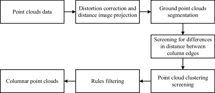

Block diagram of columnar point clouds extraction process
Road edges are another stable and common semantic feature structure in internal road environments in industrial parks. The extraction of road edge features means extracting the point clouds of point cloud line bundles as they cross the road edge. This type of point cloud located on the surface of the road boundary serves as a reference for the pavement area, which has the characteristics of continuity and stability, and is also able to improve the accuracy of map construction.
The point cloud located at the roadside will have some spatial characteristics different from the point cloud on the road surface:
-
(1)
For the point clouds on the road boundary surface on the same beam, the height difference between their neighbors in the vertical direction is significantly higher than that of their neighbors on the road surface, and the angle between the neighbors at the upper and lower boundaries of the road edge will change.
-
(2)
The point cloud on the road surface is vertically between the ground plane and the upper surface of the road.
The block diagram of roadside point clouds is shown in Fig. 2.


Block diagram of roadside point clouds extraction process
2.3 Feature Matching Associations for Fusion Semantics
The above implements the extraction of three types of point clouds: ground, columnar and roadside semantic features in a road environment with sparse features. These features can be repeatedly observed in two consecutive frames of the point cloud during the continuous motion of the LiDAR. Therefore, the position transformation obtained by correlation matching of the same category of feature point clouds in two consecutive frames is the position change of the carrier, and then the laser odometer is constructed through the consecutive position change.
For the matching and correlation of the same type of feature data, the point to line and point to surface correlation methods are usually used. The above three types of features extracted in this paper can be expressed as line and surface structures. Linear structure presents the characteristic of extending along a particular direction, while faceted structure unfolds in two directions. In this paper, from the characteristics of the feature point cloud itself, the three types of features are directly associated and matched in different ways; the columnar and roadside point clouds are matched and associated with the linear structure, while the ground point cloud is more suitable for the faceted structure.
For the columnar features, the point cloud presents a short bundle of multiple dense point clouds with parallel upward distribution in space. A point \({\text{p}}_{{\text{a}}}\) in the point cloud of the current frame is selected to find the nearest neighbor \({\text{p}}_{{\text{b}}}\) corresponding to the previous frame, and the nearest point of this nearest neighbor in the adjacent line bundles to construct the point-to-line data association. The coordinates of the point under the LiDAR coordinate system are denoted as follows, respectively. The point-to-line association matching equation is denoted as:
For roadside features, the distribution of the point cloud in space is a line structure stretching along the road, and the selection of the nearest points of the neighboring line bundles can reflect the line structure of the roadside, and the same point to line data association is taken through the above process.
For the ground feature point cloud, the point \(p_{i}\) of the current frame is selected with the nearest neighbour \(p_{j}\) corresponding to the previous frame, and the two nearest points \(p_{l}\) and \(p_{m}\) on the adjacent line bundle to construct the point-to-face data association. The coordinates of points \({\text{p}}_{{\text{i}}}\), \({\text{p}}_{{\text{j}}}\), \({\text{p}}_{{\text{l}}}\), \({\text{p}}_{{\text{m}}}\) under the LiDAR coordinate system are noted as: \({\text{X}}_{{\left({{\text{k,p}}_{{\text{i}}}} \right)}}^{{\text{L}}},{\text{X}}_{{\left({{\text{k - 1,p}}_{{\text{j}}}} \right)}}^{{\text{L}}},{\text{X}}_{{\left({{\text{k - 1,p}}_{{\text{l}}}} \right)}}^{{\text{L}}},{\text{X}}_{{\left({{\text{k - 1,p}}_{{\text{m}}}} \right)}}^{{\text{L}}}\). The point-to-face association matching equation is expressed as:
During the point-to-face data association process, the selection of similar feature points that are not co-linear can help to avoid the degradation of the plane composed of three points into a straight line. The above point-to-line and point-to-face data association is illustrated in Fig. 3, with the green line representing the previous frame point cloud and the dark brown line representing the current frame point cloud.


Fusion of semantic features for matching associations
The matching equations for the inter-frame features are obtained by the above process, and inter-frame six-degree-of-freedom bit-pose \(\left[{{\text{p}}_{{\text{x}}} {\text{,p}}_{{\text{y}}} {\text{,p}}_{{\text{z}}} {,\uptheta}_{{{\text{roll}}}} {,\uptheta}_{{{\text{pitch}}}} {,\uptheta}_{{{\text{yaw}}}}} \right]\) transform needs to be optimally solved. Remember that the bit-pose transform from frame \({\text{k}} - {1}\) to frame \({\text{k}}\) is \({\text{T}}_{{{\text{k}} - {1}}}^{{\text{k}}}\), then:
The line-plane association matching constraint equations with respect to \({\text{T}}_{{{\text{k}} - {1}}}^{{\text{k}}}\) are respectively:
Uniformly recorded as:
Each row in \({\text{f}}\) represents the feature point cloud and \({\text{d}}\) contains the corresponding distance relationship. The solution of the above equation is a nonlinear least squares optimisation problem. Firstly the Jacobi matrix \({\text{J}}\) of the matrix \({\text{f}}\) with respect to the variable \({\text{T}}_{{{\text{k}} - {1}}}^{{\text{k}}}\) is computed:
After obtaining the minimum value of d, the position can be optimized in two iterative steps with the help of the following equation:
where λ is the coefficient factor of the Levenberg–Marquardt method.
The two-step optimization to accelerate the solution of the \({\text{T}}_{{{\text{k}} - {1}}}^{{\text{k}}}\) transform is performed by the Levenberg–Marquardt method, where the IMU can provide the initial value of the bit-pose for the above solution, and the Levenberg–Marquardt method interpolates prior to the Gaussian Newton and gradient descent methods, which is a confidence domain method. Compared to the Gaussian Newton method, the Levenberg–Marquardt method is more robust and in most cases converges quickly and iteratively even if the unfolding point is very far from the final minimum. The flow of the LM two-step optimization algorithm is schematically shown in Fig. 4. \({\text{T}}_{{{\text{k}} - {1}}}^{{\text{k}}}\) contains six degrees of freedom poses, and for the ground feature points, the above three degrees of freedom poses are solved first by the first step of the LM algorithm because of better constraints on \(\left[{{\text{t}}_{{\text{z}}} {,\uptheta}_{{{\text{roll}}}} {,\uptheta}_{{{\text{pitch}}}}} \right]\). While reducing the number of optimisation iterations, the LM algorithm provides initial values for the constraint solving of \(\left[{{\text{t}}_{{\text{x}}} {\text{,t}}_{{\text{y}}} {,\uptheta}_{{{\text{yaw}}}}} \right]\) in the second step, thus speeding up the solving speed and finally obtaining a more accurate result of the position transformation [8, 9].


Schematic flow of the LM two-step optimization algorithm
2.4 Loop Closure Detection Based on Scan Context
The Scan Context (SC) [10] based method transforms the 3D point cloud into a 2D image with rotational invariance, i.e., column vector height invariance, according to the idea of dimensionality reduction. As this paper is oriented to the outdoor scene with sparse features, the road environment is mostly a turning road and there are more trees on both sides of the road, which have more stable ground plane features and rich columnar features, and the land on both sides of the road is uneven, with large feature variability in the height direction. Therefore, this paper introduces the Scan Context method in loop detection to improve the computational efficiency and ensure sufficient accuracy.
3 Sparse Feature Environment Mapping Experiment
The Lidar used is RS-LiDAR-16, set the rotational speed of 600 rpm, then the point cloud scanning frequency of 10 Hz. 9-axis IMU is used, model CH110, the angular velocity and acceleration output frequency of IMU is set to 100 Hz, and the internal parameter calibration of IMU is required before use, which is achieved by Allan variance is set to 100 Hz, the internal parameter calibration of the IMU needs to be carried out before use, which is achieved by Allan variance, and the IMU in this paper has been calibrated in advance. The software platform for the experiments of graph building algorithms is Ubuntu 18.04-Melodic operating system.
The scenario chosen for the test is a small field multi-loop scenario, which is a satellite image of a driving school’s subject 2 training field in Shanghai, which has a length of about 200 m in the horizontal direction and a width of about 60 m. The length of the experimental trajectory in Scenario 1 is about 900 m. It is found from the satellite image and the fieldwork that the test environment is characterized by both smooth planar features of the road as well as the road edge features on the two sides of the road, which This is conducive to the extraction of planar and semantic features.
The absolute trajectory error data for the ablation experiments for the small-field multi-loop scenario are shown in Table 1. Comparing the constructed trajectories without any semantic feature extraction, the absolute trajectory error is significantly larger than the result after extracting the semantic features in all indicators except the minimum value. When only column features or only roadside features are extracted, the average value of absolute trajectory error is about 0.21 m. When two types of semantic features are extracted at the same time, the average value of the absolute trajectory error is about 0.18 m, and the rest of the indicators except the minimum value are the smallest values in the same category.
Comparison of the map building effect shown in Fig. 5a is the map building effect of the A-LOAM algorithm, due to the poor processing of A-LOAM on the rotation of the mobile carrier, the point cloud map building in the feature part of the fence wall produces a large re-shadowing, as shown by the white box in Fig. 5a, and the mobile carrier at this time is in the rotational movement of the larger angular velocity, so that the construction of the point cloud map as a whole also produces a larger angle of the rotation error Therefore, the map constructed by A-LOAM also has a large rotational error, which ultimately leads to the failure of the map construction. In addition, A-LOAM does not differentiate between ground and non-ground feature points, so the quality of the map is not high.


Comparison of the effects of mapping
Figure 5b shows the local map building effect of this paper’s algorithm, and it can be clearly seen that the point cloud building effect of the fence part is better, with small ghosting and good consistency. In addition, thanks to the fusion of IMU and LiDAR, the map does not drift when the mobile carrier rotates at a large angular velocity, and the distinction between different features in the environment, such as roadside, tree trunks, foliage, fences, etc., is more obvious, and the quality of the map is higher.
As shown in Table 2 is the comparison of absolute trajectory error data for multiple loop scenarios in small sites. The absolute trajectory errors built by the algorithm of this paper have been improved in terms of mean and median. Comparing with LeGO algorithm, it can be clearly seen that this paper can effectively reduce the trajectory error and improve the accuracy of map building by extracting semantic features.
Combined with Table 3, the relative trajectory error of this paper’s algorithm in the small field multi-loop scenario performs better in terms of the maximum value than with the LeGO algorithm, and the rest is basically the same. This is mainly due to the fact that the environment of the small field multi-loop scenario has only sparse features such as trees, road edges, and land to construct the odometer, so the variation of the error does not vary greatly.
As shown in Table 4 is a comparison of the different number of loop closure detections obtained and the absolute trajectory error of each data before and after the loop closure detection strategy is adopted. Before adopting the loop closure detection strategy, 106 loop closure detections were successfully detected and loop closure detection constraints were constructed. After adopting the loop closure detection strategy, 80 loop closure detections were successfully detected, and the number of loop closure detections were significantly reduced, which saves the resource overhead. In the end, the reduction in the number of loopback detections is about 28% with a slight reduction in the accuracy of the build trajectory and a small impact, reducing the number of ineffective and frequent loop closure detections by a certain amount.
4 Conclusion
This paper presents research and experiments on mapping algorithms for road scenes with sparse features. The experimental scenario, i.e., a road scene with multiple loops in a small field, is introduced. Evaluation metrics are employed to analyze the mapping trajectory. Ablation experiments are conducted to validate the effectiveness of semantic features. Mapping experiments are performed in this scenario to assess the performance of the proposed algorithm, and comparisons with other algorithms demonstrate its superiority in improving mapping trajectory accuracy. Additional experiments verify the effectiveness of the loop closure strategy, which reduces the number of invalid detections without compromising accuracy. However, the robustness of LiDAR mapping algorithms is low in weak geometry environments, and fusion of more sensors, such as LiDAR-camera fusion for mapping tasks, can be considered in the future.
References
Badue CF (2021) Self-driving cars: a survey. Expert Syst Appl 165:113816
Lu YF (2021) Real-time performance-focused on localization techniques for autonomous vehicle: a review. IEEE Trans Intell Transp Syst 23(7):6082–6100
Sandström EF (2023) Point-slam: dense neural point cloud-based slam. In: Proceedings of the IEEE/CVF international conference on computer vision. IEEE, Paris, pp 18387–18389
Liso LF (2024) Loopy-slam: dense neural slam with loop closures. In: Proceedings of the IEEE/CVF conference on computer vision and pattern recognition. IEEE, Seattle, pp 20363–20373
Wang HF (2023) Co-slam: joint coordinate and sparse parametric encodings for neural real-time slam. In: Proceedings of the IEEE/CVF conference on computer vision and pattern recognition. IEEE, Vancouver, pp 13293–13302
Wang ZF (2021) Pole-like objects mapping and long-term robot localization in dynamic urban scenarios. In: International conference on robotics and biomimetic. IEEE, Sanya, pp 998–1003
Chiang KWF (2020) Performance enhancement of INS/GNSS/refreshed-SLAM integration for acceptable lane-level navigation accuracy. IEEE Trans Veh Technol 69(3):2463–2476
Ran HF (2022) Surface representation for point clouds. In: Proceedings of the IEEE/CVF conference on computer vision and pattern recognition. IEEE, New Orleans, pp 18942–18952
Boulch AF (2022) Poco: Point convolution for surface reconstruction. In: Proceedings of the IEEE/CVF conference on computer vision and pattern recognition. IEEE, New Orleans, pp 6302–6314
Kim GF (2018) Scan context: egocentric spatial descriptor for place recognition within 3d point cloud map. In: 2018 IEEE/RSJ International Conference on Intelligent Robots and Systems (IROS). IEEE, Madrid, pp 4802–4809
Acknowledgements
Supported by the National Key Research and Development Program of China (Grant No. 2023YFF0613200).
Author information
Authors and Affiliations
Corresponding author
Editor information
Editors and Affiliations
Rights and permissions
Open Access This chapter is licensed under the terms of the Creative Commons Attribution-NonCommercial-NoDerivatives 4.0 International License (http://creativecommons.org/licenses/by-nc-nd/4.0/), which permits any noncommercial use, sharing, distribution and reproduction in any medium or format, as long as you give appropriate credit to the original author(s) and the source, provide a link to the Creative Commons license and indicate if you modified the licensed material. You do not have permission under this license to share adapted material derived from this chapter or parts of it.
The images or other third party material in this chapter are included in the chapter’s Creative Commons license, unless indicated otherwise in a credit line to the material. If material is not included in the chapter’s Creative Commons license and your intended use is not permitted by statutory regulation or exceeds the permitted use, you will need to obtain permission directly from the copyright holder.
Copyright information
© 2026 The Author(s)
About this paper

Cite this paper
Ding, Z., Li, T., Xie, L., Bian, Y. (2026). Sparse Feature-Oriented 3D SLAM Mapping with Semantic Fusion. In: Saman, H., Peng, Y., Zhao, D., Bian, Y. (eds) The 9th International Conference on Advances in Construction Machinery and Vehicle Engineering. ICACMVE 2024. Lecture Notes in Mechanical Engineering. Springer, Singapore. https://doi.org/10.1007/978-981-96-5527-4_52
Download citation
DOI: https://doi.org/10.1007/978-981-96-5527-4_52
Published:
Publisher Name: Springer, Singapore
Print ISBN: 978-981-96-5529-8
Online ISBN: 978-981-96-5527-4
eBook Packages: Mechanical Engineering (R0)Springer Nature Proceedings excluding Computer Science