Isothermal Attachment Ventilation Mechanisms

Abstract

This chapter expounds on the airflow mechanisms of isothermal vertical wall attachment ventilation, rectangular column attachment ventilation, and circular column attachment ventilation. This chapter presents the characteristic parameters of the isothermal attachment ventilation and the airflow characteristics in the vertical attachment, jet impingement, and horizontal air reservoir regions. The parameter correlations of velocity distribution (maximum velocity or centerline velocity decay and cross-sectional velocity profiles), jet thickness, cross-sectional airflow rate of attachment ventilation, etc., have been established.

This chapter elaborates on the air distribution mechanisms of isothermal attachment turbulent jets, mainly including the air velocity distributions in the vertical attachment and horizontal air reservoir regions. There is a significant difference between the motion characteristics of the wall-attached jet and the free jet. This chapter presents the characteristic parameters of the isothermal wall-attached jet and the airflow movement feature in the vertical attachment, jet impinging, and horizontal air reservoir regions for VWAV and CAV. The interaction between the wall-attached jet and the vertical wall and floor is determined (region I–III). The parameter correlations of velocity distribution (maximum velocity or centerline velocity decay and cross-sectional velocity profiles), jet thickness, cross-sectional airflow rate of attachment ventilation, etc., have been established.

In solving the problems of design ventilation, it is necessary to take the following factors into account:

• 1. airflow rate supplied to and extracted from the room;

• 2. characteristic parameters of the incoming air and the treatment of the air, including heating, cooling, etc.;

• 3. layout and geometric parameters of the inlets and outlets;

• 4. geometric shape and size of the room;

• 5. location and capacity of sources that change air composition and state, in particular, sources of heat and pollution;

• 6. air currents created by these sources, human behaviors, and industrial production activities.

3.1 Wall-Attached Jet Parameters

When the air supply opening is located in the upper part of the vertical wall (or its vicinity, not exceeding the maximum attachment distance), the supply air jet forms a confined wall-attached jet caused by the Coanda effect and extended Coanda effect (Li 2019). Generally, this wall jet can be divided into a boundary layer closing to the wall surface and a free-shear flow away from the wall.

The turbulent wall-attached jet can also be divided into inner and outer layers. In the inner layer (near the wall surface), the flow field is similar to that of the flat plate or plane boundary layer; in the outer region, the flow field is similar to that of a free jet. The inner layer and outer region are bounded by u = u_m, as shown in Fig. 3.1.

Fig. 3.1

Inner and outer layers of a turbulent wall-attached jet (bounded by u = u_m)

From the perspective of ventilation and air-conditioning, the whole room can be divided into a jet-dominating zone (including an inner layer and outer layer) and an air-diffusing zone (u ≤ 0.3 m/s for environment allowable velocity, which can be extended to 0.8 m/s for the temporary staying zone, such as subway stations, industrial plants, occupied zone of hydropower plants). ASHRAE 55-2017 specifies that the maximum acceptable velocity is 0.8 m/s when the operating temperature is 26 °C.

Concerning the wall-attached jet parameters, the fundamental characteristic parameters are assumed as follows. For wall-attached jets entering a steady-state environment, the fundamental parameters are centerline velocity u_m (i.e., maximum velocity), jet thickness, the width of slot b, and velocity at the slot inlet u₀. The inner layer thickness δ_m is the normal distance between the wall and the point where the attached jet velocity is equal to u_m; characteristic thickness δ_0.5 is the normal distance between the wall and the point where the attached jet velocity is equal to 0.5u_m in the outer layer of the wall-attached jet; total thickness δ₀ is the normal distance between the wall and the outer layer boundary, as illustrated in Fig. 3.2a. These parameters of the wall-attached jet can be normalized as dimensionless characteristic parameters. The wall-attached jet features are mainly related to the supply air velocity (u₀), supply and exhaust air temperature (t₀, t_e), indoor load (Q), and supply and exhaust opening positions (h, S), etc. For a jet attached to a smooth wall, the dimensionless characteristic parameters mainly include:

Fig. 3.2

a Theoretical analysis of the wall-attached jet, b coordinate system used for wall-attached jets analysis. Note The centerline velocity in this book is defined as the maximum velocity of the jet

• Centerline velocity of the wall-attached jet $\frac{{u_{\text{m}} }}{u_0 }$;

• Velocity profile of the jet main section $\frac{u}{{u_{\text{m}} }}$;

• Characteristic thickness of the jet $\delta_{0.5}$;

• Cross-section airflow rate along the jet direction $\frac{Q}{Q_0 }$;

• The dimensionless excess temperature of the jet centerline $\frac{{t_{\text{m}} - t_{\text{n}} }}{{t_0 - t_{\text{n}} }}$ (for a nonisothermal jet).

In addition, for deflected wall-attached jets, the position of the attachment point (see Fig. 3.2a) should also be taken into account.

The parameters characterizing the jet’s fundamental features are jet centerline velocity u_m(x, y), section thickness δ(x, y), and cross-sectional velocity u(x, y).

For the sake of discussion, the origin of the coordinate system used in this book is located at the intersection of the jet-attached wall surface and the floor, as shown in Fig. 3.2a.

It should be noted that for flow-field analysis of the wall-attached jet, two Cartesian coordinate systems are adopted, namely x–y and x–y^*. The z-axis is perpendicular to the coordinate plane, as shown in Fig. 3.2b. The difference between these two coordinate systems lies in that y and y^* are in opposite directions, i.e., y^* = h – y, where h is the slot’s installation height. In this book, the x–y^* coordinate system is mainly used in the theoretical analysis of the wall-attached jet (see Fig. 3.2b).

The characteristic parameters of the wall-attached jet are shown in Table 3.1.

Table 3.1 Dimensionless characteristic parameters of the wall-attached jet

3.2 Jet Impinging Region

The jet impinging region is defined as the region where the jet velocity and pressure, etc., are affected by impinging within the scope of HVAC. This region is usually 0.5–1.0 m away from the vertical wall and horizontal floor, respectively (see Fig. 3.2a). In the jet impinging region, it can be found that the adverse pressure gradient increases as the jet approaches the floor. As illustrated in Fig. 3.3a, it can be observed there are the vortical structures in the jet impinging region, where a large-scale vortex is generated, and secondary vortexes at the corner are induced. The direction of vortex recirculation is approximately opposite to that of mainstream movement. The separation point and reattachment point could characterize the location of the large-scale vortex in the jet impinging region. The separation point $(\partial u_y /\left. {\partial x} \right|_{x = 0} = 0)$ is located at the end of the vertical attachment region, which is also treated as the start of the jet impinging region. Likewise, the reattachment point $(\partial u_x /\left. {\partial y} \right|_{y = 0} = 0)$ lies at the end of the jet impinging region and the start of the horizontal air reservoir region. The separation point and reattachment point are expounded in more detail as follows.

Fig. 3.3

a Velocity-vector field with streamlines in the jet impinging region, b reattachment point location, c separation point h_s/b as a function of (h/b)^2/3Re^−1/3, d reattachment point l_a/b as a function of (h/b)^2/3Re^−1/3

For an isothermal wall-attached jet, it can be expressed in a dimensionless form based on experimental and numerical results. In the range of 0.5 ≤ (h/b)^2/3Re^−1/3 ≤ 1.2 (see Fig. 3.3c), the separation point can be determined by the Eq. (3.1a)

$$\frac{h_s }{b} = 11.8\left( \frac{h}{b} \right)^\frac{2}{3} {\text{Re}}^{ - \frac{1}{3}}$$

(3.1a)

where h_s is the normal distance between the floor and the separation point, see Fig. 3.3a. It could be regarded as a function of jet discharge velocity u₀, opening height h, opening width b, air density ρ, and air kinetic viscosity μ, etc.

Similarly, the reattachment point (see Fig. 3.3b, d) is presented by Eq. (3.1b)

$$\frac{{l_{\text{a}} }}{b} = 7.9\left( \frac{h}{b} \right)^\frac{2}{3} {\text{Re}}^{ - \frac{1}{3}}$$

(3.1b)

where l_a is the normal distance between the attached wall and the reattachment point, see Fig. 3.3a, b. In the range discussed above, it can be concluded that $\frac{{l_{\text{a}} }}{h_s } \approx 0.67$.

Figure 3.4 shows the velocity contours corresponding to different air supply velocities in the jet impinging and horizontal air reservoir regions. With the enhancement of u₀, from 1.0 m/s to 2.0 m/s, it can be observed that the clockwise vortex in the corner diminishes. For the increment of velocity, the jet impinging on the floor is further enhanced, and the air around the corner gets more squeezed, which narrowly the circumfluence vortex correspondingly. The comparison results of the corner regions of Fig. 3.4a, c, d, f further support this argument. These findings provide insights into the role of the wall-attached jet impinging region.

Fig. 3.4

Indoor air velocity distributions with different air supply velocities, a–f airflow patterns of the impinging region or corner, g dimensionless centerline velocity of the horizontal region as a function of distance x/b

It can be obtained from Fig. 3.4g, that the jet centerline velocity profile shows similarity in the horizontal region (region III), except the jet impinging region (region II). In region II, the air “initial velocity” (maximum centerline velocity in region II) grows with the supply air velocity increasing (dynamic pressure regaining). For a given velocity u₀ = 1.5 m/s, 3.0 m/s and 5.0 m/s, the “initial velocity” reaches 0.6 m/s, 1.3 m/s and 2.25 m/s, respectively. It is also observed that the centerline velocity in the jet impinging region is approximately symmetrical along the bisector of 90°.

The angle between two adjacent walls also influences the flow field. When the jet opening is located in a room’s intersection area (concave corner), the jet’s boundary changes significantly with the air velocity. Figure 3.5 demonstrates the forms of the boundary layer at the angle area of 60° between two walls (dihedral angle). If expressed in polar coordinates, it can be seen that there is an interface point between laminar flow and turbulent flow at the angular bisector to the apex of the angle (Sun 1992). The wall-attached jet flow is related to the angle’s sharpness degree and Reynolds number Re (i.e., velocity) of supply air. When Re increases, the laminar flow area in the angle area will become smaller (Sun 1992). The sharper angle is in response to the larger viscous sublayer.

Fig. 3.5

Boundary layer of the concave corner (Sun 1992)

3.3 Isothermal Vertical Wall Attachment Ventilation Parameter Correlations

The air movement of a ventilated room depends on the time-averaged flow and turbulence characteristics of the air jet and thermal plume. Air distribution in ventilated spaces only the steady-state flow situation is considered. To achieve a well-designed room air distribution, it is necessary to understand the mechanisms and prediction method of airflow. This section presents mathematical models and semi-empirical expressions for predicting wall-attached jet flow.

Generally, the velocity components of a turbulent wall-attached jet can be decomposed into a time-averaged u_m and fluctuating components $u^{\prime}$, $v^{\prime}$, $w^{\prime}$. Eckert once investigated the fluctuating velocity components $u^{\prime}$, $v^{\prime}$, $w^{\prime}$ in the jet boundary layer of the smooth wall. Results indicate that the fluctuating velocities $u^{\prime}$, $v^{\prime}$, $w^{\prime}$ are about 4–8% of the time-averaged velocity u_m for the wall-attached jet boundary layer in the mainstream (see Fig. 3.6) (Eckert and Drake 1972). Hence, the time-averaged velocity distributions, in the vertical attachment region and the horizontal air reservoir region have proved to be satisfactory in reflecting the fundamental features of the attachment ventilation.

Fig. 3.6

Fluctuating velocity components in the boundary layer of a wall jet (Eckert and Drake 1972)

This section presents the time-averaged velocity distribution and corresponding expressions or correlations under isothermal conditions in detail.

3.3.1 Centerline Velocity in Vertical Attachment Region

So far, the theoretical calculation of the turbulent boundary layer of the incompressible flow has not developed enough to get rid of the semi-empirical theory. In this book, the author attempts to establish semi-empirical theoretical expressions of the centerline velocity distributions of attachment ventilation. For the wall-attached jet, the following conclusions can be obtained from the visualization investigation in the previous chapters:

• 1. In the fully developed region, there is a similarity of the time-averaged velocity distributions (e.g., centerline velocity and cross-sectional velocity) of the wall-attached jet, which can be described by $f(\frac{u}{u_0 },\frac{y^* }{b},\frac{x}{b}) = 0$ (see Fig. 3.2b).

• 2. For the centerline velocity of the two-dimensional wall-attached jet, the function can be simplified as $f(\frac{{u_{\text{m}} }}{u_0 },\frac{y^* }{b}) = 0$ and $f(\frac{{u_{\text{m}} }}{u_0 },\frac{x}{b}) = 0$ in the vertical attachment region and horizontal air reservoir region, respectively.

The centerline velocity’s semi-empirical expression has been derived theoretically and experimentally, using the hypothesis for free turbulent flow due to Prandtl (1942). The air movement in the wall-attached jet is a self-similar flow with a universal flow profile. That is to say, for different distances y^*, the velocity profiles derived is shown to be identical as long as the scale factors of velocity and width are appropriately selected.

The equations governing a turbulent wall-attached jet are considered here. On the boundary layer approximation, the pressure is uniform everywhere, and the eddy viscosity $\in$ is introduced. The momentum and continuity equations are given by Eqs. (3.2a) and (3.2b), respectively

$$u\frac{\partial u}{{\partial y^* }} + v\frac{\partial u}{{\partial x}} = \frac{\partial }{\partial x}\left( { \in \frac{\partial u}{{\partial x}}} \right)$$

(3.2a)

$$\frac{\partial u}{{\partial y^* }} + \frac{\partial v}{{\partial x}} = 0$$

(3.2b)

The boundary conditions are

$$\begin{aligned} & u = v = 0\;{\text{at}}\;x = 0; \\ & u \to 0\;{\text{as}}\;x \to \infty \left( {{\text{ambient}}\;{\text{fluid}}\;{\text{velocity}}\;{\text{is}}\;0} \right) \\ \end{aligned}$$

where

y ^* :

distance along the wall measured from the slot opening, m;

x :

distance normal to the wall, m;

u :

velocity component along the y^* direction, m/s;

v :

velocity component along the x-direction, m/s;

∈:

eddy viscosity.

Assumptions regarding the eddy viscosity ∈ are made according to Prandtl’s hypothesis for free turbulent flow (Prandtl 1942). The eddy viscosity is constant across the breadth of the jet, and is proportional to the product of the maximum difference between time-averaged velocity and width of the layer

$$\in = \rho k\delta (\overline{u}_{\max } - \overline{u}_{\min } )$$

where

ρ :

density, kg/m³;

k :

a universal constant;

δ :

a typical measure of the boundary layer width, m;

$\overline{u}_{\max } - \overline{u}_{\min }$ :

the maximum difference of the time-average velocity in the fluid micro-cluster, m/s. It is obtained from a lot of measured data of free turbulent jets by Prandtl.

Consider the possibility that there shall be a similarity solution of Eq. (3.2a) (Glauert 1956)

$$\begin{aligned} & u \sim y^{*{\text{p}}} ,\delta \sim y^{*{\text{q}}} , \in \sim y^{*\rm{p} + {\text{q}}} \\ & \frac{\partial u}{{\partial y^\ast }} \sim p - 1,u\frac{\partial u}{{\partial y^\ast }} \sim 2p - 1 \\ \end{aligned}$$

According to the boundary layer theory, x is the distance normal to the wall and thus has the same magnitude with δ, i.e., $x \sim \delta$, we obtain

$$\frac{\partial }{\partial x}\left( { \in \frac{\partial u}{{\partial x}}} \right) \sim 2p - q$$

The two sides of Eq. (3.2a) should vary with y in the same manner, thus

$${2}p - {1} = {2}p - q,q = {1}$$

(3.3)

Introduce (external) momentum flux F below. Multiply Eq. (3.2a) by y^* and integrate with respect to x between the limits x and ∞, we have

$$\int\limits_x^\infty {y^* u\frac{\partial u}{{\partial y^* }}{\text{d}}x} + \int\limits_x^\infty {y^* v\frac{\partial u}{{\partial y^* }}{\text{d}}x} = \int\limits_x^\infty {y^* \in \frac{\partial^2 u}{{\partial x^2 }}{\text{d}}x}$$

(3.4)

Considering u → 0 as x → ∞, Eq. (3.4) is simplified as

$$\frac{\partial }{\partial y^* }\int\limits_x^\infty {y^* u^2 {\text{d}}x} - y^* vu + y^* \in \frac{\partial u}{{\partial x}} = 0$$

(3.5)

Multiplying by y^*u, and integrating with respect to x between the limits 0 and ∞, we then have

$$\begin{aligned} & \frac{\partial }{\partial y^* }\int\limits_x^\infty {y^* u\left\{ {\int\limits_x^\infty {y^* } u^2 {\text{d}}x} \right\}{\text{d}}x} - \int\limits_x^\infty {\frac{\partial (y^* u)}{{\partial y^* }}\left\{ {\int\limits_x^\infty {y^* } u^2 {\text{d}}x} \right\}{\text{d}}x} \\ & \quad - \int\limits_0^\infty {y^{*2} vu^2 {\text{d}}x + \left[ {\frac{1}{2} \in y^{*2} u^2 } \right]_0^\infty = 0} \\ \end{aligned}$$

(3.6)

From the continuity equation, the second term of Eq. (3.6) is

$$- \left[ {y^* v\int\limits_x^\infty {y^* u^2 {\text{d}}x} } \right]_0^\infty + \int\limits_0^\infty {y^{*2} vu^2 {\text{d}}x}$$

At x = 0, u = v = 0; at x → ∞, u → 0, so Eq. (3.6) reduces to

$$\frac{\partial }{\partial y^* }\int\limits_0^\infty {y^* u} \left\{ {\int\limits_x^\infty {y^* u^2 {\text{d}}x} } \right\}{\text{d}}x = 0$$

or

$$F = \int\limits_0^\infty {y^* u} \left\{ {\int\limits_x^\infty {y^* u^2 {\text{d}}x} } \right\}{\text{d}}x = {\text{constant}}$$

(3.7)

The physical significance of Eq. (3.7) is that the external momentum flux is conserved. In the case of a similarity solution, $x^2 \sim \delta^2 \sim y^{*2{\text{q}}}$, and $u \sim y^{*{\text{p}}}$, so Eq. (3.7) shows that

$${3}p + {2}q + {2} = 0$$

(3.8)

Equations (3.3) and (3.8) now show that,

$$p = - \frac{4}{3},q = 1$$

(3.9)

Thus

$$u \sim (y^* )^{ - \frac{4}{3}} ,\delta \sim (y^* )^1$$

If

$$\frac{u}{{u_{\text{m}} }}{\text{ = g}}\left( {\frac{x}{\delta }} \right)$$

(3.10)

Considering the dimensional consistency, we have

$$u_{\text{m}} \sim (y^* )^{ - \frac{4}{3}}$$

Therefore, the centerline velocity u_m of the wall-attached jets is represented by

$$\frac{{u_{\text{m}} \left( {y^* } \right)}}{u_0 } \sim \left( {\frac{y^* }{b}} \right)^{ - \, \frac{{4}}{{3}}}$$

(3.11a)

or

$$\frac{u_0 }{{u_{\text{m}} \left( {y^* } \right)}} \sim \left( {\frac{y^* }{b}} \right)^\frac{4}{3}$$

(3.11b)

Equation (3.11a, 3.11b) is derived based on Prandtl’s hypothesis, i.e., the eddy viscosity is constant across the breadth of the jet, which is drawn from measured data of free turbulent jets. Therefore, it is understandable that there shall be some differences when the expression is used for the wall-attached jet. It can be assumed that the centerline velocity of the wall-attached jet in the vertical attachment region (main region) has a negative γ power function relation with y^*, which is expressed as Eq. (3.12)

$$\frac{u_0 }{{u_{\text{m}} \left( {y^* } \right)}} \sim \left( {\frac{y^* }{b}} \right)^\frac{4}{3} ,\quad \gamma > 0$$

(3.12)

where γ is determined by experimental data, which indicates the momentum decay rate of the wall-attached jets.

Figure 3.7 shows the characteristic parameters and the centerline velocity decay in the vertical attachment region for vertical wall attachment ventilation. The parameters are shown in Fig. 3.7a, and Fig. 3.7b presents centerline velocity decay under different slot heights h, and air supply velocities u₀ in the vertical attachment region. The centerline velocity decay shown in Fig. 3.7b agrees well with the above theoretical analysis.

Fig. 3.7

Semi-empirical correlation of centerline velocity in the vertical attachment region and compared with a free jet. a Characteristic parameters, b centerline velocity distribution in the vertical attachment region

Based on the theoretical analysis and experimental data of attachment ventilation, the semi-empirical correlations Eq. (3.13) of the centerline velocity decay in the vertical attachment region is proposed for engineering applications.

$$\frac{{u_{\text{m}} \left( {y^* } \right)}}{u_0 } = \frac{1}{{0.01\left( {\frac{y^* }{b}} \right)^{1.11} + 1}}$$

(3.13)

It can be seen that the factors affecting the centerline velocity distribution are as follows: air supply velocity u₀, vertical distance along the vertical wall measured from the slot opening y^* (y^* = h − y, reflecting the effect of room height h), characteristic dimension b of the slot, and exhaust outlet (the exhaust outlet is also called as the air inlet in ANSI/ASHRAE Standard 113 (2013) and ASHRAE Handbook: Fundamentals (2017)) forms, etc. As illustrated in Fig. 3.7, the centerline velocity decay shows similarity in the vertical attachment region with different air supply heights h and air supply velocities u₀. In the range of 0 ≤ y^*/b ≤ 40, the centerline velocity of the jet decays rapidly (a large curve slope). When the jet continues to move downward along the vertical wall, the centerline velocity declines slowly till it reaches the separation point, $\partial u_y {/}\partial x\mid_{x = 0} = 0$, where the jet turns out to be separated from the vertical wall.

The free jet’s centerline velocity decay is simultaneously shown in Fig. 3.7. It can be observed that the curve slope of the wall-attached jet is much less than that of the free jet. That is to say, the centerline velocity of the vertical wall-attached jet decays more slowly. For the same discharge velocity, it means that the wall-attached jet can reach a much further distance. For instance, at y^*/b = 40, the centerline velocity of the free jet is only approximately 20% of the wall-attached jet.

3.3.2 Centerline Velocity in Horizontal Air Reservoir Region

As mentioned above, when separating from the vertical wall, the wall-attached jet impinges on the floor, then expands in a radial pattern and moves along the floor, forming an air reservoir at the horizontal floor. The air reservoir is directly related to the conditioned environment of the occupied zone, so it is vital to establish the centerline velocity distributions in the horizontal air reservoir region. Figure 3.8 illustrates the dimensionless centerline velocity decay in the horizontal air reservoir region. Likewise, it can be drawn that the dimensionless centerline velocity demonstrates similarity. The decay rate of the centerline velocity is relatively lower in the horizontal air reservoir region than in the vertical attachment region.

Fig. 3.8

Characteristic parameters and centerline velocity decay in the horizontal air reservoir region (S/b = 0). a Characteristic parameters, b centerline velocity decay in the horizontal air reservoir region

According to the dimensional analysis, the centerline velocity u_m in the horizontal air reservoir region is primarily related to the air inlet types, the air supply velocity u₀, the distance normal to the wall x, the characteristic dimension b of the inlet, and the air supply height h, which can be expressed as

$$f\left( {\frac{{u_{\text{m}} \left( x \right)}}{u_0 },\frac{x}{b},\frac{h}{b}} \right) = 0$$

(3.14)

Figure 3.8b represents plots of dimensionless centerline velocity u_m(x)/u₀ versus dimensionless distance $x/b + {K_{\text{h}}}$ in the horizontal air reservoir region. It can be observed that the dimensionless curve of centerline velocity decay is identical for different air supply heights h and air supply velocities u₀. Although the centerline velocity is different for different positions of the horizontal air reservoir region, centerline velocity similarity still exists in this region.

Similarly, in the horizontal air reservoir region (see Fig. 3.8b), the centerline velocity of the wall-attached jet has negative α and β power function relations with the distance from the vertical wall x and the slot installation height h, respectively.

According to the experimental results, we have

$$\begin{aligned} & \frac{{u_{\text{m}} \left( x \right)}}{u_0 } \sim \left( \frac{x}{b} \right)^{ - \alpha } ,\frac{{u_{\text{m}} \left( x \right)}}{u_0 } \sim \left( \frac{h}{b} \right)^{ - \beta } \\ & \frac{{u_{\text{m}} \left( x \right)}}{u_0 } = \frac{0.575}{{0.0075\left( {\frac{x}{b} + K_{\text{h}}} \right)^{1.11} + 1}} \\ \end{aligned}$$

(3.15)

where

h :

air supply height, m,

$K_{\text{h}}$ :

correction factor, $K{_\text{h} = }\frac{1}{2}\frac{h - 2.5}{b}$. A reference height of 2.5 m for ordinary offices is adopted according to the Chinese standard JGJ67-2006 “Code for Design of Office Buildings”.

3.3.3 Cross-Sectional Velocity Profile

The flow of the wall-attached jet’s inner layer can be simplified according to the boundary layer theory. The governing equations are

$$\frac{\partial u}{{\partial y^{*} }} + \frac{\partial v}{{\partial x}} = 0$$

(3.16)

$$u\frac{\partial u}{{\partial y^{*} }} + v\frac{\partial u}{{\partial x}} = - \frac{1}{\rho }\frac{\partial p}{{\partial y^* }} + v\frac{\partial^2 u}{{\partial x^2 }} + \frac{1}{\rho }\frac{{\partial \tau_{\text{t}} }}{\partial x}$$

(3.17)

where $\tau_{\text{t}}$ denotes turbulent shear stress.

The self-similarity exists for the wall-attached jet on the smooth wall surface. $u_{\text{m}}$ is adopted as characteristic velocity, and the distance between the wall and the point where u = 0.5u_m in the outer layer of the wall-attached jet is regarded as characteristic thickness $\delta_{0.5}$ (for the sake of discussion, it may be expressed as δ). The cross-sectional velocity profile can be expressed as Eq. (3.18) (Zhang 2011)

$$\frac{u}{{u_{\text{m}} }} = f\left( {\frac{x}{\delta }} \right) = f\left( \eta \right)$$

(3.18)

If we write $\frac{{\tau_{\text{t}} }}{{\rho u_{\text{m}}^2 }} = g\left( \eta \right)$, and let $u_{\text{m}} \propto y^{*{\text{p}}}$, $\delta \propto y^{*{\text{q}}}$, the values of the exponents p, q can be obtained from the governing equations and similarity relation.

According to $u = u_{\text{m}} f\left( \eta \right)$ in Eq. (3.18), we obtain

$$\begin{aligned} & \frac{\partial u}{{\partial y^* }} = \frac{\partial }{\partial y^* }\left( {u_{\text{m}} f} \right) = u_{\text{m}} \frac{{{\text{d}}f}}{{{\text{d}}\eta }}\frac{\partial \eta }{{\partial \delta }}\frac{{{\text{d}}\delta }}{{{\text{d}}y^* }} \\ & \quad + f\frac{{{\text{d}}u_{\text{m}} }}{{{\text{d}}y^* }} = - u_{\text{m}} f^{\prime}\frac{x}{\delta^2 }\delta^{\prime} + fu^{\prime}_{\text{m}} \\ \end{aligned}$$

(3.19)

$$u\frac{\partial u}{{\partial y^{*} }} = u_{\text{m}} u^{\prime}_{\text{m}} f^2 - \frac{{u_{\text{m}}^2 \delta^{\prime}}}{\delta }\eta ff^{\prime}$$

(3.20)

According to Eq. (3.16), we have

$$\begin{aligned} & v = \int\limits_0^x {\frac{\partial v}{{\partial x}}{\text{d}}x} = - \int\limits_0^x {\frac{\partial u}{{\partial y}}{\text{d}}x} = \int\limits_0^x {\left( {\frac{{u_{\text{m}} \delta^{\prime}}}{\delta }\eta f^{\prime} - u^{\prime}_{\text{m}} f} \right){\text{d}}x} \\ & = u_{\text{m}} \delta^{\prime}\int\limits_0^x {\eta f^{\prime}{\text{d}}\eta - u^{\prime}_{\text{m}} \delta } \int\limits_0^x {f{\text{d}}x} \end{aligned}$$

(3.21)

$$\frac{\partial u}{{\partial x}} = \frac{\partial }{\partial x}\left( {u_{\text{m}} f} \right) = u_{\text{m}} f^{\prime}\frac{\partial \eta }{{\partial x}} = \frac{{u_{\text{m}} }}{\delta }f^{\prime}$$

(3.22)

$$v\frac{\partial u}{{\partial x}} = \frac{{u_{\text{m}}^2 \delta^{\prime}}}{\delta }f^{\prime}\int\limits_0^\eta {\eta f^{\prime}{\text{ d}}\eta - u_{\text{m}} u^{\prime}_{\text{m}} f^{\prime}} \int\limits_0^\eta {f{\text{d}}\eta }$$

(3.23)

$$\frac{1}{\rho }\frac{\partial \tau_t }{{\partial x}} = \frac{1}{\rho }\frac{\partial }{\partial x}\left( {\rho u_{\text{m}}^2 g} \right) = \frac{{u_{\text{m}}^{2} }}{\delta }\frac{\partial g}{{\partial \eta }} = \frac{{u_{\text{m}}^2 }}{\delta }g^{\prime}$$

(3.24)

where $\delta^{\prime} = \frac{{{\text{d}}\delta }}{{{\text{d}}y}}$, $u^{\prime}_{\text{m}} = \frac{{{\text{d}}u_{\text{m}} }}{{{\text{d}}y}}$, $f^{\prime} = \frac{{{\text{d}}f}}{{{\text{d}}\eta }}$, $g^{\prime} = \frac{{{\text{d}}g}}{{{\text{d}}\eta }}$

In most cases, the Reynolds number $\frac{{u_{\text{m}} \delta }}{v}$ is large, thus the viscosity term in Eq. (3.17) can be ignored. Considering $\frac{\partial p}{{\partial y^{*} }} = 0$, Eqs. (3.20), (3.23) and (3.24) now show that

$$g^{\prime} = \frac{{\delta u^{\prime}_{\text{m}} }}{{u_{\text{m}} }}\left( {f^2 - f^{\prime}\int\limits_0^\eta {f{\text{d}}\eta } } \right) - \delta^{\prime}\left( {\eta ff^{\prime} - f^{\prime}\int\limits_0^\eta {\eta f^{\prime}{\text{d}}\eta } } \right)$$

(3.25)

Since $g^{\prime}$ is a function of η only, the right side of Eq. (3.25) should also be a function of η, then $\frac{{\delta u^{\prime}_{\text{m}} }}{{u_{\text{m}} }}$ and $\delta^{\prime}$ should be independent of y, thus

$$\frac{{\delta u^{\prime}_{\text{m}} }}{{u_{\text{m}} }} \sim y^0 ,\delta^{\prime} \sim y^0$$

Thus q = 1, i.e., $\delta \sim y$.

According to the conservation of momentum, we have

$$\frac{{\text{d}}}{{{\text{d}}y}}\int\limits_0^\infty {\rho u^2 {\text{d}}x = 0}$$

(3.26)

Equations (3.18) and (3.26) show that

$$\frac{{\text{d}}}{{{\text{d}}y}}\rho u_{\text{m}}^2 \int\limits_0^\infty {f^2 {\text{d}}\eta = 0}$$

(3.27)

and hence $u_{\text{m}}^2 \delta \sim y^0$, 2p + q = 0.

Since q = 1, the we have p = − 0.5. Thus, $\delta_{_{0.5} } \sim y^*$, $\frac{{u_{\text{m}} }}{u_0 } \sim 1/\sqrt {\frac{y^* }{b}}$.

For the turbulent wall-attached jet, the cross-sectional velocity profile obtained from experiments agrees well with the results from Glauert (1956), Verhoff (1963), Schwarz and Cosart (1961), etc., see Eq. (3.28).

As shown in Fig. 3.9, there are similarities in the cross-sectional velocity profile. In the near-wall region, the velocity increases sharply from the wall and reaches the maximum value at η = 0.25. However, for 0.25 < η ≤ 2.0, the cross-sectional velocity decreases gradually until the jet peripheral velocity tends to be consistent with the ambient air velocity. The cross-sectional velocity profile can be expressed by Eq. (3.28)

$$\frac{u}{{u_{\text{m}} }} = - 0.83 + 2.03 \times {\text{e}}^{ - 0.42\eta } \;\;(0.{25} \le \eta \le {2})\;\;{\text{R}}^2 = 0.995$$

(3.28)

Fig. 3.9

Cross-sectional velocity profile of vertical wall-attached jet. a Vertical attachment region, b horizontal air reservoir region, c vertical attachment region (field test data), d horizontal air reservoir region (field test data)

where η is the dimensionless distance; $\eta { = }\frac{x}{{\delta_{0.5} }}$ for the vertical attachment region, $\eta { = }\frac{y}{{\delta_{0.5} }}$ for the horizontal air reservoir region.

For the wall-attached jet, according to experimental data, it is found that the cross-sectional velocity profile can also be described by semi-empirical equation Eq. (3.29) obtained by Verhoff (1963).

$$\frac{u}{{u_{\text{m}} }} = {1}{\text{.48}}\eta^{1/7} \left[ {1 - erf\left( {{0}{\text{.68}}\eta } \right)} \right]$$

(3.29)

This expression is in good agreement with the measured data, as shown in Fig. 3.9.

When $\frac{u}{{u_{\text{m}} }}{ = }1$, the path or trajectory of the centerline velocity (maximum velocity) can be calculated. In the vertical attachment region, the x coordinate of the wall-attached jet centerline position can be expressed by Eq. (3.30).

$$x = 0.247\delta_{0.5} { = 0}{\text{.247}}a\left( {y^* + c} \right)$$

(3.30)

This expression shows agreement with the above analysis result that $\delta_{0.5} \sim y^*$.

Similarly, in the horizontal air reservoir region, the y coordinate of the centerline position can be expressed by Eq. (3.31).

$$y^* = 0.247\delta_{0.5} { = 0}{\text{.247}}a\left( {x + c} \right)$$

(3.31)

Thus, the inner layer thickness of the wall-attached jet is determined, $\delta_{\text{m}} = 0.247\delta_{0.5}$.

where a and c are constants obtained from experiments data, and the values of a and c of wall-attached jets will be provided in Sect. 3.3.4.

3.3.4 Characteristic Thickness of a Wall-Attached Jet

The free side of the wall-attached jet continuously entrains ambient air, accordingly the jet thickness increases gradually (see Fig. 2.10). It can be found in Fig. 3.10a, although the parameters are different, S/b and h varied, the characteristic thickness δ_0.5 of the wall-attached jet increases in a linear approximation. It suggests that the slot opening be better installed close to the vertical wall. Comparing S/b = 0 (wholly attached to the wall) and S/b = 1.5, it is found that the former’s jet thickness is correspondingly smaller under the same supply air velocity, which means there is lower entrainment and momentum decay of the wall-attached jet for the same jet throw. For different slot installation heights (i.e., h = 2.5 m, 4.0 m, and 6.0 m), the characteristic jet thickness also presents self-similarity in the attachment region.

Fig. 3.10

Characteristic thickness of wall-attached jets with different deflection distances. a Vertical attachment region, b horizontal air reservoir region

In the theoretical analysis of wall-attached jets and attachment ventilation, the characteristic thickness δ_0.5 in the vertical attachment region is related to air inlet types (shape factor C), and the vertical distance along the vertical wall from the slot opening y^*. The relationship can be written as

$$f\left( {\delta_{0.5} ,y^* ,C} \right) = 0$$

(3.32)

The centerline velocity profiles are illustrated in Fig. 3.10a. The characteristic thickness δ_0.5 in the vertical attachment region is directly proportional to the distance y^*, which shows agreement with the previous theoretical analysis, and given by Eq. (3.33)

$$\delta_{0.5} = a\left( {y^* + c} \right)$$

(3.33)

where a and c are constants obtained from experiments data, which depend on S. a = 0.065, c = 0.5 for S/b = 0; a = 0.083, c = 0.5 for S/b = 1.5. Note that this expression only applies to the vertical attachment region.

As shown in Fig. 3.10b, there is an adverse pressure gradient in the jet impinging region where the jet changes its original airflow direction. After impinging, the jet is reattached to the floor and remains moving forward, and the jet’s thickness gradually expands. The jet thickness variation in the horizontal air reservoir region is consistent with that of the vertical attachment region and is affected by air supply velocity, deflection distance, slot height, etc.

3.3.5 Cross-Sectional Flow Rate

Cross-sectional flow rate can be obtained by integrating jets velocity u

$$Q = \int\limits_0^\infty {u{\text{d}}x}$$

(3.34)

where velocity u is characterized by Eq. (3.29)

$$\frac{u}{{u_{\text{m}} }} = {1}{\text{.48}}\eta^{1/7} \left[ {1 - erf\left( {{0}{\text{.68}}\eta } \right)} \right]$$

(3.29)

where $\eta { = }\frac{x}{{\delta_{0.5} }}$.

Equations (3.29) and (3.34) show that

$$\begin{aligned} Q & = u_{\text{m}} \delta_{0.5} \int\limits_0^\infty {f{\text{d}}\eta = u_{\text{m}} \delta_{0.5} } \\ & \quad \int\limits_0^\infty {1.48\eta^{1/7} [1 - erf(0.68\eta )]d\eta } = 1.093u_{\text{m}} \delta_{0.5} \end{aligned}$$

(3.35)

where centerline velocity is

$$\frac{{u_{\text{m}} \left( {y^* } \right)}}{u_0 } = \frac{1}{{0.01\left( {\frac{y^* }{b}} \right)^{1.11} + 1}}$$

(3.13)

The jet characteristic thickness δ_0.5 is expressed by Eq. (3.33)

$$\delta_{0.5} = 0.065\left( {y^* + 0.5} \right)$$

(3.33)

Equations (3.13), (3.33), and (3.35) now show that

$$Q = u_0 \frac{0.071(y^* + 0.5)}{{0.01\left( {\frac{y^* }{b}} \right)^{1.11} + 1}}$$

(3.36)

The wall-attached jet discharge flow rate is

$$Q_0 = u_{0} b$$

(3.37)

Then we obtain

$$\frac{Q}{Q_0 } = \frac{0.071(y^* + 0.5)}{{b\left( {0.01\left( {\frac{y^* }{b}} \right)^{1.11} + 1} \right)}}$$

(3.38)

where

Q :

cross-sectional flow rate of a wall-attached jet in the vertical attachment region, m³/s;

Q ₀ :

discharge flow rate of a wall-attached jet, i.e., air supply rate, m³/s.

3.4 Airflow of Column Attachment Ventilation

3.4.1 Rectangular Column-Attached Jet

To some extent, the flow mechanism of RCAV is similar to that of VWAV. The velocity distributions and the corresponding vertical wall attachment ventilation expressions have been described in previous sections.

The airflow characteristics of a rectangular column-attached jet (including square columns and polygonal columns) are essentially similar to the vertical wall-attached jet. The common point is that supply air is delivered from the slot opening and downwards along the wall based on the Coanda effect. Likewise, when the jet reaches the floor, affected by the adverse pressure gradient, the jet separates from the vertical wall. After impinging, it attaches to the floor and spreads over the horizontal surface (extended Coanda effect, ECE). The difference between the two attachment ventilation modes is that the rectangular column arris causes the confluence and superposition of supply air from two adjacent surfaces after impinging on the floor. The jet momentum is further consumed. Under the same supply air velocity, the airflow velocity of the rectangular column-attached jet is lower than that of the vertical wall-attached jet in the horizontal air reservoir region.

• 1. Centerline velocity in the vertical attachment region

  In a physical sense, if the column width $l \gg b$, the rectangular column can be regarded as an infinite vertical flat, and the jet features shall be the same as the vertical wall-attached jet. In a mathematical sense, the rectangular column-attached jet can also be simplified to a two-dimensional jet due to its symmetry. The governing equations are identical to those of the vertical wall-attached jets. However, in engineering applications, the length-to-width ratio of the column cross-section is usually slight, generally l/b ≤ 5, and the column arris influence the jet flow. That means the vertical wall-attached jet flow and rectangular column-attached jet flow are not precisely the same. On the other hand, according to the cyclotomic method, there is a similarity between the rectangular column-attached jet and a circular column-attached jet.

  Figure 3.11a shows the vertical attachment region’s characteristic parameters. Figure 3.11b demonstrates the dimensionless centerline velocity decay under different slot heights (h = 2.5 m, 4.0 m, 6.0 m, and 8.0 m). In the vertical attachment region, it can be observed that the centerline velocity exhibits a declining trend with increasing $y^* /b$. Likewise, the centerline velocity distribution in the vertical attachment region can be obtained and expressed as Eq. (3.39)

  $$\frac{{u_{\text{m}} \left( {y^* } \right)}}{u_0 } = \frac{0.83}{{0.01\left( {\frac{y^* }{b}} \right)^{1.11} + 1}}$$

  (3.39)

  Fig. 3.11

  

  Centerline velocity decay in the vertical attachment region of RCAV. a Characteristic parameters, b dimensionless centerline velocity

• 2. Centerline velocity in the horizontal air reservoir region

  In the horizontal air reservoir region, the characteristic parameters and centerline velocity distribution of the wall-attached jet are shown in Fig. 3.12. Although the slot heights are different, the dimensionless centerline velocity distributions are the same, decreasing with dimensionless distance $x/b + K_h$ increases. Under different slot heights, all the centerline velocities in the horizontal air reservoir region reduce gradually, and the decay rate decreases. Finally, the jet velocity diminishes to the ambient air velocity.

  Fig. 3.12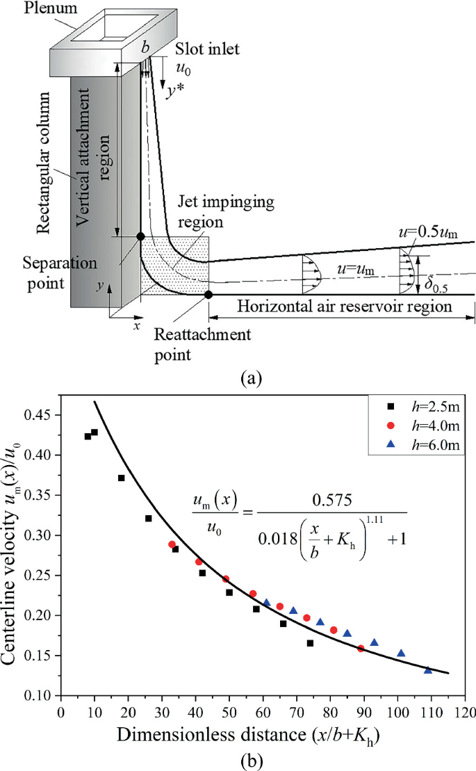

  

  Centerline velocity decay in the horizontal air reservoir region of RCAV. a Characteristic parameters, b dimensionless centerline velocity

Compared with Figs. 3.11 and 3.12, the velocity in the horizontal air reservoir region decays slower than that of the vertical attachment region. The centerline velocity decay in the horizontal air reservoir region is given by

$$\frac{{u_{\text{m}} \left( x \right)}}{u_0 } = \frac{0.575}{{0.018\left( {\frac{x}{b} + K_{\text{h}} } \right)^{1.11} + 1}}$$

(3.40)

where K_h is the height correction factor, $K_{\text{h}} { = }\frac{{1}}{{2}}\frac{h - 2.5}{b}$, the Cartesian coordinate system is shown in Fig. 3.11a.

3.4.2 Circular Column-Attached Jet

As mentioned above, circular column’s attachment ventilation is similar to rectangular column’s. The main difference between these two types of attachment ventilation is the circular column’s curvature effect. In the horizontal direction, the jet flow varies along the radial direction.

Eckert (2015) once pointed out that when the thickness of the fluid boundary layer δ is greater than or equal to the radius r of the circular column, the curvature effect should be taken into account. Nevertheless, for δ/r < 0.1, the curvature effect can be ignored. Mostly, δ/r < 0.1 in the practical engineering application, thus, the circular column-attached jet could be treated as a rectangular column or vertical wall-attached jet in the vertical attachment region.

• 1. Centerline velocity in the vertical attachment region

  For circular column attachment ventilation, the jet parameters in the vertical attachment region are shown in Fig. 3.13a. Figure 3.13b illustrates the dimensionless centerline velocity distribution under different slot heights, i.e., h = 2.5 m, 4.0 m, 6.0 m, and 8.0 m in the vertical attachment region. It can be seen from Fig. 3.13b that, in the range of 0 < y^*/b ≤ 45, the centerline velocity of the column-attached jet decays rapidly (decreasing almost linearly); while for y^*/b > 45, the centerline velocity decays relatively slow. Similar to the rectangular column attachment ventilation, the centerline velocity in the vertical attachment region can be expressed as Eq. (3.41)

  $$\frac{{u_{\text{m}} \left( {y^* } \right)}}{u_0 } = \frac{0.83}{{0.01\left( {\frac{y^* }{b}} \right)^{1.11} + 1}}$$

  (3.41)

  Fig. 3.13

  

  Centerline velocity in the vertical attachment region of CCAV. a Characteristic parameters, b dimensionless centerline velocity

• It should be noted that the column-attached jet will separate from the vertical wall when it is close to the floor. The separation point position is related to the slot height h. As h increases, the wall-attached jet will separate from the wall at a higher position. For h ≤ 4.0 m, such as ordinary office rooms, the height of the separation point is about 0.5 m; as h increases to 6.0 m, the position rises to about 1.0 m away from the floor.

• Centerline velocity in the horizontal air reservoir region

  For a circular column with a large curvature radius, the velocity decay in the horizontal air reservoir region is similar to that of the rectangular column, as shown in Fig. 3.14. The dimensionless centerline velocity decay also exhibits similarities, decreasing with the increase of x/b. The dimensionless centerline velocity distribution can be expressed by Eq. (3.42)

  $$\frac{{u_{\text{m}} \left( x \right)}}{u_0 } = \frac{0.575}{{0.035\left( {\frac{x}{b} + K_{\text{h}} } \right)^{1.11} + 1}}$$

  (3.42)

  Fig. 3.14

  

  Dimensionless centerline velocity decay in the horizontal air reservoir region of CCAV. a Characteristic parameters, b dimensionless centerline velocity

  where K_h is the height correction factor, $K_{\text{h}} { = }\frac{{1}}{{6}}\frac{h - 2.5}{b}$.

It should be pointed out that Eq. (3.42) is only applicable to the horizontal air reservoir region.

3.5 Velocity Distributions with Different Attachment Ventilation Modes

In order to have a deeper understanding of the similarities and differences between the VWAV, RCAV, and CCAV in nature, this section compares the centerline velocity distributions among those attachment ventilation modes.

3.5.1 Comparison of Centerline Velocity in Vertical Attachment Region

As shown in Fig. 3.15, in the vertical attachment region, there are similarities among the centerline velocity profiles of vertical wall-attached, rectangular column-attached, and circular column-attached jets. The dimensionless centerline velocities decrease exponentially as the distance y^*/b increases. The centerline velocity in the vertical attachment region can be expressed as a unified Eq. (3.43) with a relative error of less than 10%. For most ventilation engineering applications, Eq. (3.43) provides sufficient accuracy.

$$\frac{{u_{\text{m}} \left( {y^* } \right)}}{u_0 } = \frac{1}{{0.013\left( {\frac{y^* }{b}} \right)^{1.11} + 1}}$$

(3.43)

Fig. 3.15

Comparison of dimensionless centerline velocities in the vertical attachment region

3.5.2 Comparison of Centerline Velocity in Horizontal Air Reservoir Region

In the horizontal air reservoir region, there are significant differences among the three attachment ventilation’s centerline velocity distributions. As shown in Fig. 3.16, the velocity profiles reflect the influence of the attached wall on the velocity decay. When x/b + K_h ≤ 40, the VWAV’s centerline velocity decays slowest, followed by the RCAV, and the quickest for the CCAV. For x/b + K_h > 40, the velocity decay becomes slower than it would be in the range of x/b + K_h ≤ 40. In this range, the VWAV’s centerline velocity maintains the highest, the middle for the RCAV, and the lowest for the CCAV. The primary reason is that, for a rectangular column, the arris edges lead to the merging and superposition of airflow, which causes further momentum decay. Accordingly, for circular columns, particularly those with smaller diameters, the curvature effect exerts a remarkable influence on velocity decay.

Fig. 3.16

Comparison of dimensionless centerline velocities in the horizontal air reservoir region

We can conclude that the centerline velocity decays of all three attachment ventilations depend upon the shape factor C of the wall-attached jet and determined semi-empirical equations for the horizontal air reservoir region, which can be generally expressed as Eq. (3.44)

$$\frac{{u_{\text{m}} \left( x \right)}}{u_0 } = \frac{0.575}{{C\left( {\frac{x}{b} + K_{\text{h}} } \right)^{1.11} + 1}}$$

(3.44)

where C is shape factor, C = 0.0075 for VWAV, C = 0.0180 for RCAV, and C = 0.0350 for CCAV. K_h is the height correction factor, see Sects. 3.3 and 3.4.

The parameter correlations of vertical wall, rectangular column, and circular column attachment ventilation are summarized in Table 3.2.

Table 3.2 Correlations of various characteristic parameters of attachment ventilation air distribution

References

ANSI/ASHRAE Standard 113-2013 (2013) Method of testing for room air distribution. American Society of Heating, Refrigeration and Air-Conditioning Engineers Inc., Atlanta
ASHRAE (2017) ASHRAE handbook: fundamentals. American Society of Heating, Refrigeration and Air-Conditioning Engineers Inc., Atlanta
Eckert HU (2015) Simplified treatment of the turbulent boundary layer along a cylinder in compressible flow. J Aeronaut Sci 19(1):23–28
Eckert ERG, Drake RM Jr (1972) Analysis of heat and mass transfer. McGraw Hill, New York
Glauert MB (1956) The wall jet. J Fluid Mech 1(6):625–643
Li AG (2019) Extended Coanda effect and attachment ventilation. Indoor Built Environ 28(4):437–442
Prandtl L (1942) Bemerkungenzur Theorie der freien Tubulenz. J Appl Math Mech 22:241–243
Schwarz WH, Cosart WP (1961) The two-dimensional turbulent wall jet. J Fluid Mech 10(4):481–495
Sun DX (1992) Theoretical analysis of turbulent flow frictional resistance inside ducts of arbitrary angular cross sections. J Hydrodynam B 1:35–45
Verhoff A (1963) The two-dimensional turbulent wall jet without an external free stream. Princeton University
Zhang H (2011) Theoretical analysis and solution on flow field of indoor confined jet ventilation. Xi’an University of Architecture and Technology, Xi’an (in Chinese)
Author information
Authors and Affiliations
Corresponding author
Rights and permissions
Open Access This chapter is licensed under the terms of the Creative Commons Attribution-NonCommercial-NoDerivatives 4.0 International License (http://creativecommons.org/licenses/by-nc-nd/4.0/), which permits any noncommercial use, sharing, distribution and reproduction in any medium or format, as long as you give appropriate credit to the original author(s) and the source, provide a link to the Creative Commons license and indicate if you modified the licensed material. You do not have permission under this license to share adapted material derived from this chapter or parts of it.
The images or other third party material in this chapter are included in the chapter's Creative Commons license, unless indicated otherwise in a credit line to the material. If material is not included in the chapter's Creative Commons license and your intended use is not permitted by statutory regulation or exceeds the permitted use, you will need to obtain permission directly from the copyright holder.
Copyright information
© 2023 The Author(s)
About this chapter
Cite this chapter
Li, A. (2023). Isothermal Attachment Ventilation Mechanisms. In: Attachment Ventilation Theory. Springer, Singapore. https://doi.org/10.1007/978-981-19-9259-9_3
Download citation
DOI: https://doi.org/10.1007/978-981-19-9259-9_3
Published:
Publisher Name: Springer, Singapore
Print ISBN: 978-981-19-9258-2
Online ISBN: 978-981-19-9259-9
eBook Packages: EngineeringEngineering (R0)