Derivatives and Corporate Finance

Abstract

This chapter discusses how forward and futures contracts and options are related to corporate finance.

Appendix: Do Arbitrage When System 2 of the Gordan Theorem Fails

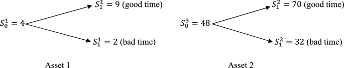
Assume a one-period, two states (good time and bad time) of nature world with no transaction costs (i.e., a perfect market). There are two assets: a money market (Security 1) which provides $1+0.25$ dollars at $t=1$ if one dollar is invested at $t=0$ (i.e., the risk-free interest rate is $r=0.25$), and two other securities (Security 2 and Security 3) with current market prices $4 and $48, respectively, which at $t=1$ provide:

That is, at $t=1$, when Security 2 provides $8, Security 3 will provide $70; and when Security 2 provides $2, Security 3 will provide $30. In this case, the two securities are not governed by the same probability measure (i.e., System 2 of the Gordan (Arbitrage) Theorem has no solution):

$$\left\{ {\begin{array}{*{20}l} {{\text{Security 1:}}\quad S_{0}^{1} = 1 = \frac{1}{1 + 0.25}\left( {\pi \times 1.25 + \left( {1 - \pi } \right) \times 1.{25}} \right){; }} \hfill \\ {{\text{Security 2:}}\quad S_{0}^{2} = 4 = \frac{1}{1 + 0.25}\left( {\frac{1}{2} \times 8 + \frac{1}{2} \times 2} \right);\quad {\varvec{p}}^{\prime } = \left[ {\begin{array}{*{20}c} {1/2} \\ {1/2} \\ \end{array} } \right] } \hfill \\ {{\text{Security 3:}}\quad S_{0}^{3} = 48 = \frac{1}{1 + 0.25}\left( {\frac{3}{4} \times 70 + \frac{1}{4} \times 30} \right);\quad {\varvec{p}}^{\prime \prime } = \left[ {\begin{array}{*{20}c} {3/4} \\ {1/4} \\ \end{array} } \right] } \hfill \\ \end{array} } \right.$$

i.e., we cannot find a vector ${\varvec{p}}=\left[\begin{array}{c}\pi \\ 1-\pi \end{array}\right]$, $0\le \pi \le 1$, such that System 2 holds:

$$\left[ {\begin{array}{*{20}l} {1.25 - 1\left( {1 + 0.25} \right)} \hfill & {{1}{\text{.25}} - 1\left( {1 + {0}{\text{.25}}} \right)} \hfill \\ {8 - 4\left( {1 + 0.25} \right)} \hfill & {{2} - 4\left( {1 + {0}{\text{.25}}} \right)} \hfill \\ {70 - 48\left( {1 + 0.25} \right)} \hfill & {{30} - 48\left( {1 + {0}{\text{.25}}} \right)} \hfill \\ \end{array} } \right]\left[ {\begin{array}{*{20}l} \pi \hfill \\ {1 - \pi } \hfill \\ \end{array} } \right] \ne \left[ {\begin{array}{*{20}c} 0 \\ 0 \\ 0 \\ \end{array} } \right].$$

By System 1 of the Arbitrage Theorem, there must exist an arbitrage opportunity. For example, at$t=0$, we can short sell one share of Security 3 and buy 5 shares of Security 2 and invest $28 $(=48-4\times 5)$ in the money market, and at $t=1$ we can earn excess profits, i.e.,

$$\left[ {\begin{array}{*{20}c} {1.25 - 1\left( {1 + 0.25} \right)\quad 8 - 4\left( {1 + 0.25} \right)\quad 70 - 48\left( {1 + 0.25} \right) } \\ {1.25 - 1\left( {1 + 0.25} \right)\quad {2} - 4\left( {1 + {0}{\text{.25}}} \right)\quad {30} - 48\left( {1 + {0}{\text{.25}}} \right)} \\ \end{array} } \right]\left[ {\begin{array}{*{20}c} x \\ 5 \\ { - 1} \\ \end{array} } \right]\left[ {\begin{array}{*{20}c} 5 \\ {15} \\ \end{array} } \right] > \left[ {\begin{array}{*{20}c} 0 \\ 0 \\ \end{array} } \right].$$

When investors adopt this arbitrage strategy at $t=0$, the market price of Security 2 will go up and that of Security 3 will go down. In equilibrium (i.e., no arbitrage), the market prices of the two securities at $t=0$ will adjust to the point that they all are priced by the same probability measure, say, ${\varvec{p}}=\left[\begin{array}{c}2/3\\ 1/3\end{array}\right]$,

$$\left\{ {\begin{array}{*{20}l} {{\text{Money Market}}\left( {{\text{Security}}\;{1}} \right){:}} \hfill & {S_{0}^{1} = {1} = \frac{1}{1 + 0.25}\left( {\frac{2}{3} \times { 1}{\text{.25}} + \frac{1}{3} \times {1}{\text{.25}}} \right)} \hfill \\ {\text{Security 2:}} \hfill & {S_{0}^{2} = 4.8 = \frac{1}{1 + 0.25}\left( {\frac{2}{3} \times 8 + \frac{1}{3} \times 2} \right)} \hfill \\ {\text{Security 3:}} \hfill & {S_{0}^{3} = 45\frac{1}{3} = \frac{1}{1 + 0.25}\left( {\frac{2}{3} \times 70 + \frac{1}{3} \times 30} \right)} \hfill \\ \end{array} } \right.$$

or

$$\begin{aligned} & \left[ {\begin{array}{*{20}c} {1.25 - 1\left( {1 + 0.25} \right)} & {{1}{\text{.25}} - 1\left( {1 + {0}{\text{.25}}} \right)} \\ {8 - 4.8\left( {1 + 0.25} \right)} & {{2} - 4.8\left( {1 + {0}{\text{.25}}} \right)} \\ {70 - 45\frac{1}{3}\left( {1 + 0.25} \right)} & {{30} - 45\frac{1}{3}\left( {1 + {0}{\text{.25}}} \right)} \\ \end{array} } \right]\left[ {\begin{array}{*{20}c} {2/3} \\ {1/3} \\ \end{array} } \right] = \left[ {\begin{array}{*{20}c} 0 \\ 0 \\ 0 \\ \end{array} } \right]. \\ & \begin{array}{*{20}c} {} & {} & {\quad {\varvec{A}}^{{\varvec{t}}} } & {} & {\quad \quad \quad \quad \quad \quad \quad \quad \quad {\varvec{p}}} & { = {\mathbf{0}}} \\ \end{array} \\ \end{aligned}$$

Since, in the above equation, the rank of the matrix ${\varvec{A}}$ is: $1 = m - 1$, the market is complete, and the probability measure ${\varvec{p}} = \left[ {\begin{array}{*{20}c} \pi \\ {1 - \pi } \\ \end{array} } \right] = \left[ {\begin{array}{*{20}c} {2/3} \\ {1/3} \\ \end{array} } \right]$ must be unique. In this example, $\frac{\pi }{1 - \pi } = \frac{2}{1}$ can be termed as the relative price ratio between the two states, i.e., at $t = 1$ the value of one dollar of good time is 200% greater than that of bad time. This implies that investors (the market) believe that the probability of good time is twice as many as that of bad time.

Problems

• 1. Comment on the following statements¹⁷:

  • (a) Wilmott (2007, p. 77): Assume: “(1) two stocks A and B; (2) both have the same value, same volatility and are denominated in the same currency; (3) both have call options with the same strike and expiration; (4) stock A is doubling in value every year, stock B is halving. Therefore, both call options have the same value. But which will you buy? That one stock is doubling and the other halving is irrelevant. That option prices don’t depend on the direction that the stock is going can be difficult to accept initially”.

  • (b) Ross (1998, p. 701): “Take two stocks that both follow binomial processes and that are not perfectly correlated. Further, suppose that the stocks differ only in that one has a much higher probability of an up jump than does the other. If our analysis is to be believed, then when the stock prices of each are equal the two option values will be equal! How can this be? How can the value of an option on a stock be independent of the probability that the stock will go up?”.

• 2. With zero interest rate, do the arbitrage for the following two assets:

  

• 3. Explain under what conditions an American put option will not be early exercised. How to use these conditions to determine the best time to liquidate a firm?

• 4. Explain how to use the p-index to invest in stocks. What are the limitations of the p-index?

• 5. Explain why the Black–Scholes-Merton option pricing model has: $\frac{\partial c}{{\partial \sigma }} = \frac{\partial p}{{\partial \sigma }}$ and the binomial option pricing model has: $\frac{\partial c}{{\partial u}} = \frac{\partial p}{{\partial u}}$ and $\frac{\partial c}{{\partial d}} = \frac{\partial p}{{\partial d}}$.

References

Black, F., & Scholes, M. (1973). The pricing of options and corporate liabilities. Journal of Political Economy, 81, 637–654.
Chang, K.-P. (2014). Some misconceptions in derivative pricing. http://ssrn.com/abstract=2138357.
Chang, K.-P. (2015). The ownership of the firm, corporate finance, and derivatives: Some critical thinking. Springer Nature.
Chang, K.-P. (2016). The Modigliani-Miller second proposition is dead; long live the second proposition. Ekonomicko-manažerské Spektrum, 10, 24–31. http://ssrn.com/abstract=2762158.
Chang, K.-P. (2017). On using risk-neutral probabilities to price assets. http://ssrn.com/abstract=3114126
Chang, K.-P. (2023). Measuring risk structures of assets: p-index and c-index. http://ssrn.com/abstract=4352457
Chang, K.-P. (2020). On option Greeks and corporate finance. Journal of Advanced Studies in Finance, 11, 183–193. https://doi.org/10.14505/jasf.v11.2(22).09
Cox, J., Ross, S., & Rubinstein, M. (1979). Option pricing: A simplified approach. Journal of Financial Economics, 7, 229–263.
Fama, Eugene and Michael Jensen. (1983). Agency problems and residual claims. Journal of Law and Economics, 26, 327–349.
Hull, J. (2018). Options, futures, and other derivatives. Pearson Education Limited.
Merton, R. (1973a). Theory of rational option pricing. Bell Journal of Economics and Management Science, 4, 141–183.
Merton, R. (1973b). The relationship between put and call option prices: Comment. Journal of Finance, 28, 183–184.
Myers, S. (1984). The search for optimal capital structure. Midland Corporate Finance Journal, 1, 6-16; also in Stern, J. M., & Chew, D.H., Jr. (Eds.). (1986). The revolution in corporate finance (pp. 91-99). Basil Blackwell
Stoll, H. (1969). The relationship between put and call option prices. Journal of Finance, 24, 801–824.
Author information
Authors and Affiliations
Corresponding author