Mixed-Criticality Scheduling on 5G New Radio

Abstract

Compared to industrial wired networks, 5G can improve device mobility and reduce the cost of networking. However, the real-time performance and reliability of 5G NR (new radio) still need to be improved to satisfy industrial applications’ requirements. In factories, the main factor that affects the performance of 5G NR is the unstable signal quality caused by high temperatures and metal. Although assigning dedicated resources to all transmissions and retransmissions is an effective method to improve the performance of 5G NR, the unstable signal quality causes the resources required for retransmissions to be uncertain. To address the problem, we introduce the mixed-criticality task model to 5G NR. When high-criticality packets cannot be transmitted, they are allowed to preempt the resources shared with low-criticality packets. The mixed-criticality scheduling problem of 5G NR is NP-hard. We formulate it as an OMT (optimization modulo theories) specification and propose a scheduling algorithm based on bin packing methods to make 5G NR satisfy industrial applications’ requirements. Finally, we conduct extensive evaluations based on an industrial 5G testbed and random test cases. The evaluation results indicate that our algorithm makes communication reliability greater than 99.9% on unlicensed spectrum, and for most test cases, our algorithm is close to optimal solutions.

6.1 Background

Ultra reliable low latency communication (URLLC) is one of main application areas defined in 5G. It aims to provide low latency and ultra-high reliability for mission-criticality services, which widely exist in industrial systems. Since the performance of URLLC is comparable to some wired networks, industrial systems are adopting 5G in place of wired networks to improve the mobility of devices and reduce the cost of networking [1,2,3].

For URLLC, all transmissions and retransmissions of industrial data must be assigned the resources of 5G NR (new radio), in advance, by a scheduling algorithm that runs in the base station. The resources of 5G NR include time slots and frequency bandwidth. In factories, high temperatures, high humidity, and metal seriously affect signal qualities. Thus, more retransmissions are needed to guarantee the reliability of industrial communications. However, on the one hand, the signal quality is dynamic and unpredictable. Before data packets are actually transmitted, the scheduling algorithm cannot determine how many retransmissions and network resources are sufficient for the highly reliable communications. On the other hand, the scheduling algorithm cannot assign as many resources as possible to all packets because wireless network resources are limited. Therefore, in order to make 5G NR meet the real-time and reliability requirements of industrial systems, the scheduling problem of 5G NR needs to be studied.

5G NR supports two-dimensional (2D) time-frequency resources. Since the 2D resources are different from other systems, some researchers have begun to study the new scheduling problems for 5G. The work in [4] proves the NP hardness of the new problem and proposes an algorithm based on Lagrangian duality to guarantee the real-time performance of as many services as possible. The work in [5] aims at the same objective and proposes two heuristic algorithms to generate schedules quickly. The work in [6] applies machine learning to improve real-time performance and data rate. Similarly, the work in [7], based on machine learning, proposes an energy-efficient real-time scheduling algorithm. To make the proposed algorithms usable in actual systems, some real factors have been considered. The work in [8] considers the on-off operation of power amplifiers in the scheduling problem and proposes a sliding window-based algorithm to optimize the real-time performance and the energy efficiency for service transmissions. The work in [9] focuses on the impact of interference and channel estimation error on data rate. The work in [10, 11] studies how to guarantee the delay requirement under the minimum bandwidth. Although the scheduling problem of 5G NR has been studied more and more widely, the mixed-criticality scheduling problem of 5G NR has not been considered.

In industrial systems, control commands are the most important and must be delivered to devices in time, while some less important data, such as system logs and routine monitoring, can be delayed. Hence, under the limitation of 5G NR, the best way to schedule packets is to assign more resources to important packets, and allow the other packets to use the rest of the resources and the idle resources that have been assigned to the finished important packets. In other words, when the resources of 5G NR are insufficient, unimportant packets have to be discarded first. This process is typical of mixed-criticality scheduling. Some novel algorithms have been proposed to address the mixed-criticality scheduling problems of networks [12,13,14,15,16,17]. However, these algorithms cannot be used in the 5G NR model.

In this chapter, we introduce mixed criticality to 5G NR and propose a mixed-criticality scheduling algorithm to improve the real-time performance and reliability of industrial 5G networks. Much research has focused on mixed-criticality scheduling algorithms. However, the two main characteristics of our problem are not considered in other research.

• 1. On 5G NR, the available resources include time slots and frequency bandwidth, while in other mixed-criticality systems, the resources are time slots and processors. Compared to processors, frequency bandwidth is finer-grained and can be divided and converged. Although this characteristic contributes to the flexibility of scheduling algorithms, it also makes scheduling algorithms more complicated and more difficult to find optimized solutions.

• 2. In related work about mixed-criticality networks, e.g., [18, 19], when high-criticality packets are transmitting, all the low-criticality packets have to be discarded. However, our scheduling algorithm tries to guarantee the performance of all the high- and low-criticality packets. This difference makes us have no related work to refer to.

To solve the mixed-criticality scheduling problem of 5G NR, this chapter includes the following:

• 1. First, to rigorously state the problem, we propose a specification based on optimization modulo theories (OMT). The problem can be reduced to the bin packing problem. Therefore, our problem is at least NP-hard. Based on the specification, some off-the-shelf solvers can find optimal solutions.

• 2. Second, to improve the scalability of our work, we propose a heuristic, pseudolevel-packing algorithm to assign dedicated and shared resources to packets. In the algorithm, we extend real-time constraints and mixed criticality to the traditional bin packing problem, and analyze the sufficient condition and necessary condition for schedulability so that the solution space can be reduced effectively.

• 3. Third, we implement an industrial 5G testbed and evaluate our proposed algorithms. To compare all the algorithms under the same signal quality, we record signal qualities into trace files. Then, we conduct simulations based on the trace files and extensive test cases. The results indicate that our algorithm makes communication reliability greater than 99.9% on unlicensed spectrum, and for most test cases, our proposed algorithm is close to optimal solutions.

6.2 Problem Statement

The symbols used in this chapter are summarized in Table 6.1.

Table 6.1 Symbols

We consider the scheduling problem under one base station and many users. A data flow is from a user to the base station (or from the base station to a user). In the following, we ignore the direction of flows because flows in different directions have the same resource requirement. In the flow set F, all flows have the same period P. Each flow f _i generates a packet at time j × P ($j\in \mathbb {Z}$), and the packet must be delivered to its destination before its absolute deadline (j + 1) × P. Since the packets contained in different periods have the same resource requirements, we only consider how to schedule packets in the first period P. After the first period, the subsequent schedules are periodically repeated.

Flow f _i is characterized by a three-tuple < χ _i, C _i, l _i > , which denotes its highest criticality level, transmission time durations and frequency bandwidth, respectively. The highest criticality level of our network is set to X, and for each f _i, 1 ≤ χ _i ≤ X. We use F ^e to denote the set of the flows with χ _i = e. The packet generated by f _i is τ _i. $C_i = \{c^1_i,c^2_i,\ldots ,c^{\chi _i}_i\}$ is the set of transmission time durations of τ _i. The flow with larger χ _i can occupy more time slots. At criticality level 1, τ _i is transmitted once in one time slot, and at criticality level j, τ _i is transmitted j times in j time slots, i.e., $c^j_i =j \times c^1_i$. 5G numerology defines three subcarrier spacings (180, 360 and 720 kHz) and three corresponding slot lengths (1000, 500 and 250 μs). We define 15 kHz and 250 μs as the unit bandwidth and the unit slot length, respectively. Then, $(l_i, c^1_i) \in \{(1,4),(2,2),(4,1)\}$ (as shown in Fig. 6.1a). We use x _i and y _i to denote the start time and start frequency of the transmission of τ _i, respectively. The illustration is shown in Fig. 6.1b. Initially, at the lowest criticality level, τ _i is transmitted once in time duration $c^1_i$. If τ _i is not sent successfully in the duration, then its critically level is set to 2. At criticality level 2, the transmission time duration is increased to $c^2_i$, and τ _i is transmitted again. Repeat this process until the transmission is successful. If the transmission still fails in the longest transmission time duration $c^{\chi _i}_i$, τ _i has to be discarded.

Fig. 6.1

Flow model. (a) (l _i,$c^1_i$) at criticality level 1. (b) τ _i at multiple criticality levels

For any two packets τ _i and τ _j, the resources assigned to them are not allowed to overlap each other (Definition 6.1). An example is shown in Fig. 6.2. At criticality level 2, the two packets share resources. Then, τ _j may be preempted by τ _i. At the same criticality level, the packets are equally important and cannot preempt each other. Therefore, in feasible solutions, packet overlapping is not allowed.

Fig. 6.2

Two packets overlap each other

Definition 6.1

τ _j and τ _i overlap each other (as shown in Fig. 6.2), if the following conditions are all met.

• 1. On the x axis (time dimension), τ _i and τ _j overlap, i.e., $x_i \le x_j \le x_i+c^{\min \{\chi _i,\chi _j\}}_i$ or $x_i \le x_j+c^{\min \{\chi _i,\chi _j\}}_j \le x_i+c^{\min \{\chi _i,\chi _j\}}_i$. We only check the highest criticality level occupied by both of them, i.e., $\min \{\chi _i,\chi _j\}$. At the other lower criticality levels, they occupy fewer time slots. Even if they do not overlap at the lower criticality levels, they may overlap at criticality level $\min \{\chi _i,\chi _j\}$.

• 2. On the y axis (frequency dimension), τ _i and τ _j overlap, i.e., y _i ≤ y _j ≤ y _i + l _i, or y _i ≤ y _j + l _j ≤ y _i + l _i.

If τ _i covers τ _j (Definition 6.2), τ _j may not be sent. As shown in Fig. 6.3, when τ _i is being transmitted at criticality level 3, the resources assigned to τ _j are being occupied by τ _i. Then, τ _j has to be discarded.

Fig. 6.3

τ _i covers τ _j

Definition 6.2

τ _i covers τ _j (as shown in Fig. 6.3), if the following conditions are all met.

• 1. τ _i and τ _j do not overlap each other (Definition 6.1).

• 2. The highest criticality level of τ _i is larger than that of τ _j, i.e., χ _i > χ _j.

• 3. On the x axis (time dimension), τ _i and τ _j share the same time slots at the different criticality levels, i.e., $x_i \le x_j \le x_i+c^{\chi _i}_i$, or $x_i \le x_j +c^{\chi _j}_j \le x_i +c^{\chi _i}_i$.

• 4. On the y axis (frequency dimension), τ _i and τ _j share the same frequency bandwidth, i.e., y _i ≤ y _j ≤ y _i + l _i, or y _i ≤ y _j + l _j ≤ y _i + l _i.

Our objective is to send as many packets as possible. Once a packet is covered, it may be discarded. If there are sufficient resources, no packets can be covered. For example, x _j is set to $x_i + c^{\chi _i}_i$ (as shown in Fig. 6.4). Then, τ _i and τ _j do not cover or overlap each other. No matter which criticality level τ _i is at, τ _j is not affected. Only when resources are insufficient, τ _i is allowed to cover τ _j.

Fig. 6.4

Sufficient resources

We formulate our problem as an OMT specification [20]. OMT is an extension of satisfiability modulo theories (SMT), which has been widely used to determine whether a specification is satisfiable or not. In addition to OMT supporting all the operators of SMT, it can also find an optimal objective. Our problem is to send as many packets as possible under scheduling constraints. Therefore, OMT is the best choice for our problem. The solution found by OMT not only satisfies scheduling constraints but also maximizes the number of packets sent. In the following specification, ∧, ∨ and ¬ denote the logical operations of conjunction, disjunction and negation, respectively.

Each flow in F generates one packet. All the packets are included in the packet set Γ. These packets are transmitted in resources including a bandwidth of L and a time duration of P. The problem is how to determine (x _i, y _i) for each packet such that as many packets as possible are transmitted, and high-criticality packets are not covered as much as possible. Therefore, the objective is to minimize the weighted sum of the number of covered packets, as follows:

$$\displaystyle \begin{aligned} {} \min \sum_{\forall e \in [1,X]}(\omega^e \times \sum_{\forall \tau_i \in \Gamma^e}q_i), \end{aligned} $$

(6.1)

where q _i = 1 indicates that τ _i is covered by a higher-criticality packet, ω ^e is the weight of the e-th criticality level, and Γ^e includes the packets with χ _i = e, i.e., Γ^e = {τ _i|∀f _i ∈ F, χ _i = e}. In order to ensure that high-criticality packets are not covered as much as possible, we set that ω ¹ = 1 and ∀e ∈ [2, X], ω ^e =∑_{∀g ∈ [1,e−1]} ω ^g ×| Γ^g| + 1, i.e., ω ^e is greater than the weighted sum of all lower-criticality packets. Hence, to minimize the objective, when there are not sufficient resources, low-criticality packets are covered first.

To check if τ _i and τ _j cover or overlap each other, we define the following function

(6.2)

The function only considers time-frequency resources, and criticality levels are reflected in c _i and c _j.

We use r _i,j to bridge q _i and Disjoint(). $\forall f_i \in F, \forall f_j \in \{F^{\chi _i+1},\ldots ,F^X\}$,

(6.3)

$$\displaystyle \begin{aligned} {} 1 \ge q_i \ge r_{i,j} \ge 0. \end{aligned} $$

(6.4)

In Eq. (6.3), if τ _j and τ _i cover or overlap each other, r _i,j is equal to 1. However, the following constraint 2) can avoid overlapping between two packets. Thus, only when τ _j covers τ _i, r _i,j = 1. Then, in Eq. (6.4), if there exists r _i,j = 1, then q _i = 1.

The minimizing problem has to respect the following constraints.

• 1. Range constraint: The ranges of variables used in the specification are as follows.

  

  (6.5)

• 2. Overlap constraint: Any two packets are not allowed to overlap each other. Note that in Eq. (6.6) the transmission time duration of τ _j is at the highest criticality level of τ _i because the overlap of two packets only occurs at the same level.

  $$\displaystyle \begin{aligned} {} \forall f_i \in F, \forall \tau_j \in \{\Gamma^e|\forall e \in [\chi_i,X]\}, Disjoint(i,c^{\chi_i}_i,j,c^{\chi_i}_j)=true. \end{aligned} $$

  (6.6)

A packet set is called schedulable if it has a feasible placement that meets all the constraints. When the objective is restricted to 0, the above problem is how to place all the packets into the rectangular area with dimensions L × P. This is the same as the 2D bin packing problem, in which a set of rectangular items is packed into a 2D rectangular bin. The NP-hardness of the 2D bin packing problem has been proven [21]. Since our problem can be reduced to the 2D bin packing problem, it is at least NP-hard. Hence, there is no polynomial time algorithm for finding an optimal solution. Although the specification (Eq. (6.1)–(6.6)) can be solved by OMT solvers, e.g. Z3, for complicated systems, the execution time of solvers cannot be acceptable. Therefore, in the following section, we will propose a heuristic algorithm to schedule packets.

6.3 Scheduling Algorithm

Firstly, we introduce a basic scheduling algorithm that does not consider the time constraint P and does not support any packet being covered. Secondly, based on the basic scheduling algorithm, we analyze the sufficient condition and necessary condition for schedulability. Finally, we extend the basic algorithm based on the two conditions to support time constraints and packet covering.

6.3.1 Basic Scheduling Algorithm

The basic scheduling algorithm is a pseudolevel-packing algorithm (as shown in Algorithm 6.1). Fig. 6.5 shows an illustration. There are two types of packing levels: super level and local level. A super level consists of multiple local levels. A local level is similar to the level that is widely used in multi-level bin packing algorithms, and its length is determined by the first packet placed at this local level. Algorithm 6.1 processes packets from the highest criticality level to the lowest criticality level (line 2). The packets with the same criticality level are placed at the same super level (lines 3–21). After all the packets in one criticality level are finished, a new super level is created to hold the packets in the next criticality level (lines 18–20). At each criticality level, the algorithm, first, sorts the packets according to the decreasing order of their transmission time durations (line 3), and then places packets in the same order (line 5). The single quotation mark on the symbols indicates that the symbols are sorted. For example, a sorted packet is denoted by $\tau ^{\prime }_i$, and its frequency bandwidth and transmission time duration are $l^{\prime }_i$ and $c^{\prime e}_i$, respectively. h is the finish time of all placed packets, and array a[ ][ ] is used to indicate which resources are occupied. If a[y][x] = 1, the resource at time slot x and on frequency y is occupied; otherwise, the resource is available. At each local level, the algorithm searches resources first in the order of time slots and then in the order of frequency (lines 6–15). If an available resource is found, i.e., a[y][x] = 0, the upper left corner of $\tau ^{\prime }_i$ is placed at coordinates (x, y) (line 16). The algorithm does not need to check all the resources that will be occupied by the rectangle of $\tau ^{\prime }_i$ because according to the above searching order, the other resources must be available as long as a[y][x] is available (Theorem 6.1). Then, based on the resources requested by $\tau ^{\prime }_i$, a[ ][ ] is updated (line 17). If there is not sufficient resource in the current local level, a new local level is created (lines 7 and 8). Repeat this process until all packets are placed. Finally, the locations of all the packets and the finish time are returned to the calling function. The time complexity of the algorithm is O(| Γ|Lh) because the algorithm traverses all the packets of Γ (lines 2 and 5) and all the resources of L × h (line 6). Since the basic scheduling does not support any packet being covered, the objective value is not considered in Algorithm 6.1.

Fig. 6.5

Illustration of Algorithm 6.1

Algorithm 6.1 Basic Scheduling Algorithm BasicSch( Γ)

Theorem 6.1

In the process of placing $\tau ^{\prime }_i$ , if a[y][x] = 0 and $y+l^{\prime }_i<L$ , then $\forall j \in [0,l^{\prime }_i),\forall k \in [0,c^{\prime \chi _i}_i)$ , a[y + j][x + k] = 0.

Proof

Assuming that $\exists \hat {y} \in (y,y+l^{\prime }_i), \exists \hat {x} \in (x,x+c^{\prime \chi _i}_i), a[\hat {y}][\hat {x}]=1$. Recall that 5G numerology defines only three subcarrier spacings, 15 kHz, 30 kHz, and 60 kHz. Thus, at a super level, there are three types of packets. We use B ¹, B ² and B ³ to denote them, and their widths and lengths are B ¹ = (l ¹, c ¹), B ² = (l ², c ²), and B ³ = (l ³, c ³), respectively. Based on the definition of three subcarrier spacings, we know that 4 × l ¹ = 2 × l ² = l ³ and c ¹ = 2 × c ² = 4 × c ³. Since $y+l^{\prime }_i<L$, the frequency resource is sufficient. Hence, we do not need to discuss the frequency dimension. We use row $\bar {y}$ to denote the last row above row y and occupied by some packets. In the following, we discuss the three cases of row $\bar {y}$.

• (1) There is no row $\bar {y}$ , and row y is the first row. However, in Algorithm 6.1, the first row of a local level is fully occupied because only when the first packet is placed is a new local level with the same length as the packet created. Therefore, the unoccupied a[y][x] is not at the first row, and row $\bar {y}$ must exist.

• (2) Row $\bar {y}$ is occupied by the same type of packets. The same type of packets cannot be two B ¹ because each local level contains at most one longest packet. If a[y][x] = 0 and $a[\hat {y}][\hat {x}]=1$, then the placement is shown in Fig. 6.6a. However, according to the searching order, the upper-left corner of the right packet should be at the point marked with a cross. Then, $a[\hat {y}][\hat {x}]$ is not occupied, i.e., $a[\hat {y}][\hat {x}]=0$.

  Fig. 6.6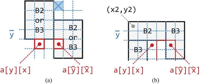

  

  Illustration of Theorem 6.1. (a) Illustration of Case (2). (b) Illustration of Case (3)

• (3) Row $\bar {y}$ is occupied by different types of packets. The different types of packets must be B ² and B ³. Since in Algorithm 6.1, the packets are sorted according to the decreasing order of their transmission time durations, the current packet $\tau ^{\prime }_i$ must be B ³. The illustration is shown in Fig. 6.6b. We know that c ² = 2 × c ³. Thus, two whole B ³ can be placed below B ². There is no other packet with different transmission time durations in this problem. Therefore, the packet that is not aligned with B ² does not exist, and $a[\hat {y}][\hat {x}]$ is not occupied, i.e., $a[\hat {y}][\hat {x}]=0$.

To sum up, $a[\hat {y}][\hat {x}]$ is not consistent with its definition. The above assumption does not hold. Therefore, $\forall \hat {y} \in (y,y+l^{\prime }_i), \forall \hat {x} \in (x,x+c^{\prime \chi _i}_i), a[\hat {y}][\hat {x}]=0$. □

6.3.2 Analysis

We, first, analyze the networks with only one criticality level, and then extend to multiple criticality levels. To simplify the description, when only one criticality level is considered, we ignore the symbols about criticality levels. In the networks with only one criticality level, the lengths of local levels can be c ¹, c ² or c ³, and L ≥ l ³. Assuming that in the result of Algorithm 6.1, there are n ¹, n ², and n ³ local levels with lengths of c ¹, c ², and c ³, respectively, and $n^1, n^2, n^3 \in \mathbb {N} \cap \{0\}$.

When only one criticality level is considered, Algorithm 6.1 has the following two properties.

Property 6.1

If n ¹ + n ² + n ³ = 1, and L approaches infinity, the resource utilization can be infinitesimal.

For example, there is only one packet in the network. Then, the resource utilization is $\frac {l_i \times c_i}{L \times c_i}$, which decreases as L increases.

Property 6.2

If n ¹ + n ² + n ³ > 1, the resource utilization must be greater than $\frac {1}{2}$.

Proof

To calculate the resource utilization, we need to analyze the amount of resources required by Algorithm 6.1 and the amount of resources actually occupied. The resources required by Algorithm 6.1 is E = L(n ¹ c ¹ + n ² c ² + n ³ c ³). The amount of resources actually occupied is analyzed in each of the following cases:

• (1) For the local levels with a length of c ¹, since the width of B ¹ is the unit width, in the first n ¹ − 1 local levels all the resources must be occupied. At the n ¹-th local level, if n ² = n ³ = 0, at least one B ¹ is placed, i.e., only l ¹ × c ¹ resources are occupied; if n ² ≠ 0, at most (l ² − 1) × c ¹ resources are idle because l ² × c ¹ resources are sufficient for the subsequent B ²; similarly, if n ² = 0 and n ³ ≠ 0, then (l ³ − 1) × c ¹ resources are idle. Thus, in the worst case, the amount of resources actually occupied in the n ¹ local levels is

  $$\displaystyle \begin{aligned} {R_1} = \left\{ \begin{array}{l} L{c^1}({n^1} - 1) + {l^1}{c^1},~\text{if}~{n^2} = {n^3} = 0~~~~~~~~(R_{1.1})\\ L{c^1}{n^1} - ({l^3} - 1){c^1},~\text{if}~{n^2} = 0,{n^3} \ne 0~~~~(R_{1.2})\\ L{c^1}{n^1} - ({l^2} - 1){c^1},~\text{others.}~~~~~~~~~~~~~~~~~~~(R_{1.3}) \end{array} \right.\end{aligned}$$

• (2) For the local levels with a length of c ², in the first n ² − 1 local levels, at most (Lmodl ²)c ²(n ² − 1) resources are idle. This is because after placing several B ², the last (Lmodl ²) rows are not enough for the next B ². At the n ²-th local level, if n ³ = 0, at least l ² c ² resources are occupied; otherwise, $\min \{(L-l^2),({l^3} - 1)\} c^2$ resources are idle because if L is very short, after placing B ², the remaining resources may be less than (l ³ − 1)c ². Thus, the amount of resources actually occupied in the n ² local levels is

  $$\displaystyle \begin{aligned} {R_2} = \left\{ \begin{array}{l} L{c^2}({n^2} - 1) - (L \mod l^2) \times {c^2}({n^2} - 1) + {l^2}{c^2}, ~~~\text{if}~{n^3} = 0~~~~(R_{2.1})\\ L{c^2}({n^2} -1) - (L \mod l^2) \times {c^2}({n^2} - 1) + L c^2 \\ - \min\{(L-l^2),({l^3} - 1)\} \times {c^2},~~~~~~~~~~~~~~~~~~~~~~~~~~~~~~~\text{others.}~~~(R_{2.2}) \end{array} \right.\end{aligned}$$

• (3) For the local levels with a length of c ³, R ₃ is similar to R ₂, i.e.,

  $$\displaystyle \begin{aligned} R_3=L c^3 (n^3 -1) - (L \mod l^3)\times c^3 (n^3-1) + l^3 c^3.\end{aligned}$$

Thus, the total amount of resources actually occupied is R = R ₁ + R ₂ + R ₃. Table 6.2 shows R and the lower bounds of utilization $\frac {R}{E}$ under different cases. The lowest bound in Table 6.2 is $\frac {1}{2}$. Therefore, the resource utilization must be greater than $\frac {1}{2}$. □

Table 6.2 Lower bound of resource utilization

Then, based on Properties 6.1 and 6.2, we analyze the sufficient condition for a packet set to be schedulable by Algorithm 6.1. Theorems 6.2 and 6.3 are about one criticality level and multiple criticality levels, respectively. In addition, the necessary condition for a packet set to be schedulable is shown in Theorem 6.4.

Theorem 6.2

For a packet set with only one criticality level, Algorithm 6.1 can find a feasible placement under the time constraint P, if $\max \{\max _{\forall \tau _i \in \Gamma }\{c_i\},\! \frac {2 \sum _{\forall \tau _i \in \Gamma } l_i \times c_i}{L}\} \le P$.

Proof

First, we discuss the placements with at least two local levels, i.e., n ¹ + n ² + n ³ > 1. In the proof of Property 6.2, R is the lower bound of resources actually occupied. Thus, the actual occupied resources $\sum _{\forall \tau _i \in \Gamma } l_i \times c_i$ is greater than or equal to R, i.e., $\sum _{\forall \tau _i \in \Gamma } l_i \times c_i \ge R > \frac {1}{2}E = \frac {1}{2}L(n^1 c^1 + n^2 c^2 + n^3 c^3)$. Rewriting, we obtain

$$\displaystyle \begin{aligned} \frac{2\sum_{\forall \tau_i \in \Gamma} l_i \times c_i}{L} > n^1 c^1 + n^2 c^2 + n^3 c^3. \end{aligned}$$

If $\frac {2\sum _{\forall \tau _i \in \Gamma } l_i \times c_i}{L} \le P$, then the actual length n ¹ c ¹ + n ² c ² + n ³ c ³ must be less than P, i.e., the placement is feasible under the time constraint P.

Then, from Property 6.1, we know that when n ¹ + n ² + n ³ = 1, $\frac {2\sum _{\forall \tau _i \in \Gamma } l_i \times c_i}{L}$ can be infinitesimal. However, the length of a local level is equal to the longest length of all the packets, i.e., $\max _{\forall \tau _i \in \Gamma }\{c_i\}$. Therefore, combining the above two cases, the sufficient condition is $\max \{\max _{\forall \tau _i \in \Gamma }\{c_i\}, \frac {2 \sum _{\forall \tau _i \in \Gamma } l_i \times c_i}{L}\} \le P$. □

Theorem 6.3 (Sufficient Condition)

For a packet set with multiple criticality levels, Algorithm 6.1 can find a feasible placement under the time constraint P, if

$$\displaystyle \begin{aligned} {} \sum_{\forall e \in [1,X]}(\max\{\max_{\forall \tau_i \in \Gamma^e}\{c^e_i\}, \frac{2 \sum_{\forall \tau_i \in \Gamma^e} l_i \times c^e_i}{L}\}) \le P. \end{aligned} $$

(6.7)

Proof

Since Algorithm 6.1 places super levels one by one, the total length is the sum of the lengths of all super levels. If the total length satisfies the time constraint P, the placement is feasible. □

Theorem 6.4 (Necessary Condition)

For a packet set with multiple criticality levels, if Algorithm 6.1 find a feasible placement for a packet set under the time constraint P, then the packet set satisfies the following condition:

$$\displaystyle \begin{aligned} {} \sum_{\forall \tau_i \in \Gamma} l_i \times c^{\chi_i}_i \le L \times P. \end{aligned} $$

(6.8)

Proof

Note that in Algorithm 6.1 high-criticality packets are not allowed to cover low-criticality packets. Thus, if a packet set is schedulable, its resource utilization cannot be greater than 100%, i.e., $\frac {\sum _{\forall \tau _i \in \Gamma } l_i \times c^{\chi _i}_i}{L \times P} \le 100\%$. □

6.3.3 Improved Algorithm

In this subsection, we design our scheduling algorithm based on Theorems 6.3 and 6.4. The objective of our problem is to cover as few packets as possible, and low-criticality packets are covered first. Hence, we sort the packets of Γ according to the following rules: ∀τ _i, τ _j ∈ Γ,

• if χ _i > χ _j, then τ _i is before τ _j in the ordered set Γ′;

• if χ _i = χ _j and $c^{\chi _i}_i > c^{\chi _j}_j$, then τ _i is before τ _j in the ordered set Γ′;

• if χ _i = χ _j, $c^{\chi _i}_i = c^{\chi _j}_j$ and i < j, then τ _i is before τ _j in the ordered set Γ′.

To optimize the objective, an effective method should cover the packets of Γ′ from back to front. First, no packet can be covered, and the current packet set is checked whether it is schedulable or not under the time constraint P. If the packet set is not schedulable, the last packet $\tau _{|\Gamma '|}$ is covered. Then, if the new packet set is still unschedulable, the packets $\tau _{|\Gamma '|-1}$ and $\tau _{|\Gamma '|}$ are covered. Repeat this process until a schedulable packet set is found. However, this method may traverse all the packets. To improve the efficiency of our algorithm, we reduce the solution space based on Theorems 6.3 and 6.4, and adopt binary search instead of linear search. In Theorem 6.5, we proved that the solutions corresponding to the sorted packets are also ordered. Thus, the binary search can be used in our scheduling problem.

Algorithm 6.2 Scheduling Algorithm with packet Covering (SAC)

Algorithm 6.3 Covering Algorithm Cover(k)

Our scheduling algorithm is shown in Algorithm 6.2. The variable k is used to denote that the packets after the k-th packet can be covered, and the function Cover(k) (Algorithm 6.3) is to determine which packets are selected to cover these packets. In Cover(k), for each packet $\tau ^{\prime }_i$ (i > k), the metric δ _j indicates the area difference between $\tau ^{\prime }_j$ and $\tau ^{\prime }_i$ in the time-frequency coordinate (line 8). If $\tau ^{\prime }_j$ cannot fully cover $\tau ^{\prime }_i$, it is not an available selection (line 4). This is because if a small packet covers a big one, then the overflowing part of the big packet will change the shape of the small packet, and the schedulability will become worse. Then, to reduce the waste of resources, the packet with the minimal δ _j is selected to cover $\tau ^{\prime }_i$ (lines 14–15), and the covered packet $\tau ^{\prime }_i$ is marked in Γ′ (line 16). If none of the packets have a valid δ _j, $\tau ^{\prime }_i$ cannot be covered even though it is allowed to be covered. Finally, Cover(k) returns Γ′ to Algorithm 6.2, called as $\Gamma ^{\prime }_k$.

Algorithm 6.2 traverses k from | Γ′| to 1 (lines 1, 3 and 7). The first k that makes $\Gamma ^{\prime }_k$ satisfy the necessary condition is the rightmost element of the binary search (lines 2–5), and then similarly, the first k that makes $\Gamma ^{\prime }_k$ satisfy the sufficient condition is the leftmost element (lines 6–9). Then, in the binary search, for each middle element, $BasicSch(\Gamma ^{\prime }_{middle})$ is invoked to place the packet set and returns the finish time. If the finish time is not greater than time P, a better solution may be between middle and right; otherwise, a feasible solution is between left and middle (lines 12–17). The leftmost element is always a feasible solution unless no packet set satisfies the sufficient condition. Thus, only when the leftmost element is 0, and the middle element does not search for any feasible solution, Γ cannot be scheduled (lines 19 and 20). Otherwise, the placement under the latest leftmost element is the final solution (line 22). In Algorithm 6.3, the number of iterations in lines 1, 2, 6 and 15 is O(| Γ′|), O(| Γ′|), O(X) and O(X), respectively. Thus, the time complexity of Algorithm 6.3 is O(| Γ′|² X). In Algorithm 6.2, the number of invoking Cover( ) is O(| Γ′|) in the worst case. Hence, the time complexity of lines 1–9 is O(| Γ′|³ X). Then, in lines 10–18, the number of invoking BasicSch( ) is $O(\log |\Gamma '|)$, and its time complexity is $O(\log |\Gamma '| \cdot |\Gamma '|Lh)$. Therefore, the time complexity of Algorithm 6.2 is O(n ⁴).

Theorem 6.5

If $\Gamma ^{\prime }_k$ can be placed before time P, so can $\Gamma ^{\prime }_{k-1}$ , and $Obj(\Gamma ^{\prime }_{k-1}) \ge Obj(\Gamma ^{\prime }_k)$ ; if $\Gamma ^{\prime }_k$ cannot be placed before time P, neither can $\Gamma ^{\prime }_{k+1}$ , and $Obj(\Gamma ^{\prime }_k) \ge Obj(\Gamma ^{\prime }_{k+1})$ , where $Obj(\Gamma ^{\prime }_k)$ is the objective value of packet set $\Gamma ^{\prime }_k$ calculated based on Eq.(6.1).

Proof

First, we prove that for our problem if $\Gamma ^{\prime }_k$ has a feasible solution, then $\Gamma ^{\prime }_{k-1}$ also has a feasible solution, and the objective value of $\Gamma ^{\prime }_{k-1}$ is not greater than that of $\Gamma ^{\prime }_k$. The difference between $\Gamma ^{\prime }_k$ and $\Gamma ^{\prime }_{k-1}$ is that $\tau ^{\prime }_k$ may be covered in $\Gamma ^{\prime }_{k-1}$, while it cannot be covered in $\Gamma ^{\prime }_k$. There are two cases:

• 1. When $\tau ^{\prime }_k$ is covered in $\Gamma ^{\prime }_{k-1}$, we discuss all types of $\tau ^{\prime }_k$ as follows: if $\tau ^{\prime }_k$ is B ¹, in the same local level, the places of the subsequent packets are moved from (x, y) to (x, y − l ¹); if $\tau ^{\prime }_k$ is B ², in the same local level, the places of the subsequent packets are moved from (x, y) to (x, y − l ²), (x − c ², y) or (x + c ², y − l ²); if $\tau ^{\prime }_k$ is B ³, in the same local level, the places of the subsequent packets are moved from (x, y) to (x − c ³, y) or (x + (the length of the local level) − 1, y − l ³). In these cases, the subsequent packets are moved up and left in the same local level. Therefore, the finish time of $\Gamma ^{\prime }_{k-1}$ is not later than that of $\Gamma ^{\prime }_{k}$. In addition, based on Eq. (6.1), if $\tau ^{\prime }_k$ is covered, $Obj(\Gamma ^{\prime }_{k-1}) =Obj(\Gamma ^{\prime }_k)+ \omega ^{\chi ^{\prime }_k}$.

• 2. When $\tau ^{\prime }_k$ is not covered in $\Gamma ^{\prime }_{k-1}$, $\Gamma ^{\prime }_k = \Gamma ^{\prime }_{k-1}$, i.e., they have the same solution, and $Obj(\Gamma ^{\prime }_{k-1}) =Obj(\Gamma ^{\prime }_k)$.

Therefore, if $\Gamma ^{\prime }_k$ can be placed before time P, so can $\Gamma ^{\prime }_{k-1}$, and $Obj(\Gamma ^{\prime }_{k-1}) \ge Obj(\Gamma ^{\prime }_k)$.

Second, for $\Gamma ^{\prime }_k$ and $\Gamma ^{\prime }_{k+1}$, $\tau ^{\prime }_{k+1}$ can be covered in $\Gamma ^{\prime }_k$, but cannot be covered in $\Gamma ^{\prime }_{k+1}$. Packet $\tau ^{\prime }_{k+1}$ introduces more delay into the solution of $\Gamma ^{\prime }_{k+1}$. Hence, if the finish time of $\Gamma ^{\prime }_k$ is greater than P, $\Gamma ^{\prime }_{k+1}$ cannot finish before time P. For the objective value, if $\tau ^{\prime }_{k+1}$ is covered in $\Gamma ^{\prime }_k$, $Obj(\Gamma ^{\prime }_k) = Obj(\Gamma ^{\prime }_{k+1}) + \omega ^{\chi ^{\prime }_{k+1}}$; otherwise, $Obj(\Gamma ^{\prime }_k) = Obj(\Gamma ^{\prime }_{k+1})$. Therefore, if $\Gamma ^{\prime }_k$ cannot be placed before time P, neither can $\Gamma ^{\prime }_{k+1}$, and $Obj(\Gamma ^{\prime }_k) \ge Obj(\Gamma ^{\prime }_{k+1})$. □

6.4 Performance Evaluations

In this section, we will evaluate our proposed algorithms based on a 5G testbed and extensive test cases. Five metrics are used in our evaluation: (1) packet loss ratio (PLR) is the ratio of the number of lost packets to the total number of sent packets; (2) schedulable ratio is the percentage of test cases for which an algorithm can find a feasible solution; (3) objective value is calculated based on Eq. (6.1); (4) execution time is the time required to find an optimized solution; and (5) the number of calls to BasicSch( ) reflects the effectiveness of Theorems 6.3 and 6.4.

Our proposed algorithm SAC is compared with the following methods:

• 1. OMT adopts the Microsoft solver Z3 [22] to solve our OMT specification (Eq. (6.1)–(6.6)). Although the solver can find the optimal solution, its execution time is unacceptable when the problem is complex. Thus, OMT only appears in simple test cases.

• 2. T4 corresponds to the necessary condition of Theorem 6.4. We need an excellent baseline to illustrate the effectiveness of our algorithm. However, there is no method to find optimal solutions for complicated test cases. Therefore, when Z3 cannot find optimal solutions in an acceptable time, we replace OMT with T4. In T4, if a test case satisfies Theorem 6.4, it is considered schedulable. Hence, for schedulable ratios, T4 is better than optimal solutions when packets do not cover each other. For the objective of the scheduling problem, if in an ordered set Γ′ the first k packets satisfy Theorem 6.4, we assume that the packets after these k packets are covered. Thus, the objective value of T4 is always better than optimal solutions. Note that T4 is an analysis-based method and cannot generate schedules. Hence, we do not consider its execution time and PLR.

• 3. FFDH (First-fit decreasing-height) [23] is a classical strip packing algorithm. In this chapter, FFDH sorts packets by order of non-increasing length, and then scans the local levels from left to right. Each packet is placed in the first level that has sufficient resources. FFDH does not support packet covering. Hence, we cannot calculate the original objective value of FFDH. The original objective value is about the covered packets. In FFDH, this kind of packets includes those that cannot be placed before P. Therefore, when some packets cannot be placed before P, they are used to calculate the objective value based on Eq. (6.1).

• 4. SACwoT3T4 is the same as SAC except that it does not adopt Theorems 6.3 and 6.4 to reduce the solution space.

All algorithms are written in C and run on a Windows workstation with a 3.7 GHz CPU and 64 GB memory. The parameters used in the evaluation are summarized in Table 6.3. In a test case, N packets are transmitted in a 3D space of dimensions X × L × P. For each packet, its criticality level is randomly selected in the range [1, X], and the transmission time duration at the lowest criticality level and bandwidth are randomly selected in {(1, 4), (2, 2), (4, 1)}.

Table 6.3 Parameters

6.4.1 Evaluations Based on A Real Testbed

In this subsection, we evaluate packet loss ratios of different algorithms. The other metrics are not affected by the signal quality, and are more suitable for being tested through extensive test cases, which are shown in the next subsection. Our 5G testbed is shown in Fig. 6.7. It operates in the 2.4 GHz unlicensed ISM (industrial scientific and medical) band. The licensed spectrum is managed by mobile network operators, and developers and users cannot modify any strategy. Therefore, we adopt the unlicensed spectrum. If the strategies on the licensed spectrum are allowed to be customized, our proposed algorithms can be used without modification. Two 5G devices [24] are configured as a base station and a user, respectively. Since the signal quality is dynamic and unknown, to guarantee fairness for all algorithms, we trace the states of 7 subcarriers and 60,000 time slots, and then conduct trace-driven simulations.

Fig. 6.7

5G testbed

First, in small networks, we compare SAC and OMT (as shown in Fig. 6.8). The parameter setting is < N, X, L, P >=< 10, 4, 7, 20 > , and CLx denotes the PLR at criticality level x. Since high-criticality packets can be transmitted more times, CL4 is the lowest. Both OMT and SAC successfully assign resources to the packets at criticality level 4. The average of CL4 in OMT and SAC are 0.072% and 0.067%, respectively. The slight difference between them is caused by the dynamics of signal quality. The average of CL1 in OMT and SAC are 16.7% and 17.0%, respectively. In SAC, since some low-criticality packets share resources with high-criticality packets, the CL1 of SAC is lower than that of OMT.

Fig. 6.8

Packet loss ratios in simple networks. (a) OMT. (b) SAC

Second, since OMT cannot solve complex problems in an acceptable time, we compare only SAC and FFDH in large networks (as shown in Fig. 6.9). The parameter setting is < 80, 4, 7, 80 > . Since the control period of the robotic arms in our testbed is 20 ms, and our 5G device supports 4 time slots in 1 ms, the parameter P is set to 80. FFDH reserves dedicated resources for packets. When high-criticality packets do not need to be retransmitted, the assigned resources are wasted, and low-criticality packets cannot obtain sufficient resources. Hence, the average of CL1 is about 70.9%. In addition, FFDH does not consider criticality levels so that some high-criticality packets are discarded. Therefore, FFDH has higher PLRs even at the highest criticality level. The average of CL4 in FFDH is about 17.2%. SAC makes the best of resources to guarantee the requirements of packets. Hence, the average of CL4 in SAC is 0.071%, and for CL1, when the PLR of FFDH is 70.9%, SAC improves PLR to 42.7%. In SAC, the PLR of the highest criticality level is still about 0.07%, no matter which networks SAC is used in. Thus, SAC makes communication reliability greater than 99.9% under real-time constraints.

Fig. 6.9

Packet loss ratios in complicated networks. (a) SAC. (b) FFDH

6.4.2 Evaluations Based on Random Test Cases

In the following, we will randomly generate extensive test cases to comprehensively evaluate the performance of our proposed algorithms. To make Z3 solvable, the parameter settings are < [10, 18], 4, 7, 20 > , and 12 processes run in parallel on our workstation. For each parameter setting, 200 test cases are randomly generated. The results are shown in Fig. 6.10. The objective value is the average of 200 test cases. As N increases, the schedulable ratios decrease, and the objective value increases because it is hard to find optimized solutions when more and more packets are transmitted on limited resources. The worst algorithm is FFDH. Since in FFDH, no packet can be covered, the limited resources are not sufficient to transmit all packets. OMT has the highest schedulable ratio and the lowest objective value. However, the execution time of OMT fluctuates greatly. For some simple test cases, Z3 cannot find solutions within 12 hours. Thus, we set the time limit of Z3 as 1 hour. The execution times are shown in Fig. 6.11. When N < 16, almost all test cases can be solved within the time limit; when N ≥ 16, about 80% of test cases can be solved. Among all these test cases, the shortest execution time of OMT is 127 ms. Such a long execution time makes the network unable to respond to burst packets. However, when SAC is used to solve the same test cases, the longest execution time is only 0.19 ms. Even for the complicated test cases used in the following evaluations, the execution time of SAC is less than 3.7 ms, and the amount of memory space required is less than 1.2 MB. Therefore, SAC can quickly respond to burst packets and improve the flexibility of industrial networks.

Fig. 6.10

Comparison with OMT. (a) Schedulable ratio. (b) Objective value

Fig. 6.11

Execution times of Z3. (a) N = 14. (b) N = 16. (c) N = 18

Then, we increase the complexity of test cases. The parameter settings in Fig. 6.12 are < [40, 100], 4, 10, 80 > . For each parameter setting, 1000 test cases are randomly generated. When N > 70, SAC has a higher schedulable ratio than T4 because SAC allows packets to share resources. Although this causes some low-criticality packets to fail to be sent, compared to FFDH, SAC discards only 34% of packets, i.e., SAC makes a trade-off between schedulability and reliability. Therefore, in a network with limited resources, to schedule more high-criticality packets, SAC is the best choice.

Fig. 6.12

Comparison under varying N. (a) Schedulable ratio. (b) Objective value

In Fig. 6.13, we change X to illustrate its effect on schedulable ratios and objective values. The parameter settings are < {60, 70}, {3, 4, 5}, 10, 80 > . To show the results more clearly, the objective values of SAC under N = 70 and X = 4 are displayed in Fig. 6.14. Due to the limited resources, some packets have to be covered. Hence, the objective values of some test cases are greater than zero. In Fig. 6.13, as X increase, the schedulable ratio decreases, and the objective value increases. This is because more retransmissions lead to a more serious lack of resources. Furthermore, if a test case contains more packets than others, it will be more severely affected by X. For example, Fig. 6.13b and d (N = 70) has greater fluctuations than Fig. 6.13a and c (N = 60). Thus, if there are many packets in a network, X should be carefully determined based on the signal quality and should be as small as possible.

Fig. 6.13

Comparison under varying X. (a) Schedulable ratio. (b) Schedulable ratio. (c) Objective (d) Objective

Fig. 6.14

The objective values of SAC under N = 70 and X = 4

The parameter settings in Figs. 6.15 and 6.16 are < 80, 4, [8, 16], 80 >  and < 80, 4, 10, [70, 95] > , respectively. As L and P increase, the schedulable ratio increases, and the objective value decreases. This is because the more resources, the easier it is to schedule packets. In Figs. 6.15 and 6.16, when their total resources are the same, their schedulable ratios and objective values are similar. For example, in Fig. 6.15, when L = 11, the amount of resources is 880, and the schedulable ratio and objective value are 95% and 56, respectively. In Fig. 6.16, if the amount of resources is 880, then P is 88. When P = 88, the schedulable ratio and objective value are 94% and 58, respectively. Therefore, L and P have similar effects on schedulability and reliability, i.e., if the time constraint P of an industrial system cannot be relaxed, we can improve the system performance by increasing L.

Fig. 6.15

Comparison under varying L. (a) Schedulable ratio. (b) Objective

Fig. 6.16

Comparison under varying P. (a) Schedulable ratio. (b) Objective

In Fig. 6.17, we compare SAC and SACwoT3T4. SACwoT3T4 adopts binary search to find solutions in the whole solution space. Compared to SACwoT3T4, SAC reduces the solution space based on Theorems 6.3 and 6.4. Thus, SAC can significantly decrease the number of calls to function BasicSch(). When N < 70, SAC can directly find the optimal solution for almost all test cases. Therefore, Theorems 6.3 and 6.4 are effective.

Fig. 6.17

Comparison between SAC and SACwoT3T4

6.5 Summary

This chapter focuses on the mixed-criticality scheduling problem of 5G NR. We present the mixed-criticality 5G NR model and formulate the problem as an OMT specification. Then, for the schedulability of the mixed-criticality scheduling problem, we analyze its sufficient condition and necessary condition. Based on the two conditions, we propose a scheduling algorithm. Finally, an industrial 5G testbed and extensive test cases are used to evaluate our proposed algorithm. The evaluation results indicate that our proposed algorithm can improve the real-time performance and reliability of 5G NR.

References

Huawei Technologies Co. Ltd. (2020) Unlocking the value of 5G industry applications. https://www.cio.com/article/3564155/unlocking-the-value-of-5g-industry-applications.html
5G Industry Campus Europe (2020) 5G industry campus use cases. https://5g-industry-campus.com/use-cases/
Cheng JF, Chen WH, Tao F, Lin CL (2018) Industrial IoT in 5G environment towards smart manufacturing. J Ind Inf Integration 10:10–19
You L, Liao Q, Pappas N, Yuan D (2018) Resource optimization with flexible numerology and frame structure for heterogeneous services. Commun Lett 22(12):2579–2582
Nguyen TT, Ha VN, Le LB (2019) Wireless scheduling for heterogeneous services with mixed numerology in 5G wireless networks. Commun Lett 24(2):410–413
Zhang JX, Xu XD, Zhang KJ, Zhang BF, Tao XF, Zhang P (2019) Machine learning based flexible transmission time interval scheduling for eMBB and URLLC coexistence scenario. IEEE Access 7:65811–65820
Lei L, You L, He Q, Vu TX, Chatzinotas S, Yuan D, Ottersten B (2019) Learning-assisted optimization for energy-efficient scheduling in deadline-aware NOMA systems. Trans Netw 3(3):615–627
Sui WS, Chen XJ, Zhang SQ, Jiang ZY, Xu SG (2019) Energy-efficient resource allocation with flexible frame structure for heterogeneous services. In: The international conference on internet of things and IEEE green computing and communications and IEEE cyber, physical and social computing and IEEE smart data. IEEE, Piscataway, pp 749–755
Marijanovic L, Schwarz S, Rupp M (2019) A novel optimization method for resource allocation based on mixed numerology. In: The IEEE international conference on communications, pp 1–6
Anand A, De Veciana G (2018) Resource allocation and HARQ optimization for URLLC traffic in 5G wireless networks. J Sel Areas Commun 36(11):2411–2421
Anand A, De Veciana G, Shakkottai S (2020) Joint scheduling of URLLC and eMBB traffic in 5G wireless networks. Trans Netw 28(2):477–490
Gavrilut V, Pop P (2020) Traffic-type assignment for TSN-based mixed criticality cyber-physical systems. Trans Cyber Phys Syst 4(2):1–27
Gavrilut V, Zhao L, Raagaard ML, Pop P (2018) AVB-aware routing and scheduling of time-triggered traffic for TSN. IEEE Access 6:75229–75243
Harbin JR, Griffin DJ, Burns A, Bate IJ, Davis RI, Indrusiak LS (2018) Supporting critical modes in AirTight. In: Embedded and Real-Time Computing Systems and Applications. IEEE, Piscataway, pp 7–12
Burns A, Harbin J, Indrusiak L, Bate I, Davis R, Griffin D (2018) AirTight: a resilient wireless communication protocol for mixed criticality systems. In: The International Conference on Embedded and Real-Time Computing Systems and Applications. IEEE, pp 65–75
Xia C, Jin X, Kong L, Zeng P (2017) Bounding the demand of mixed criticality industrial wireless sensor networks. IEEE Access 5:7505–7516
Jin X, Xia C, Xu H, Wang J, Zeng P (2016) Mixed criticality scheduling for industrial wireless sensor networks. Sensors 16(9):1376–1396
Novak A, Sucha P, Hanzalek Z (2016) Efficient algorithm for jitter minimization in time-triggered periodic mixed-criticality message scheduling problem. In: The international conference on real-time networks and systems, pp 23–31
Novak A, Sucha P, Hanzelek Z (2019) Scheduling with uncertain processing times in mixed-criticality systems. Eur J Oper Res 279(3):687–703
Kovasznai G, Biro C, Erdelyi B (2017) Generating optimal scheduling for wireless sensor networks by using optimization modulo theories solvers. In: The international workshop on satisfiability modulo theories, pp 15–27
Lodi A, Martello S, Monaci M (2002) Two-dimensional packing problems: a survey. Eur J Oper Res 141(2):241–252
Bjorner N, Phan AD (2014) vZ - Maximal Satisfaction with Z3. In: The 6th international symposium on symbolic computation in software science. pp 1–9
Coffman J, Edward G, Garey MR, Johnson DS, Tarjan RE (1980) Performance bounds for level-oriented two-dimensional packing algorithms. SIAM J Comput 9(4):808–826
Yunzhi Ruantong Ltd. (2021) 5G URLLC device user guide. http://yunzhiruantong.com/?m=home&c=View&a=index&aid=176
Author information
Authors and Affiliations
Rights and permissions
Open Access This chapter is licensed under the terms of the Creative Commons Attribution 4.0 International License (http://creativecommons.org/licenses/by/4.0/), which permits use, sharing, adaptation, distribution and reproduction in any medium or format, as long as you give appropriate credit to the original author(s) and the source, provide a link to the Creative Commons license and indicate if changes were made.
The images or other third party material in this chapter are included in the chapter's Creative Commons license, unless indicated otherwise in a credit line to the material. If material is not included in the chapter's Creative Commons license and your intended use is not permitted by statutory regulation or exceeds the permitted use, you will need to obtain permission directly from the copyright holder.
Copyright information
© 2023 The Author(s)
About this chapter
Cite this chapter
Jin, X., Xia, C., Xu, C., Li, D. (2023). Mixed-Criticality Scheduling on 5G New Radio. In: Mixed-Criticality Industrial Wireless Networks. Wireless Networks. Springer, Singapore. https://doi.org/10.1007/978-981-19-8922-3_6
Download citation
DOI: https://doi.org/10.1007/978-981-19-8922-3_6
Published:
Publisher Name: Springer, Singapore
Print ISBN: 978-981-19-8921-6
Online ISBN: 978-981-19-8922-3
eBook Packages: Computer ScienceComputer Science (R0)