Case Study IV: Tuned Reinforcement Learning (in Python)

Abstract

Similar to the example in Chap. 10, which considered tuning a Deep Neural Network (DNN), this chapter also deals with neural networks, but focuses on a different type of learning task: reinforcement learning. This increases the complexity, since any evaluation of the learning algorithm also involves the simulation of the respective environment. The learning algorithm is not just tuned with a static data set, but rather with dynamic feedback from the environment, in which an agent operates. The agent is controlled via the DNN. Also, the parameters of the reinforcement learning algorithm have to be considered in addition to the network parameters. Based on a simple example from the Keras documentation, we tune a DNN used for reinforcement learning of the inverse pendulum environment toy example. As a bonus, this chapter shows how the demonstrated tuning tools can be used to interface with and tune a learning algorithm that is implemented in Python.

1 Introduction

In this chapter, we will demonstrate how a reinforcement learning algorithm can be tuned. In reinforcement learning, we consider a dynamic learning process, rather than a process with fixed, static data sets like in typical classification tasks.

The learning task considers an agent, which operates in an environment. In each timestep, the agent decides to take a certain action. This action is fed to the environment, and causes a change from a previous state to a new state. The environment also determines a reward for the respective action. After that, the agent will decide the next action to take, based on received reward and the new state. The learning goal is to find an agent that accumulates as much reward as possible.

To simplify things for a second, let us consider an example: A mobile robot (agent) is placed in a room (environment). The state of the agent is the position of the robot. The reward may be based on the distance traveled toward a target position. Different movements of the robot are the respective actions.

In this case, our neural network can be used to map from the current state to a new action. Thus, it presents a controller for our robot agent. The weights of this neural network have to be learned in some way, taking into account the received rewards. Compared to Chap. 10, this leads to a somewhat different scenario: Data is usually gathered in a dynamic process, rather than being available from the start.¹ In fact, initially, we may not have any data. We acquire data during the learning process, by observing states/actions/rewards in the environment.

2 Materials and Methods

2.1 Software

We largely rely on the same software as in the previous chapters. That is, we use the same tuning tools. As in Chap. 10, we use Keras and TensorFlow to implement the neural networks. However, we will perform the complete learning task within Python, using the R package reticulate to explicitly interface between the R-based tuner and the Python-based learning task (rather than implicitly via R ’s keras package).

On the one hand, this will demonstrate how to interface with different programming languages (i.e., if your model is not trained in R). On the other hand, this is a necessary step, because the respective environment is only available in Python (i.e., the toy problem).

For the sake of readability, the complete code will not be printed within the main text, but is available as supplementary material.

2.2 Task Environment: Inverted Pendulum

The example we investigate is based on a Keras tutorial by Singh (2020). This relies on a toy problem that is often used to test or demonstrate reinforcement learning algorithms: the frictionless inverted pendulum. More specifically, we use the implementation of the inverse problem which is provided by OpenAI Gym² denoted as Pendulum-v0.

The inverted pendulum is a simple 2D-physical simulation. Initially, the pendulum hangs downwards, and has to be swung upwards, by applying force at the joint, either to the left or right. Once the pendulum is oriented upwards, it has to be balanced there as long as possible. This situation is shown in Fig. 11.1.

Fig. 11.1

Initial and goal state of the 2D inverted pendulum problem

The state of this problem’s environment is composed of three values: the sine and cosine of the pendulum angle, and the angular velocity. The action is the applied torque (with a sign representing a change of direction), and the reward is computed with $-(\text {angle}^2 + 0.1*\text {velocity}^2 + 0.001*\text {torque}^2)$. This ensures that the learning process sees the largest rewards if the pendulum is upright (angles are close to zero), moving slowly (small angular velocities), with little effort (small torques).

2.3 Learning Algorithm

Largely, we leave the algorithm used in the original Keras tutorial as is (Singh 2020). In fact, this algorithm follows the concept of the Deep Deterministic Policy Gradient (DDPG) algorithm by Lillicrap et al. (2015). We will not go into all details of the algorithm, but will note some important aspects for setting up the tuning procedure.

The learning algorithm essentially uses four different networks: an actor network, a target actor network, a critic network, and a target critic network. The actor network represents the policy of the agent: mapping from states to actions. The critic network tries to guess the value (in terms of future rewards) of the current state/action pair, thus providing a baseline to compare the actor against. That is, the critic network maps from states and actions to a kind of estimated reward value.

The respective target networks are copies of these two networks. They use the same architecture and weights, which are not directly trained for the target networks but are instead updated via cloning them from the original networks regularly during the learning process. These concepts (the actor-critic concept and target networks) are intended to stabilize network training.

The learning algorithm also makes use of experience replay, which represents a collection (or buffer) of tuples consisting of states, actions, rewards, and new states. This allows learning from a set of previously experienced agent-environment interactions, rather than just updating the model with the most recent ones.

3 Setting up the Tuning Experiment

3.1 File: run.py

The learning algorithm and task environment are processed with Python code, in the file run.py. This is to a large extent identical to the Keras tutorial (Singh 2020).

Here, we explain the relevant changes, showing some snippets from the code.

• The complete code is wrapped into a function, which will later be called from R via the reticulate interface.

  

  Importantly, the arguments consist of the parameters that will be tuned, as well as max_episodes (number of learning episodes that will be run) and a seed for the random number generator.

• Respectively, these parameters have all been changed from the original, hard-coded values in the Keras tutorial. The original (default) values in the tutorial are num_hidden=256, critic_lr=0.002, actor_lr=0.001, gamma=0.99, tau=0.005, $\texttt {activation}$ =“relu”.

• Note that we vary only the size of the largest layers in the networks (default: 256). Especially, the critic has smaller layers that collect the respective inputs (states, actions). These remain unchanged.

• Via the argument $\texttt {activation}$, we only replace the activation functions of the internal layers, not the activation function of the final output layers.

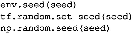
• To make sure that results are reproducible, we set the random number generator seeds (for the reinforcement learning environment, TensorFlow, and NumPy):

  

• We remove the plots from the tutorial code, as these are not particularly useful during automated tuning.

• Finally, we return the variable avg_reward_list, which is the average reward of the last 40 episodes. This returned value will be the objective function value that our tuner Sequential Parameter Optimization Toolbox (SPOT) observes.

• Note that all reward values we consider will be negated, since most of the procedures we employ assume smaller values to be better.

More details on the tuned parameters are given next.

3.2 Tuned Parameters

In the previous Sect. 11.3.1, we already briefly introduced the tuned parameters and their default values: num_hidden=256, critic_lr=0.002, actor_lr=0.001, gamma=0.99, tau=0.005, activation=“relu”. Some of these we may recognize, matching parameters of neural networks that we considered throughout other parts of this book: num_hidden corresponds to the previously discussed $\texttt {units}$, but is a scalar value (it is reused to define the size of all the larger layers in all networks). Instead of a single $\texttt {learning\_rate}$, we have separate learning rates for the actor and critic networks, critic_lr, and actor_lr.

The parameter gamma is new, as it is specific to actor-critic learning algorithms: it represents a discount factor which is applied to estimated rewards as a multiplicator. The parameter tau is also new, representing a multiplicator that is used when updating the weights of the target networks. Finally, $\texttt {activation}$ is the activation function (here: shared between all internal layers). The parameters and their bounds are summarized in Table 11.1.

Table 11.1 The hyperparameters for our reinforcement learning example. Note that the defaults and bounds concern the actual scale of each parameter (not transformed). Defaults denote the values from the original Keras tutorial, not the formal defaults from the Keras function interfaces

List of configurations

The following code snippet shows the code used to define this parameter search space for SPOT in R.

Note that we set a single fixed parameter, max_episodes, limiting the evaluation of the learning process to 50 episodes.

3.3 Further Configuration of SPOT

SPOT is configured to use 300 evaluations, which are spent as follows: Each evaluation is replicated (evaluated repeatedly) five times, to account for noise. Noise is a substantial issue in reinforcement learning cases like this one.

30 different configurations are tested in the initial design, leading to 150 evaluations (including the replications). The remaining 150 evaluations are spent by the iterative search procedure of SPOT. Due to replications, this implies that 30 further configurations are tested. Also, due to the stochastic nature of the problem, we set the parameter noise=TRUE.

The employed surrogate model is Kriging (a.k.a. Gaussian process regression), which is configured to use the so-called nugget effect (useLambda=TRUE), but no re-interpolation (reinterpolate=FALSE).

In each iteration after the initial design, a Differential Evolution algorithm is used to search the surrogate model for a new, promising candidate. The Differential Evolution algorithm is allowed to spend 2400 evaluations of the surrogate model in each iteration of SPOT.

For the sake of reproducibility, random number generator seeds are specified (seedSPOT, seedFun). Each replication will work with a different random number generator seed (iterated, starting from seedFun).

Arguments for calling SPOT

The respective configuration and function call is

3.4 Post-processing and Validating the Results

To determine how well the tuning worked, we perform a short validation experiment at the end. There, we spend 10 replications to evaluate the best found solution. We also spend more episodes for this test (i.e., max_episodes=100). This provides a less noisy and more reliable estimate of our solution’s performance, compared to the respective performance of the default settings from the tutorial (see Table 11.1).

Note that this step requires a bit of data processing, where we first aggregate our result data set by computing mean objective values (i.e., over the 5 replications), to determine which configuration was evaluated to work best on average.

4 Results

Table 11.2 compares the parameters of the best solution found during tuning with those of the defaults from the tutorial. It also lists the respective performance (average reward) and its standard deviation. We can load the result file created after tuning to create a visual impression of this comparison (Fig. 11.2).

Table 11.2 The hyperparameter values of the best solution found during tuning, compared against those of the defaults from the Keras tutorial by Singh (2020). It also lists the respective performance (mean neg. reward) and its standard deviation. Mean and standard deviation are computed over 10 replications, evaluated with 100 episodes

Interestingly, much smaller size of the dense layers (num_hidden=64) seems to suffice for the tuned solution. The larger tutorial network uses 256 units. The tuned algorithm also uses a larger learning rate for the critic network, compared to the actor network. The parameters gamma and tau deviate strongly from the respective defaults.

Fig. 11.2

Boxplot comparing the default and tuned configurations of the reinforcement learning process, in terms of their negated reward

5 Severity: Validating the Results

Let us proceed to analyze the average negated reward attained between the tuned and default parameters using severity. The pre-experimental runs indicate that the difference is $\bar{x} =$ 13.76. Because this value is positive, we can assume that the tuned solution is superior. The standard deviation is $s_d =$ 32.67. Based on Eq. 5.14, and with $\alpha =$ 0.05, $\beta =$ 0.2, and $\Delta =$ 40, we can determine the number of runs for the full experiment.

For a relevant difference of 40, approximately 8 completing runs per algorithm are required. Hence, we can proceed directly to evaluate the severity as sufficient runs have already been performed.

The decision based on the p-value of 0.0915 is to not reject $H_0$. Considering a target relevant difference $\Delta$ $=$ 40, the severity of not rejecting $H_0$ is 0.99, and thus it strongly supports the decision of not rejecting the $H_0$. The corresponding severity plot is shown in Fig. 11.3. Analyzing the results of hypothesis testing and severity as shown in Table 11.3, the differences in terms of parameter values do not seem to manifest in the performance values. It can be observed in Table 11.2 that a comparatively minor difference in mean performance is observed, while the difference in standard deviation is a bit more pronounced. However, this cannot be deemed as statistically significant relevance.

Overall, this matches well with what we see from a more detailed look at the tuning results (Fig. 11.4):

Fig. 11.3

Reinforcement learning. Severity of not rejecting H0 (red), power (blue), and error (gray). Left: the observed mean $\bar{x} =$ 13.76 is smaller than the cut-off point $c_{1-\alpha } =$ 16.99. Right: Severity of not rejecting H0 as a function of $\Delta$

Table 11.3 Case Study IV: Result Analysis

Fig. 11.4

Parallel plot of the achieved performance values during tuning. Red lines denote poor configurations (poor performance), blue lines better configurations

6 Summary and Discussion

In summary, the investigation shows that large parts of the search space lead to poorly performing configurations of the algorithm. Still, there seems to be a broad spectrum of potentially well-performing configurations, which interestingly include fairly small networks (i.e., with few units). This observation may be linked to the complexity of the problem, which is a relatively simple reinforcement learning scenario with few states and actions.

The tuned solution seems to work a little better than the default settings from the tutorial (Singh 2020), but those defaults are still competitive. It is reasonable to assume that the tutorial defaults were chosen with care (potentially by some sort of tuning procedure, or relevant experience by the tutorial’s author) and are well-suited for this problem. While the smaller network implies faster computation, the larger network has the advantage of being more easily transferred to more complex reinforcement learning cases.