
Abstract
This chapter focuses on the AI development framework developed by Huawei—MindSpore. Firstly, it introduces the architecture of MindSpore and how it is designed. Next, it analyses the problems and difficulties of AI development frameworks. Lastly, it further presents the framework base on the development and application of MindSpore.
You have full access to this open access chapter, Download chapter PDF
This chapter focuses on the AI development framework developed by Huawei—MindSpore. Firstly, it introduces the architecture of MindSpore and how it is designed. Next, it analyses the problems and difficulties of AI development frameworks. Lastly, it further presents the framework base on the development and application of MindSpore.
5.1 Introduction to MindSpore Development Framework
MindSpore is a Huawei self-developed AI development framework which can achieve device-edge-cloud all-scenario on-demand collaboration. It provides a unified all-scenario API which enable end-to-end model development, execution and deployment.
MindSpore adopts a device-edge-cloud on-demand collaborative distributed architecture, a new paradigm of native differential programming, and a new AI Native execution mode to achieve higher resource efficiency, security and reliability, while lowering the entrance standards for AI development and giving a full play to the computing power of the Ascend AI processor to realize inclusive AI application.
5.1.1 MindSpore Architecture
The architecture of MindSpore consists of three parts: development, execution and deployment. As shown by Fig. 5.1, the processors that can be deployed include CPU, GPU and Ascend AI processors (Ascend310, Ascend910).

The architecture of MindSpore
The development is a unified all-scenario API (Python API) which provides users with a unified model training, inference, and export interface, as well as a unified data processing, enhancement, and format conversion interface.
The development includes functions such as graph high level optimization (GHLO), hardware-independent optimization (e.g., dead code elimination, etc.), automatic parallelism, and automatic differentiation. These functions also support the design concept of a unified all-scenario API.
MindSpore IR in execution has a native computational graph representation, and a unified intermediate representation (IR), based on which MindSpore performs the optimization on compiler pass.
The execution includes hardware-related optimization, parallel Pipeline execution layer, and deep optimization related to combination of software and hardware, such as operator fusion and buffer fusion. These features enable the automatic differentiation, automatic parallel, and automatic tuning.
The deployment adopts distributed architecture of the on-demand device-edge-cloud collaboration, with deployment, scheduling, and communication acting on the same layer, contributing to the all-scenario on-demand collaboration.
In a nutshell, MindSpore integrates the easy development (AI algorithm as code), efficient operation (supporting optimization of Ascend AI processor and GPU), and flexible deployment (all-scenario on-demand collaboration) together in one framework.
5.1.2 How Is MindSpore Designed
In response to the challenges faced by AI developers in the industry, such as high development entrance standards, high operating costs, and difficulties of deployment, MindSpore proposes three technological innovations correspondingly: new programming paradigm, new execution mode, and new collaboration mode to help the developers realize the development and deployment of AI applications in an easier and more efficient manner.
-
1.
New Programming Paradigm
The design concept of the new programming paradigm is proposed to deal with the challenges for the AI development.
The challenges for the development mainly include:
-
(a)
High skill requirements. Developers are required to have relevant theoretical knowledge and mathematical skills of AI, computer systems, software to get engaged in AI development, raising the bar of entrance.
-
(b)
Difficult black-box optimization. The un-interpretability and the “black-box” feature of AI algorithms make it more difficult to tune parameters.
-
(c)
Difficult parallel planning. Influenced by the technological progress, the volume of data is getting larger and larger, and the models are getting bigger and bigger, making parallel computing inevitable. Parallel planning relies heavily on the technicians’ personal experience, requiring technicians to not only be a professional of data and models but also be acquainted with the distributed systems architecture.
The AI algorithm in the new programming paradigm is code itself, which lowers the bar of AI development. The new AI programming paradigm based on the mathematical native expression allows algorithm experts to focus on AI innovation and exploration, as shown in Fig. 5.2.
-
(a)
Automatic Differentiation
Automatic differentiation (AD) is the soul of the deep learning framework. Generally speaking, AD refers to a method of automatically computing the derivative of a function. In machine learning, these derivatives can update the weights. In the natural science with a broader connotation, these derivatives can also be used in subsequent computations. The development of automatic differentiation is shown in Fig. 5.3.
During the development of automatic differentiation, there are three types of automatic differentiation techniques as follows.
-
Conversion based on static calculation graph: The network is converted into static calculation diagram at compile time, and then the chain rule is applied to the calculation diagram to realize automatic differentiation. For example, Tensorflow can optimize the network performance by static compilation technology. However, it is very complex to build or debug the network.
-
Conversion based on dynamic calculation graph: The operation track of the network during forward propagation is recorded by operator overloading, and then the chain rule is applied to the dynamically generated calculation graph to realize automatic differentiation. For example, PyTorch is very convenient to use, but it is difficult to optimize the performance to the ultimate level.
-
Conversion based on source code: Based on a functional programming framework, it adopts just-in-time (JIT) compilation to perform automatic differentiation transformation on the intermediate representation (a representation of a program during compilation). It also supports automatic differentiation of automatic control flow. So it is very convenient to build models, just as PyTorch. At the same time, MindSpore can do static compilation and optimization of neural networks, so its performance is also very good. The comparison of automatic differentiation technologies is shown in Table 5.1, and the comparison of performance and programmability is shown in Fig. 5.4.
The MindSpore automatic differentiation technology has the following advantages.
-
Programmability: Differentiability can be achieved by Python universal languages based on IR primitives (each primitive operation in MindSpore IR corresponds to the basic function in basic algebra).
-
Performance: Compiler optimization, operator reverse auto-tuning.
-
Debugging: Diversified visual interfaces and supports dynamic execution.
-
-
(b)
Automatic Parallel
The deep learning models today often need to be parallelized because of their huge size. Currently, the manual model parallelism is adopted, which requires design model segmentation and awareness of cluster topology, which is difficult to realize. And it is also uneasy to assure high performance by the manual parallelism, not to mention tuning.
MindSpore can automatically parallel the code written in serial, realize distributed parallel training automatically and keep high performance.
Generally speaking, parallel training can be divided into model parallel and data parallel. Data parallel is easier to understand, which means each sample can complete the forward propagation independently, and finally summarize the propagation results. In contrast, model parallel is more complicated, and we need to manually write all the parts that need to be paralleled with logic of “parallel thinking”.
MindSpore introduces a key innovation technology—automatic full-graph segmentation. As shown in Fig. 5.5, the full graph is segmented according to the operator input and output data, that is, each operator in the graph is divided into clusters and then complete the parallel operation. This technology combines data parallel and model parallel. Cluster topology is adopted to automatically schedule the execution of sub-graphs to minimize communication overhead.
The goal of MindSpore automatic parallel is to build a training method that combines data parallelism, model parallelism, and hybrid parallelism. It will automatically select a model segmentation method featuring the lowest cost to implement automatic distributed parallel training.
The operator fine-granularity method of MindSpore segmentation is very complicated. But developers do not need to take into account the underlying implementation, as long as they endow the top-level API with high efficiency of calculations.
Generally speaking, the new programming paradigm not only realizes the “AI algorithm as code”, lowering the threshold of AI development, but also enables efficient development and debugging. For example, it can efficiently complete automatic differentiation, realize the automatic parallel of one line of code, and complete debugging and running of one line of code.
Transformer, a classic algorithm used by developers to implement natural language processing, is made real by the MindSpore framework. During the development and debugging process, both dynamic and static implementation combined, and the debugging is transparent and simple. From the final structure, the amount of code on the MindSpore framework is 2000, which, compared with 2500 lines of Tensorflow, is about 20% less, but with efficiency improved more than 50%.
-
(a)
-
2.
New Execution Mode
The design concept of the new execution mode is proposed in response to the challenges of the execution.
The challenges posed to the execution are as follows:
-
(a)
The complexity of AI computation and the diversity of computing power: various types of computing powers, such as CPU core, cube unit, vector unit; computation of scalar quantity, vector quantity, and tensor quantity; mixed precision computation; dense matrix and sparse matrix computation.
-
(b)
In the case of multi-GPU operation, as the number of nodes increases, the performance is difficult to increase linearly, resulting in high parallel control overhead.
The new execution mode adopts Ascend Native execution engine of and proposes on-device execution, as shown in Fig. 5.6. The full graph offload execution and the depth map optimization are utilized, giving full play to the strong computing power of Ascend AI processor.
There are two technical cores of On-Device implementation, as follows.
-
(a)
Full graph sink execution, giving full play to the strong computing power of the Ascend AI processor. This technique addresses the challenges faced by model execution under super chip computing power, such as memory wall, high interaction overhead, difficulty in data supply, etc. Execution is partly done on the host and partly on terminal devices, which leads to much higher overhead of interaction than the overhead of execution, resulting in a low accelerator occupancy rate. MindSpore, adopting chip-oriented depth map optimization technology, minimizes synchronization waiting and maximizes the parallel degree of data-calculation-communication synergy, sinking the entire data+ full graph calculation to the Ascend AI processor, thus offering the best and optimal result. The final result is a 10 times improvement in training performance compared to the graph scheduling method on the host side.
-
(b)
Data-driven large-scale distributed gradient aggregation. This technology addresses the challenges of distributed gradient aggregation under super chip computing power, i.e., the synchronization overhead of central control and the communication overhead of frequent synchronization in a single iteration of ResNet-50 in 20 ms. The traditional method requires three synchronization steps to complete AllReduce and the data-driven autonomous AllReduce without control overhead.
MindSpore achieves a decentralized autonomous AllReduce algorithm through adaptive graph segmentation optimization driven by gradient data, so as to keep gradient aggregation in the same step and the parallel of computation and communications, as shown in Fig. 5.7.
Figure 5.8 shows an example in computer vision. Neural network ResNet-50 V1.5 is adopted to carry out training on the ImageNet 2012 dataset based on their best batch size respectively. It can be seen that the speed of MindSpore framework on Ascend 910 is much higher than that on other frameworks and other mainstream training cards.
-
(a)
-
3.
New Collaborative Model
The design concept of the new collaboration model is proposed in response to the challenges of the deployment.
The challenges to the deployment are as follows.
-
(a)
Device, edge, and cloud application scenarios have different requirements, goals and constraints. For instance, the devide of mobile phone may prefer a lighter model, while the cloud may require higher precision.
-
(b)
Different hardware has different accuracy and speed, as shown in Fig. 5.9.
-
(c)
The diversity of hardware architectures leads to deployment differences and performance uncertainties in all scenarios, and the separation of training and inference leads to model isolation.
In the new collaboration mode, all scenarios can be coordinated on-demand, resulting in better resource efficiency and privacy protection, security and credibility, and supporting one-time development and multiple deployments. The models can be big or small and can be deployed flexibly, offering a consistent development experience.
MindSpore has the following three key technologies regarding the new collaborative model.
-
(a)
The unified model IR can cope with differences in different language scenarios, compatible with customized data structure, bringing a consistent deployment experience.
-
(b)
The hardware of the framework is also developed by Huawei, and the software-hardware collaborative graph optimization technology can shield the scene differences.
-
(c)
The device-cloud collaborative federated meta learning strategy breaks the boundary between the device and cloud, realizing real-time update of the multi-device collaborative model.
The final effect of these three key technologies is under a unified architecture, the deployment performance of the all-scenario model is consistent, and the accuracy of the personalized model is significantly improved, as shown in Fig. 5.10.
The vision and value of MindSpore is to provide an AI computing platform of efficient development, excellent performance, and flexible deployment, to lower the entrance bar for AI development, release the computing power of the Ascend AI processor, and realize inclusive AI, as shown in Fig. 5.11.
-
(a)

New programming paradigm of MindSpore

The development of automatic differentiation

Comparison of automatic differentiation performance and programmability

Automatic full-graph segmentation

On-device execution

Decentralized autonomous AllReduce algorithm

Comparison between MindSpore and TensorFlow

Challenges of the deployment

On-demand collaboration and consistent development

Vision and value of MindSpore
5.1.3 Advantages of MindSpore
MindSpore has the following advantages.
-
1.
User-Friendliness in Development
-
(a)
Automatic differentiation, unified programming of network and operator, native expression of functional formulas and algorithms, and automatic generation of reverse network operators.
-
(b)
Automatic parallelism, optimal efficiency model parallelism achieved by automatic model segmentation.
-
(c)
Automatic tuning, the same set of codes for dynamic graph and static graph.
-
(a)
-
2.
High Efficiency in execution
-
(a)
On-device execution, giving full play to the strong computing power of Ascend AI processor.
-
(b)
Pipeline optimization, maximizing parallel performance.
-
(c)
Depth map optimization, computing power and precision of adaptive AI Core (Da Vinci architecture, check Chap. 6 for details).
-
(a)
-
3.
Flexibility in Deployment
-
(a)
On-demand collaborative computing of device, edge and cloud to better protect privacy.
-
(b)
The unified architecture of device, edge and cloud enables one-time development and deployment on demand.
-
(a)
-
4.
Equivalent to Industrial Open-Source Frameworks
MindSpore ranks abreast with the industry’s open source frameworks, supporting CPU, GPU and other hardware, with the self-developed chips and cloud services prioritized in services.
-
5.
Upward
MindSpore is enabled to dock with third-party frameworks. It can connect with third-party frameworks through Graph IR (training front-end docking, inference model docking), and developers can extend.
-
6.
Downward
MindSpore can interface with third-party chips to help developers expand MindSpore’s application scenarios and prosper the AI ecosystem.
5.2 MindSpore Development and Application
5.2.1 Environment Setup
Setting up the MindSpore development environment requires the installation of Python version 3.7.5 or above. MindSpore supports hardware platforms such as CPU, GPU, and Ascend910, and supports operating systems such as Ubuntu. It can be installed directly with the installation package or compiled source code, as shown in Fig. 5.12.

Installation of MindSpore
Now take the installation in an Ubuntu 18.04 system with CPU environment as an example to introduce the installation steps. The requirements of MindSpore CPU version on system and software are shown in Table 5.2.
GCC 7.3.0 can be installed directly through the apt command.
If Python is already installed, make sure to add Python to the system variable. You can also use the command “Python-Version” to check whether the version of Python meets the requirements.
-
1.
Installation by Pip
Use the following pip command to install MindSpore.
pip install –y MindSpore-cpu
Please add pip to the system variable to ensure that Python-related toolkits can be installed directly through pip. If pip is not installed in the current system, you can download from the official website and install it. Requirements.txt contents are shown in Fig. 5.13.
When the Internet is connected, reliance items will be automatically downloaded during whl package installation. In other cases, you need to manually install reliance items.
-
2.
Installation by Source Code Compilation
The procedures to install MindSpore by source code are as follows.
-
(a)
Source code for downloading source code from code repository are as follows:
-
(b)
Run the following command in the root directory of the source code to compile MindSpore:
-
Before executing the above commands, make sure that the path where the executable file cmake and path store has been added to the environment variable PATH.
-
Confirm that the git tool is installed. Then the command “git clone” will be executed in build.sh to obtain the code of the third-party code repository.
-
If the compiler performance is strong, you can add -j{Number of threads} in to script to increase the number of threads. For example, bash build.sh -e cpu -j12.
-
-
(c)
Execute the following command to install MindSpore.
chmod +x build/package/MindSpore-{version}-cp37-cp37m-linux_{arch}.whl pip install build/package/MindSpore-{version}-cp37-cp37m-linux_{arch}.whl
-
(d)
Execute the following command. If the output is “No module named ‘mindspore’”, it means that the installation was not successful.
python -c 'import MindSpore'
Fig. 5.13 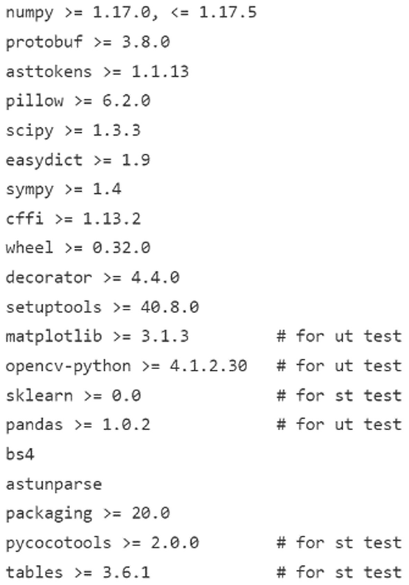
Contents of requirements.txt
-
(a)

5.2.2 Components and Concepts Related to MindSpore
-
1.
Component
Some commonly used components and descriptions by MindSpore are shown in Table 5.3.
In MindSpore, the most basic data structure is also the tensor. There are several common tensor operations as follows:
asnumpy() size() dim() dtype() set_dtype() tensor_add(other: Tensor) tensor_mul(ohter: Tensor) shape() __str__# convert into string
These tensor operations can basically be understood by reading their names, such as asnumpy() means conversion to NumPy array, tensor_add() means tensor addition.
-
2.
Programming Concept: Operation
There are several common operations in MindSpore as follows.
-
(a)
Array: Array-related operators as follows:
-ExpandDims - Squeeze -Concat - OnesLike -Select - StridedSlice -ScatterNd ...
-
(b)
Math: mathematical calculations related operators as follows:
-AddN - Cos -Sub - Sin -Mul - LogicalAnd -MatMul - LogicalNot -RealDiv - Less -ReduceMean - Greater ...
-
(c)
Nn: Network operators as follows:
-Conv2D - MaxPool -Flatten - AvgPool -Softmax - TopK -ReLU - SoftmaxCrossEntropy -Sigmoid - SmoothL1Loss -Pooling - SGD -BatchNorm - SigmoidCrossEntropy ...
-
(d)
Control: control operators as follows:
ControlDepend
-
(a)
-
3.
Programming Concept: Cell
-
(a)
Cell defines the basic modules for performing calculations. Cell objects can be executed directly.
-
__init__, initialize parameters (parameter), sub-module (cell), operator (primitive) and other components, and perform initialization verification.
-
Construct, which defines the execution process. In graph mode, it will be compiled into graphs for execution. There are some grammatical restrictions.
-
Bprop (optional), the reverse of the custom module. When this function is not defined, automatic differentiation will be used to calculate the reverse of the construct part.
-
-
(b)
The predefined cells in MindSpore mainly include: commonly used loss functions (such as SoftmaxCrossEntropyWithLogits, MSELoss), commonly used optimizers (such as Momentum, SGD, Adam), and commonly used network packaging functions (such as TrainOneStepCell, WithGradCell).
-
(a)
-
4.
Programming Concept: MindSporeIR
-
(a)
MindSporeIR is a concise, efficient, and flexible graph-based functional IR that can express functional semantics such as free variables, higher-order functions and recursion.
-
(b)
Each graph represents a function definition, and the graph consists of ParameterNode, ValueNode, and ComplexNode (CNode).
-
(a)
5.2.3 Realization of Handwritten Digit Recognition with Mindspore
-
1.
Overview
This tutorial uses a simple image classification example to demonstrate the basic functions of MindSpore. For general users, it takes 20–30 min to complete the entire sample practice. This is a simple and basic application process, and other advanced and complex applications can be extended based on this basic process.
This sample will implement a simple image classification, and the overall process is as follows:
-
(a)
Process the needed dataset. The MNIST dataset is used in this example.
-
(b)
Define a network. The LeNet network is used in this example.
-
(c)
Define the loss function and optimizer.
-
(d)
Load the dataset and perform training. After the training is complete, check the result and save the model file.
-
(e)
Load the saved model for inference.
-
(f)
Validate the model, load the test dataset and trained model, and validate the result accuracy.
-
(a)
-
2.
Preparation
Before the practice, check whether MindSpore has been correctly installed. If not, install MindSpore on your computer by referring to Sect. 5.2.1. In addition, you shall have basic mathematical knowledge such as Python programming basics, probability, and matrix.
Next, let’s embark on the journey of MindSpore.
-
(a)
Download the MNIST Dataset.
The MNIST dataset used in this example consists of 10 classes of 28 × 28 pixels grayscale images. It has a training set of 60,000 examples, and a test set of 10,000 examples.
The download page of the MNIST provides four download links of dataset files. The first two links are required for data training, and the last two links are required for data test.
Download the files, decompress them, and store them in the workspace directory: ./MNIST_Data/train and ./MNIST_Data/test.
The directory structure is as follows:
└─MNIST_Data ├─test │ t10k-images.idx3-ubyte │ t10k-labels.idx1-ubyte └─train train-images.idx3-ubyte train-labels.idx1-ubyte
To facilitate the operation, we add the function of automatically downloading datasets in the sample script code.
-
(b)
Import Python Libraries and Modules
Before the usage, import Python libraries.
Now the libraries are used. For better understanding, other required libraries will be introduced when we use them in practices.
import os
-
(c)
Configure the Running Information
Before officially compiling the code, we need to know the basic information about the hardware and backend required for MindSpore at run-time.
We can use context.set_context to configure the information required at run-time, such as the running mode, backend information, and hardware information.
Import the context module and configure the required information. The codes are exemplified as follows.
import argparse from MindSpore import context if __name__ == "__main__": parser = argparse.ArgumentParser(description='MindSpore LeNet Example') parser.add_argument('--device_target', type=str, default="Ascend", choices=['Ascend', 'GPU', 'CPU'], help='device where the code will be implemented (default: Ascend)') args = parser.parse_args() context.set_context(mode=context.GRAPH_MODE, device_target=args.device_target, enable_ mem_reuse=False) ...
We use graph mode when deploy the above-mentioned example. You can configure hardware information according to the site requirements. For instance, if the code runs on the Ascend AI processor, then device_target chooses Ascend. This rule also applies to the code running on the CPU and GPU. For details about parameters, see context.set_context () interface for more details.
-
(a)
-
3.
Processing Data
Datasets are important for training. A good dataset can effectively improve training accuracy and efficiency. Generally speaking, before loading a dataset, you need to perform some operations on the dataset.
Define the create_dataset() function to create a dataset. In this function, we need to define the data augmentation and processes to be performed.
-
(a)
Define the dataset.
-
(b)
Define parameters required for data augmentation and processing.
-
(c)
Generate corresponding data augmentation according to the parameters.
-
(d)
Use the map() mapping function to apply data processes to the dataset.
-
(e)
Process the generated dataset.
The sample codes for processing the dataset are as follows:
import MindSpore.dataset as ds import MindSpore.dataset.transforms.c_transforms as C import MindSpore.dataset.transforms.vision.c_transforms as CV from MindSpore.dataset.transforms.vision import Inter from MindSpore.common import dtype as mstype def create_dataset(data_path, batch_size=32, repeat_size=1, num_parallel_workers=1): """ create dataset for train or test Args: data_path: Data path batch_size: The number of data records in each group repeat_size: The number of replicated data records num_parallel_workers: The number of parallel workers """ # define dataset mnist_ds = ds.MnistDataset(data_path) # define operation parameters resize_height, resize_width = 32, 32 rescale = 1.0 / 255.0 shift = 0.0 rescale_nml = 1 / 0.3081 shift_nml = -1 * 0.1307 / 0.3081 # define map operations resize_op = CV.Resize((resize_height, resize_width), interpolation=Inter.LINEAR) # resize images to (32, 32) rescale_nml_op = CV.Rescale(rescale_nml, shift_nml) # normalize images rescale_op = CV.Rescale(rescale, shift) # rescale images hwc2chw_op = CV.HWC2CHW() # change shape from (height, width, channel) to (channel, height, width) to fit network. type_cast_op = C.TypeCast(mstype.int32) # change data type of label to int32 to fit network # apply map operations on images mnist_ds = mnist_ds.map(input_columns="label", operations=type_cast_op, num_parallel_ workers=num_parallel_workers) mnist_ds = mnist_ds.map(input_columns="image", operations=resize_op, num_parallel_ workers=num_parallel_workers) mnist_ds = mnist_ds.map(input_columns="image", operations=rescale_op, num_parallel_ workers=num_parallel_workers) mnist_ds = mnist_ds.map(input_columns="image", operations=rescale_nml_op, num_parallel_ workers=num_parallel_workers) mnist_ds = mnist_ds.map(input_columns="image", operations=hwc2chw_op, num_parallel_ workers=num_parallel_workers) # apply DatasetOps buffer_size = 10000 mnist_ds = mnist_ds.shuffle(buffer_size=buffer_size) # 10000 as in LeNet train script mnist_ds = mnist_ds.batch(batch_size, drop_remainder=True) mnist_ds = mnist_ds.repeat(repeat_size) return mnist_ds
The notes for the codes are as follows.
Batch_size: the amount of data in each group. Currently, each group contains 32 data records.
Repeat_size: the number of replicated datasets.
Firstly, implement the shuffle and batch operations, and then perform the repeat operation to ensure that data is nonrepetitive during one epoch.
MindSpore supports multiple data processing and augmentation operations, which are usually used in combination.
-
(a)
-
4.
Defining the Network
Here we choose the relatively simple LeNet network. In addition to the input layer, the LeNet network has seven layers, including two convolutional layers, two down-sampling layers (pooling layers), and three full-connected layers. Each layer contains different numbers of training parameters, as shown in Fig. 5.14:
We need to initialize the full-connected layers and convolutional layers.
Mindspore supports multiple parameter initialization methods, such as TruncatedNormal, Normal, and Uniform. For details, see the illustration in the Mindspore.common.initializer module of the MindSpore API. This case uses the parameter initialization method TruncatedNormal.
Following are the sample codes exemplified for initializing the full-connected layers and convolutional layers:
import MindSpore.nn as nn from MindSpore.common.initializer import TruncatedNormal def weight_variable(): """ weight initial """ return TruncatedNormal(0.02) def conv(in_channels, out_channels, kernel_size, stride=1, padding=0): """ conv layer weight initial """ weight = weight_variable() return nn.Conv2d(in_channels, out_channels, _size=kernel_size, stride=stride, padding= padding weight_init=weight, has_bias=False, pad_mode="valid") def fc_with_initialize(input_channels, out_channels): """ fc layer weight initial """ weight = weight_variable() bias = weight_variable() return nn.Dense(input_channels, out_channels, weight, bias)
To use MindSpore to define the neural network, inheriting MindSpore.nn.Cell is required. Cell is the base class of all neural networks (such as Conv2d).
Each layer of a neural network will need to be defined by the __init__ () method in advance, and then define the construct() method to complete the forward construction of the neural network. According to the structure of the LeNet network, define the network layers as follows:
-
5.
Defining the Loss Function and Optimizer
-
(a)
The concept of loss function and optimizer.
Loss function: Also known as objective function, loss function is used to measure the differences between the predicted value and the actual value. Deep learning reduces the value of the loss function by iteration. Defining a good loss function can effectively improve the model performance.
Optimizer: It is used to minimize the loss function so as to optimize the model during training.
After the loss function is defined, the weight-related gradient of the loss function can also be obtained. The gradient is used to indicate the weight optimization direction for the optimizer and improve the model performance.
-
(b)
Defining the Loss Function
The loss functions supported by MindSpore include SoftmaxCrossEntropyWithLogits, L1Loss, MSELoss. The loss function SoftmaxCrossEntropyWithLogits is used in the following sample codes:
class LeNet5(nn.Cell): """ Lenet network structure """ #define the operator required def __init__(self): super(LeNet5, self).__init__() self.batch_size = 32 self.conv1 = conv(1, 6, 5) self.conv2 = conv(6, 16, 5) self.fc1 = fc_with_initialize(16 * 5 * 5, 120) self.fc2 = fc_with_initialize(120, 84) self.fc3 = fc_with_initialize(84, 10) self.relu = nn.ReLU() self.max_pool2d = nn.MaxPool2d(kernel_size=2, stride=2) self.flatten = nn.Flatten() #use the preceding operators to construct networks def construct(self, x): x = self.conv1(x) x = self.relu(x) x = self.max_pool2d(x) x = self.conv2(x) x = self.relu(x) x = self.max_pool2d(x) x = self.flatten(x) x = self.fc1(x) x = self.relu(x) x = self.fc2(x) x = self.relu(x) x = self.fc3(x) return x from MindSpore.nn.loss import SoftmaxCrossEntropyWithLogits
Call the defined loss funciton in __main__ function. The sample codes are as follows.
if __name__ == "__main__": ... #define the loss function net_loss = SoftmaxCrossEntropyWithLogits(is_grad=False, sparse=True, reduction='mean') ...
-
(c)
Defining the Optimizer
The optimizers supported by MindSpore include Adam, AdamWeightDecay and Momentum. The following sample codes are based on the Momentum optimizer, which is quite popular:
if __name__ == "__main__": ... #learning rate setting lr = 0.01 momentum = 0.9 #create the network network = LeNet5() #define the optimizer net_opt = nn.Momentum(network.trainable_params(), lr, momentum) ...
-
(a)
-
6.
Training the Network
-
(a)
Save the Configured Model
MindSpore provides the callback mechanism to execute customized logic during training. Here we list ModelCheckpoint and LossMonitor provided by the framework as examples.
from MindSpore.train.callback import ModelCheckpoint, CheckpointConfig if __name__ == "__main__": ... # set parameters of check point config_ck = CheckpointConfig(save_checkpoint_steps=1875, keep_checkpoint_max=10) # apply parameters of check point ckpoint_cb = ModelCheckpoint(prefix="checkpoint_lenet", config=config_ck) ...
ModelCheckpoint can save network models and parameters for subsequent fine-tuning. And LossMonitor can monitor the changes of the loss value during training.
-
(b)
Configure the Network Training
Through the model.train() API provided by MindSpore we can easily train the network. Here, we set epoch-size as 1 to train the dataset for 1 iteration.
from MindSpore.nn.metrics import Accuracy from MindSpore.train.callback import LossMonitor from MindSpore.train import Model ... def train_net(args, model, epoch_size, mnist_path, repeat_size, ckpoint_cb): """define the training method""" print("============== Starting Training ==============") #load training dataset ds_train = create_dataset(os.path.join(mnist_path, "train"), 32, repeat_size) model.train(epoch_size, ds_train, callbacks=[ckpoint_cb, LossMonitor()], dataset_ sink_mode=False) ... if __name__ == "__main__": ... epoch_size = 1 mnist_path = "./MNIST_Data" repeat_size = epoch_size model = Model(network, net_loss, net_opt, metrics={"Accuracy": Accuracy()}) train_net(args, model, epoch_size, mnist_path, repeat_size, ckpoint_cb) ...
Here in the train_net() method, we load the training dataset we downloaded before, and mnist_path is the MNIST dataset path.
-
(a)
-
7.
Run and View the Result
Run the script code using the following command:
python lenet.py --device_target=CPU
Explanation is as follows.
lenet.py: the script file you wrote.
--device_target CPU: Specify the hardware platform. The parameters are ‘CPU’, ‘GPU’ or ‘Ascend’.
Loss values are printed during training, as shown in the following figure. Although loss values may fluctuate, they would gradually decrease. Loss values for every running may be different because of their randomicity. The following is an example of loss values output during training.
epoch: 1 step: 262, loss is 1.9212162 epoch: 1 step: 263, loss is 1.8498616 epoch: 1 step: 264, loss is 1.7990671 epoch: 1 step: 265, loss is 1.9492403 epoch: 1 step: 266, loss is 2.0305142 epoch: 1 step: 267, loss is 2.0657792 epoch: 1 step: 268, loss is 1.9582214 epoch: 1 step: 269, loss is 0.9459006 epoch: 1 step: 270, loss is 0.8167224 epoch: 1 step: 271, loss is 0.7432692 ...
The following is an example of model files saved after training, namely saving the model parameter files:
checkpoint_lenet-1_1875.ckpt
Explanation is as follows.
checkpoint_lenet-1_1875.ckpt: It refers to the saved model parameter file. The checkpoint_network means the name of network, epoch No. means the serial number of epoch, and .ckpt means the serial number of the step.
-
8.
Validate the Model
After obtaining the model file, we verify the generalization ability of the model.
Use the model.eval() interface to load testing dataset.
Inference by using the saved model after training.
The sample codes are as follows:
from MindSpore.train.serialization import load_checkpoint, load_param_into_net ... def test_net(args,network,model,mnist_path): """define the evaluation method""" print("============== Starting Testing ==============") #load the saved model for evaluation param_dict = load_checkpoint("checkpoint_lenet-1_1875.ckpt") #load parameter to the network load_param_into_net(network, param_dict) #load testing dataset ds_eval = create_dataset(os.path.join(mnist_path, "test")) acc = model.eval(ds_eval, dataset_sink_mode=False) print("=========== Accuracy:{}=========".format(acc)) if __name__ == "__main__": ... test_net(args, network, model, mnist_path)
Explanation is as follows.
load_checkpoint(): This interface is used to load the CheckPoint model parameter file and return a parameter dictionary.
checkpoint_lenet-1_1875.ckpt: name of the saved CheckPoint model file.
load_param_into_net(): This interface is used to load parameters to the network.
Run the script code with the following command:
python lenet.py --device_target=CPU
An example of the result of running the verification model sample code is presented as follows:
============== Starting Testing ============== ========== Accuracy:{'Accuracy':0.9742588141025641} ===========
Here we can find that model accuracy is displayed in the output content. In the example, the accuracy reaches 97.4%, which indicates that the model quality is satisfactory.

LeNet-5 architecture
5.3 Chapter Summary
This chapter mainly introduces the deep learning framework MindSpore independently developed by Huawei. It firstly presents the three technological innovation of MindSpore in design, namely, the new execution mode, new collaboration mode, and the advantages such as friendly development, efficient execution, and flexible deployment. At last the chapter briefs about the development and application of MindSpore, and uses an example of image classification to illustrate the development procedure of MindSpore.
As MindSpore is still undergoing a rapid version iteration, please refer to the latest official materials to learn the specific operations.
5.4 Exercises
-
1.
MindSpore is an on-demand collaborative AI computing framework for all device-edge-cloud scenarios developed by Huawei. It provides a unified API for all scenarios, and provides device-to-device capability for model development, model operation and model deployment of all-scenario AI. What are the main features of the MindSpore architecture?
-
2.
To tackle the challenges faced by AI developers including high entrance standards, high costs of operation and difficult deployment, MindSpore proposes three technological innovations so as to achieve easier and more efficient development and deployment of AI application. What are them?
-
3.
The challenges of execution mode under super chip computing power: memory wall problem, high interaction overhead, difficult data supply, and the low occupancy rate of accelerator caused by the fact that the interaction overheads even surpasses the execution overhead as part of the operation is executed on host and part on device. What is the countermeasure offered by MindSpore?
-
4.
Use MindSpore to perform MNIST handwritten digit recognition.
Author information
Authors and Affiliations
Consortia
Rights and permissions
Open Access This chapter is licensed under the terms of the Creative Commons Attribution-NonCommercial-NoDerivatives 4.0 International License (http://creativecommons.org/licenses/by-nc-nd/4.0/), which permits any noncommercial use, sharing, distribution and reproduction in any medium or format, as long as you give appropriate credit to the original author(s) and the source, provide a link to the Creative Commons license and indicate if you modified the licensed material. You do not have permission under this license to share adapted material derived from this chapter or parts of it.
The images or other third party material in this chapter are included in the chapter's Creative Commons license, unless indicated otherwise in a credit line to the material. If material is not included in the chapter's Creative Commons license and your intended use is not permitted by statutory regulation or exceeds the permitted use, you will need to obtain permission directly from the copyright holder.
Copyright information
© 2023 The Author(s)
About this chapter

Cite this chapter
Huawei Technologies Co., Ltd.. (2023). Huawei MindSpore AI Development Framework. In: Artificial Intelligence Technology. Springer, Singapore. https://doi.org/10.1007/978-981-19-2879-6_5
Download citation
DOI: https://doi.org/10.1007/978-981-19-2879-6_5
Published:
Publisher Name: Springer, Singapore
Print ISBN: 978-981-19-2878-9
Online ISBN: 978-981-19-2879-6
eBook Packages: Computer ScienceComputer Science (R0)