Graphical Models

Abstract

In this chapter, we examine the problem of estimating the structure of the graphical model from observations. In the graphical model, each vertex is regarded as a variable, and edges express the dependency between them (conditional independence ). In particular, assume a so-called sparse situation where the number of vertices is larger than the number of variables.

Appendices

Appendix: Proof of Propositions

Proposition 15

(Lauritzen, 1996 [18])

$$\Theta _{AB}=\Theta ^T_{BA}=0 \ \Longrightarrow \ \det \Sigma _{A\cup C}\det \Sigma _{B\cup C}=\det \Sigma _{A\cup B\cup C}\det \Sigma _{C}$$

Proof: Applying Proof   $a=\left[ \begin{array}{c@{\quad }c} \Theta _{AA}&{}\Theta _{AC}\\ \Theta _{CA}&{}\Theta _{CC}\\ \end{array} \right]$, $b= \left[ \begin{array}{c} 0\\ \Theta _{CB}\\ \end{array} \right]$, $c= \left[ \begin{array}{c@{\quad }c} 0&\Theta _{BC} \end{array} \right]$, $d=\Theta _{BB}$,

$$\begin{aligned} e&=a-bd^{-1}c=\left[ \begin{array}{c@{\quad }c} \Theta _{AA}&{}\Theta _{AC}\\ \Theta _{CA}&{}\Theta _{CC}\\ \end{array} \right] - \left[ \begin{array}{c} 0\\ \Theta _{CB}\\ \end{array} \right] \Theta _{BB}^{-1} \left[ \begin{array}{c@{\quad }c} 0&\Theta _{BC} \end{array} \right] \\ {}&= \left[ \begin{array}{c@{\quad }c} \Theta _{AA}&{}\Theta _{AC}\\ \Theta _{CA}&{}\Theta _{CC}-\Theta _{CB}(\Theta _{BB})^{-1}\Theta _{BC}\\ \end{array} \right] \ ,\ \end{aligned}$$

in

$$\begin{aligned} \left[ \begin{array}{c@{\quad }c} a&{}b\\ c&{}d \end{array} \right] ^{-1}= \left[ \begin{array}{c@{\quad }c} e^{-1}&{}-e^{-1}bd^{-1}\\ -ed^{-1}c&{}d^{-1}+d^{-1}ce^{-1}bd^{-1} \end{array} \right] \ , \end{aligned}$$

(5.24)

we have

$$\begin{aligned} \left[ \begin{array}{c@{\quad }c} \Sigma _{A\cup C}&{}*\\ *&{}* \end{array} \right]&= \Theta ^{-1}= \left[ \begin{array}{c@{\quad }c@{\quad }c} \Theta _{AA}&{}\Theta _{AC}&{}0\\ \Theta _{CA}&{}\Theta _{CC}&{}\Theta _{CB}\\ 0&{}\Theta _{BC}&{}\Theta _{BB}\\ \end{array} \right] ^{-1}\\&= \left[ \begin{array}{c@{\quad }c} \left[ \begin{array}{c@{\quad }c} \Theta _{AA}&{}\Theta _{AC}\\ \Theta _{CA}&{}\Theta _{CC}-\Theta _{CB}(\Theta _{BB})^{-1}\Theta _{BC}\\ \end{array} \right] ^{-1} &{}*\\ *&{}* \end{array} \right] \ , \end{aligned}$$

which means

$$\begin{aligned} (\Sigma _{A\cup C})^{-1}= \left[ \begin{array}{c@{\quad }c} \Theta _{AA}&{}\Theta _{AC}\\ \Theta _{CA}&{}\Theta _{CC}-\Theta _{CB}(\Theta _{BB})^{-1}\Theta _{BC}\\ \end{array} \right] \ , \end{aligned}$$

(5.25)

where (5.24) is due to

$$\begin{aligned}&\left[ \begin{array}{c@{\quad }c} a&{}b\\ c&{}d \end{array} \right] \left[ \begin{array}{c@{\quad }c} e^{-1}&{}-e^{-1}bd^{-1}\\ -d^{-1}ce^{-1}&{}d^{-1}(I+ce^{-1}bd^{-1}) \end{array} \right] \\&= \left[ \begin{array}{c@{\quad }c} ae^{-1}-bd^{-1}ce^{-1}&{}-ae^{-1}bd^{-1}+bd^{-1}(I+ce^{-1}bd^{-1})\\ ce^{-1}-ce^{-1}&{}-ce^{-1}bd^{-1}+I+ce^{-1}bd^{-1} \end{array} \right] = \left[ \begin{array}{c@{\quad }c} I&{}0\\ 0&{}I \end{array} \right] \ . \end{aligned}$$

Similarly, we have

$$\begin{aligned} (\Sigma _C)^{-1}&= \Theta _{CC}- \left[ \begin{array}{c@{\quad }c} \Theta _{CA}&\Theta _{CB} \end{array} \right] \left[ \begin{array}{c@{\quad }c} \Theta _{AA}&{}0\\ 0&{}\Theta _{BB}\\ \end{array} \right] ^{-1} \left[ \begin{array}{c} \Theta _{AC}\\ \Theta _{BC}\\ \end{array} \right] \nonumber \\&=\Theta _{CC}-\Theta _{CA}(\Theta _{AA})^{-1}\Theta _{AC}-\Theta _{CB}(\Theta _{BB})^{-1}\Theta _{BC} \ . \end{aligned}$$

Thus, we have

$$\begin{aligned} \det \left[ \begin{array}{c@{\quad }c} I&{}(\Theta _{AA})^{-1}\Theta _{AC}\\ \Theta _{CA}&{}\Theta _{CC}-\Theta _{CB}(\Theta _{BB})^{-1}\Theta _{BC}\\ \end{array} \right] =\det (\Sigma _C)^{-1}\ . \end{aligned}$$

(5.26)

Furthermore, from the identity

$$ \left[ \begin{array}{c@{\quad }c} \Theta _{AA}^{-1}&{}0\\ 0&{}I \end{array} \right] \left[ \begin{array}{c@{\quad }c} \Theta _{AA}&{}\Theta _{AC}\\ \Theta _{CA}&{}\Theta _{CC}-\Theta _{CB}(\Theta _{BB})^{-1}\Theta _{BC}\\ \end{array} \right] = \left[ \begin{array}{c@{\quad }c} I&{}(\Theta _{AA})^{-1}\Theta _{AC}\\ \Theta _{CA}&{}\Theta _{CC}-\Theta _{CB}(\Theta _{BB})^{-1}\Theta _{BC}\\ \end{array} \right] $$

and (5.25), (5.26), we have

$$\begin{aligned} \det \Sigma _{A\cup C}=\frac{\det (\Sigma _C)}{\det \Theta _{AA}}\ . \end{aligned}$$

(5.27)

On the other hand, from

$$ \det \left[ \begin{array}{ll} a&{}b\\ c&{}d \end{array} \right] = \det \left[ \begin{array}{ll} a&{}b\\ c&{}d \end{array} \right] \det \left[ \begin{array}{ll} I&{}O\\ -d^{-1}c&{}I \end{array} \right] = \det (a-bd^{-1}c)\det d\ , $$

we have

$$\begin{aligned} \det \Theta&= \det \left[ \begin{array}{c@{\quad }c} \Theta _{AA}&{} \left[ \begin{array}{cc} 0\\ \Theta _{CA} \end{array} \right] \\ { \left[ \begin{array}{c} 0\\ \Theta _{CA} \end{array} \right] }&\Theta _{B\cup C} \end{array} \right] = \det \left[ \begin{array}{c@{\quad }c} \Theta _{B\cup C}&{} \left[ \begin{array}{c} 0\\ \Theta _{CA} \end{array} \right] \\ { \left[ \begin{array}{c@{\quad }c} 0&{}\Theta _{CA} \end{array} \right] }&\Theta _{AA} \end{array} \right] \nonumber \\ {}&= \det \left\{ \Theta _{B\cup C}- \left[ \begin{array}{c} 0\\ \Theta _{CA} \end{array} \right] \Theta _{AA} \left[ \begin{array}{c@{\quad }c} 0&\Theta _{CA} \end{array} \right] \right\} \cdot {\det \Theta _{AA}} =\frac{\det \Theta _{AA}}{\det \Sigma _{B\cup C}} \ . \end{aligned}$$

(5.28)

By multiplying both sides of (5.27), (5.28), we have

$$\det \Theta =\frac{\det \Sigma _C}{\det \Sigma _{A\cup C}\det \Sigma _{B\cup C}}\ .$$

From $\det \Theta =(\det \Sigma )^{-1}$, this proves the proposition. $\square$

Proposition 17

(Pearl and Paz, 1985) Suppose that we construct an undirected graph (V, E) such that $\{i,j\}\in E \Longleftrightarrow X_i\perp \!\!\!\perp _PX_j\mid X_S$ for $i,j\in V$ and $S\subseteq V$. Then, $X_A\perp \!\!\!\perp _P X_B\mid X_C \Longleftrightarrow A\perp \!\!\!\perp _E B\mid C$ for all disjoint subsets A, B, C of V if and only if the probability P satisfies the following conditions:

$$\begin{aligned} X_A\perp \!\!\!\perp _P X_B\mid X_C \Longleftrightarrow X_B\perp \!\!\!\perp _P X_A|X_C \end{aligned}$$

(5.4)

$$\begin{aligned} X_A\perp \!\!\!\perp _P (X_B\cup X_D)\mid X_C \Longrightarrow X_A\perp \!\!\!\perp _P X_B|X_C, X_A\perp \!\!\!\perp _P X_D\mid X_C \end{aligned}$$

(5.5)

$$\begin{aligned} X_A\perp \!\!\!\perp _P (X_C\cup X_D)\mid X_B, X_A\perp \!\!\!\perp _E X_D\mid (X_B\cup X_C) \Longrightarrow X_A\perp \!\!\!\perp _E (X_B\cup X_D)\mid X_C \end{aligned}$$

(5.6)

$$\begin{aligned} X_A\perp \!\!\!\perp _P X_B\mid X_C \Longrightarrow X_A\perp \!\!\!\perp _P X_B\mid (X_C\cup X_D) \end{aligned}$$

(5.7)

$$\begin{aligned} X_A\perp \!\!\!\perp _P X_B\mid X_C \Longrightarrow X_A\perp \!\!\!\perp _P X_k \mid X_C\ \mathrm{or}\ X_k \perp \!\!\!\perp _E X_B|X_C \end{aligned}$$

(5.8)

for $k\not \in A\cup B\cup C$, where A, B, C, D are disjoint subsets of V for each equation.

Proof: Note that the first four conditions imply

$$\begin{aligned} X_A\perp \!\!\!\perp _P X_B\mid X_C \Longleftrightarrow X_i\perp \!\!\!\perp _P X_j\mid X_C\ i\in A, j\in B\ \end{aligned}$$

(5.29)

because the converse of (5.5) subsequently holds:

where (5.6) and (5.7) have been used. Thus, it is sufficient to show

$$X_i \perp \!\!\!\perp _P X_j\mid X_S \Longleftrightarrow i\perp \!\!\!\perp _Ej \mid S$$

for $i,j\in U$ and $S\subseteq U$. From the construction of the undirected graph, $\Longleftarrow$ is obvious.

For $\Longrightarrow$, if $|S|=p-2$, the theorem holds because (V, E) was constructed so. Suppose that the theorem holds for $|S|=r\le p-2$ and that the size of $S'$ is $|S'|=r-1$, and let $k\not \in S'\cup \{i,j\}$.

• 1. From (5.7), we have $i \perp \!\!\!\perp _P j\mid (S'\cup k)$.

• 2. From (5.8), we have either $i \perp \!\!\!\perp _P k\mid S'$ or $j \perp \!\!\!\perp _P k|S'$, which means that we have $i \perp \!\!\!\perp _P k|(S'\cup j)$ from (5.7).

• 3. Since the size of $S'\cup j$ and $S'\cup k$ is r, by an induction hypothesis, from the first and second, we have $i\perp \!\!\!\perp _Ej\mid (S'\cup k)$ and $i\perp \!\!\!\perp _Ek\mid (S'\cup j)$.

• 4. From (5.6), from the third item, we have $i\perp \!\!\!\perp _Ej\mid S'$ ,

which establish $\Longrightarrow$. $\square$

Exercises 62–75

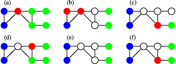
• 62. In what graph among (a) through (f) do the red vertices separate the blue and green vertices?

  

• 63. Let X, Y be binary variables that take zeros and ones and are independent, and let Z be the residue of the sum when divided by two. Show that X, Y are not conditionally independent given Z. Note that the probabilities p and q of $X=1$ and $Y=1$ are not necessarily 0 and 5 and that we do not assume $p=q$.

• 64. For the precision matrix $\Theta =(\theta _{i,j})_{i,j=1,2,3}$, with $\theta _{12}=\theta _{21}=0$, show

  $$\det \Sigma _{\{1,2,3\}}\det \Sigma _{\{3\}}=\det \Sigma _{\{1,3\}}\det \Sigma _{\{2,3\}}\ ,$$

  where by $\Sigma _S$, we mean the submatrix of $\Sigma$ that consists of rows and columns with indices $S\subseteq \{1,2,3\}$.

• 65. Suppose that we express the probability density function of the p Gaussian variables with mean zero and precision matrix $\Theta$ by

  $$f(x)=\sqrt{\frac{\det \Theta }{(2\pi )^{p}}}\exp \left\{ -\frac{1}{2}x^T\Theta x\right\} \quad (x\in {\mathbb R}^p)\ $$

  and let A, B, C be disjoint subsets of $\{1,\ldots ,p\}$. Show that if

  $$\begin{aligned} f_{A\cup C}(x_{A\cup C})f_{B\cup C}(x_{B\cup C})=f_{A\cup B\cup C}(x_{A\cup B\cup C})f_C(x_C) \end{aligned}$$

  (cf. (5.2))

  for arbitrary $x\in {\mathbb R}^p$, then $\theta _{i,j}=0$ with $i\in A,\ j\in B$ and $i\in B,\ j\in A$.

• 66. Suppose that $X\in {\mathbb R}^{N\times p}$ are N samples, each of which has been generated according to the p variable Gaussian distribution $N(0,\Sigma ) \ (\Sigma \in {\mathbb R}^{p\times p})$, and let $S:=\frac{1}{N}X^TX$, $\Theta :=\Sigma ^{-1}$. Show the following statements.

  • (a) Suppose that $\lambda =0$ and $N<p$. Then, no inverse matrix exists for S

    $$\begin{aligned} \Theta ^{-1}-S-\lambda \psi =0 \end{aligned}$$

    (5.30)

    and no maximum likelihood estimate of $\Theta$ exists.

    Hint   The rank of S is at most N, and $S\in {\mathbb R}^{p\times p}$.

  • (b) The trace of $S\Theta$ with $\Theta =(\theta _{s,t})$ can be written as

    $$ \frac{1}{N}\sum _{i=1}^N\left( \sum _{s=1}^p\sum _{t=1}^px_{i,s}\theta _{s,t}x_{i,t}\right) $$

    Hint   If the multiplications AB and BA of matrices A, B are defined, they have an equal trace, and

    $$\mathrm{trace}(S\Theta )=\frac{1}{N}\mathrm{trace}(X^TX\Theta )=\frac{1}{N}\mathrm{trace}(X\Theta X^T)$$

    when $A=X^T$ and $B=X\Theta$.

  • (c) If we express the probability density function of the p Gaussian variables as $f_\Theta (x_{1},\ldots ,x_{p})$, then the log-likelihood $\frac{1}{N}\sum _{i=1}^N\log f_\Theta (x_{i,1},\ldots ,x_{i,p})$ can be written as

    $$\begin{aligned} \frac{1}{2}\{\log \det \Theta -p\log (2\pi )-\mathrm{trace}(S\Theta )\}\ . \end{aligned}$$

    (cf. (5.9))

  • (d) For $\lambda \ge 0$, the maximization of $\displaystyle \frac{1}{N}\sum _{i=1}^N\log f_\Theta (x_i)-\frac{1}{2}\lambda \sum _{s\not =t}|\theta _{s,t}|$ w.r.t. $\Theta$ is that of

    $$\begin{aligned} \log \det \Theta -\mathrm{trace}(S\Theta )-\lambda \sum _{s\not =t}|\theta _{s,t}| \qquad \text{(cf. } \text{(5.10)) }\ . \end{aligned}$$

    (5.31)

• 67. Let $A_{i,j}$ and |B| be the submatrix that excludes the i-th row and j-th column from matrix $A\in {\mathbb R}^{p\times p}$ and the determinant of $B\in {\mathbb R}^{m\times m}$ ($m\le p$), respectively. Then, we have

  $$\begin{aligned} \sum _{j=1}^p (-1)^{k+j}a_{i,j}|A_{k,j}|= \left\{ \begin{array}{ll} |A|,&{}\ i=k\\ 0,&{}\ i\not =k \end{array} \right. \ . \end{aligned}$$

  (cf. (5.11))

  • (a) When $|A|\not =0$, let B be the matrix whose (j, k) element is $b_{j,k}=(-1)^{k+j}|A_{k,j}|/|A|$. Show that AB is the unit matrix. Hereafter, we write this matrix B as $A^{-1}$.

  • (b) Show that if we differentiate |A| by $a_{i,j}$, then it becomes $(-1)^{i+j}|A_{i,j}|$.

  • (c) Show that if we differentiate $\log |A|$ by $a_{i,j}$, then it becomes $(-1)^{i+j}|A_{i,j}|/|A|$, the (j, i)-th element of $A^{-1}$.

  • (d) Show that if we differentiate the trace of $S\Theta$ by the (s, t)-element $\theta _{s,t}$ of $\Theta$, it becomes the (t, s)-th element of S.

    Hint   Differentiate $\mathrm{trace} (S\Theta )=\sum _{i=1}^p\sum _{j=1}^ps_{i,j}\theta _{j,i}$ by $\theta _{s,t}$.

  • (e) Show that the $\Theta$ that maximizes (5.31) is the solution of (5.12), where $\Psi =(\psi _{s,t})$ is $\psi _{s,t}=0$ if $s=t$ and

    $$\displaystyle \psi _{s,t}= \left\{ \begin{array}{ll} 1,&{}\ \theta _{s,t}>0\\ {[-1,1]},&{}\ \theta _{s,t}=0\\ -1,&{}\ \theta _{s,t}<0 \end{array} \right. $$

    otherwise.

    Hint   If we differentiate $\log \det \Theta$ by $\theta _{s,t}$, it becomes the (t, s)-th element of $\Theta ^{-1}$ from (d). However, because $\Theta$ is symmetric, $\Theta ^{-1}$: $\Theta ^T=\Theta \ \Longrightarrow \ (\Theta ^{-1})^T=(\Theta ^{T})^{-1}=\Theta ^{-1}$ is symmetric as well.

• 68. Suppose that we have

  $$\begin{aligned} \Psi =\left[ \begin{array}{c@{\quad }c} \Psi _{1,1}&{}\psi _{1,2}\\ \psi _{2,1}&{}\psi _{2,2} \end{array} \right] \ ,\ S=\left[ \begin{array}{c@{\quad }c} S_{1,1}&{}s_{1,2}\\ s_{2,1}&{}s_{2,2} \end{array} \right] \ ,\ \Theta =\left[ \begin{array}{c@{\quad }c} \Theta _{1,1}&{}\theta _{1,2}\\ \theta _{2,1}&{}\theta _{2,2} \end{array} \right] \nonumber \\ \left[ \begin{array}{c@{\quad }c} W_{1,1}&{}w_{1,2}\\ w_{2,1}&{}w_{2,2} \end{array} \right] \left[ \begin{array}{c@{\quad }c} \Theta _{1,1}&{}\theta _{1,2}\\ \theta _{2,1}&{}\theta _{2,2} \end{array} \right] = \left[ \begin{array}{c@{\quad }c} I_{p-1}&{}0\\ 0&{}1 \end{array} \right] \qquad \text{(cf. } \text{(5.13)) } \end{aligned}$$

  (5.32)

  for $\Psi , \Theta , S\in {\mathbb R}^{p\times p}$ and W such that $W\Theta =I$, where the upper-left part is $(p-1)\times (p-1)$ and we assume that $\theta _{2,2}>0$.

  • (a) Derive

    $$\begin{aligned} w_{1,2}-s_{1,2}-\lambda \psi _{1,2}=0 \qquad \text{(cf. } \text{(5.14)) } \end{aligned}$$

    (5.33)

    and

    $$\begin{aligned} W_{1,1}\theta _{1,2}+w_{1,2}\theta _{2,2}=0 \qquad \text{(cf. } \text{(5.15)) } \end{aligned}$$

    (5.34)

    from the upper-right part of (5.30) and (5.32), respectively.

    Hint   The upper-right part of $\Theta ^{-1}$ is $w_{1,2}$.

  • (b) Let $\displaystyle \beta = \left[ \begin{array}{c} \beta _1\\ \vdots \\ \beta _{p-1} \end{array} \right] :=-\frac{\theta _{1,2}}{\theta _{2,2}}$. Show that from (5.33), (5.34), the two equations are obtained as

    $$\begin{aligned} W_{1,1}\beta -s_{1,2}+\lambda \phi _{1,2}=0 \qquad \text{(cf. } \text{(5.16)) } \end{aligned}$$

    (5.35)
    $$\begin{aligned} w_{1,2}=W_{1,1}\beta \qquad \text{(cf. } \text{(5.17)) } \ , \end{aligned}$$

    (5.36)

    where the j-th element of $\phi _{1,2}\in {\mathbb R}^{p-1}$ is $\displaystyle \left\{ \begin{array}{ll} 1,&{}\ \beta _j>0\\ {[-1,1]},&{}\ \beta _{j}=0\\ -1,&{}\ \beta _{j}<0 \end{array} \right.$.

    Hint   The sign of each element of $\psi _{2,2}\in {\mathbb R}^{p-1}$ is determined by the sign of $\theta _{1,2}$. From $\theta _{2,2}>0$, the signs of $\beta$ and $\theta _{1,2}$ are opposite; thus, $\psi _{1,2}=-\phi _{1,2}$.

• 69. We obtain the solution of (5.30) in the following way: find the solution of (5.35) w.r.t. $\beta$, substitute it into (5.36), and obtain $w_{1,2}$, which is the same as $w_{2,1}$ due to symmetry.

  We repeat the process, changing the positions of $W_{1,1},w_{1,2}$. For $j=1,\ldots ,p$, $W_{1,1}$ is regarded as W except in the j-th row and j-th column, and $w_{1,2}$ is regarded as W in the j-th column except for the j-th element.

  In the last stage, for $j=1,\ldots ,p$, if we take the following one cycle, we obtain the estimate of $\Theta$:

  $$\begin{aligned} \theta _{2,2}&=[w_{2,2}-w_{1,2}\beta ]^{-1} \qquad \text{(cf. } \text{(5.19)) } \end{aligned}$$

  (5.37)
  $$\begin{aligned} \theta _{1,2}&=-\beta \theta _{2,2} \qquad \text{(cf. } \text{(5.20)) } \end{aligned}$$

  (5.38)

  • (a) Let $A:=W_{1,1}\in {\mathbb R}^{(p-1)\times (p-1)}$, $b=s_{1,2}\in {\mathbb R}^{p-1}$, and $c_j:=b_j-\sum _{k\not =j}a_{j,k}\beta _k$. Show that each $\beta _j$ that satisfies (5.35) can be computed via

    $$\begin{aligned} \beta _j= \left\{ \begin{array}{ll} \displaystyle \frac{c_j-\lambda }{a_{j,j}},&{}\ c_j>\lambda \\[1mm] 0,&{}\ -\lambda<c_j<\lambda \\[1mm] \displaystyle \frac{c_j+\lambda }{a_{j,j}},&{}\ c_j<-\lambda \end{array} \right. \qquad \text{(cf. } \text{(5.18)) } \end{aligned}$$

    (5.39)

  • (b) Derive (5.37) from (5.32).

• 70. We construct the graphical Lasso as follows.

  

  Execute each step, and compare the results.

  

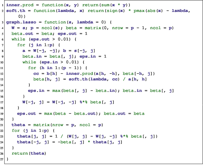
  What rows of the function definition of graph.lasso are the Eqs. (5.36)–(5.39)? Then, we can construct an undirected graph G by connecting each s, t such that $\theta _{s,t}\not =0$ as an edge. Generate the data for $p=5$ and $N=20$ based on a matrix $\Theta =(\theta _{s,t})$ known a priori.

  

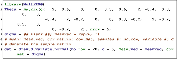
  Moreover, execute the following code, and examine whether the precision matrix $\Theta$ is correctly estimated.

  

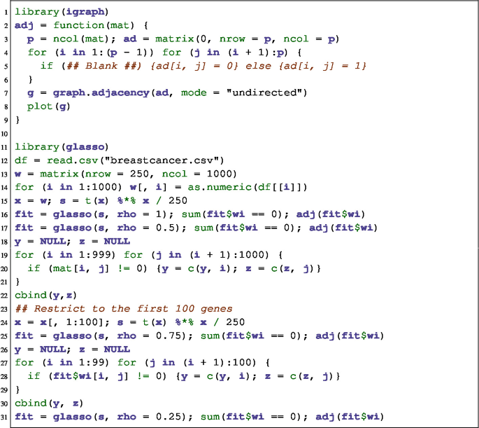
• 71. The function adj defined below connects each (i, j) as an edge if and only if the element is nonzero given a symmetric matrix of size p to construct an undirected graph. Execute it for the breastcancer.csv data.

  

• 72. The following code generates an undirected graph via the quasi-likelihood method and the glmnet package. We examine the difference between using the AND and OR rules, where the original data contains $p=\text{1,000 }$ but the execution is for the first $p=50$ genes to save time. Execute the OR rule case as well as the AND case by modifying the latter.

  

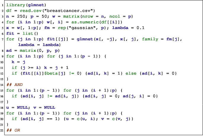
  We execute the quasi-likelihood method for the signs ± of breastcancer.csv.

  

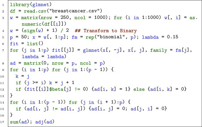
  How can we deal with data that contain both continuous and discrete values?

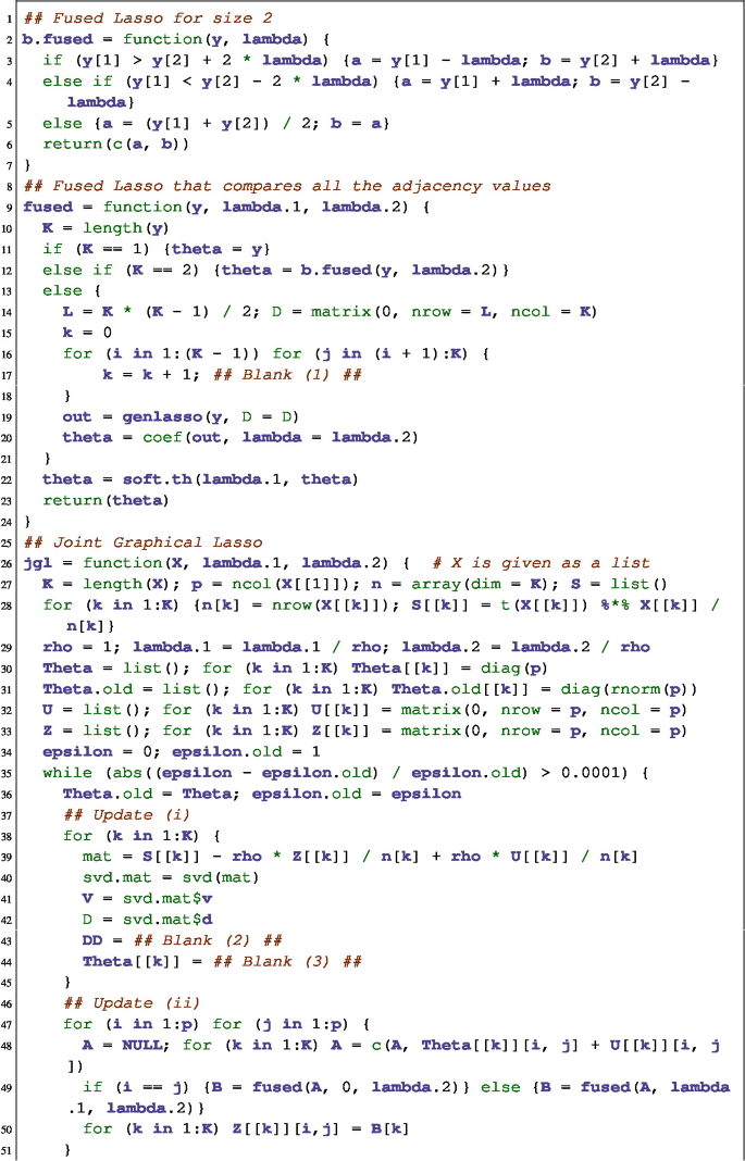
• 73. Joint graphical Lasso (JGL) finds $\Theta _1,\ldots ,\Theta _K$ that maximize

  $$\begin{aligned} \sum _{i=1}^K N_k\{\log \det \Theta _k-\mathrm{trace}(S\Theta _k)\}-P(\Theta _1,\ldots ,\Theta _K) \qquad \text{(cf. } \text{(5.21)) } \end{aligned}$$

  (5.40)

  given $X\in {\mathbb R}^{N\times p}$, $y\in \{1,2,\ldots ,K\}^N \ (K\ge 2$). Suppose that $P(\Theta _1,\ldots ,\Theta _K)$ expresses the fused Lasso penalty

  $$\begin{aligned} P(\Theta _1,\ldots ,\Theta _K):=\lambda _1\sum _{k}\sum _{i\not =j}|\theta _{i,j}^{(k)}|+\lambda _2\sum _{k<k'}\sum _{i,j}|\theta _{i,j}^{(k)}-\theta _{i,j}^{(k')}|\ , \end{aligned}$$

  (cf. (5.22))

  where the indices in $\sum$ range over $k=1,\ldots ,K$, $i,j=1,\ldots ,p$. In JGL, to obtain the solution of (5.40), we apply the ADMM that was introduced in Chap. 4. We define the extended Lagrangian as

  $$\begin{aligned} L_\rho (\Theta ,Z,U):= -\sum _{k=1}^K N_k\{\log \det \Theta _k-\mathrm{trace}(S\Theta _k)\} \end{aligned}$$
  $$\begin{aligned} \qquad \qquad \qquad \,\,+P(Z_1,\ldots ,Z_K)+ \rho \sum _{k=1}^K<U_k,\Theta _k-Z_k>+\frac{\rho }{2}\sum _{k=1}^K \Vert \Theta _k-Z_k\Vert _F^2\ \end{aligned}$$

  (cf. (5.23))

  and repeat the following steps:

  • i. $\Theta ^{(t)}\leftarrow \mathrm{argmin}_\Theta L_\rho (\Theta ,Z^{(t-1)},U^{(t-1)})$

  • ii. $Z^{(t)}\leftarrow \mathrm{argmin}_Z L_\rho (\Theta ^{(t)},Z,U^{(t-1)})$

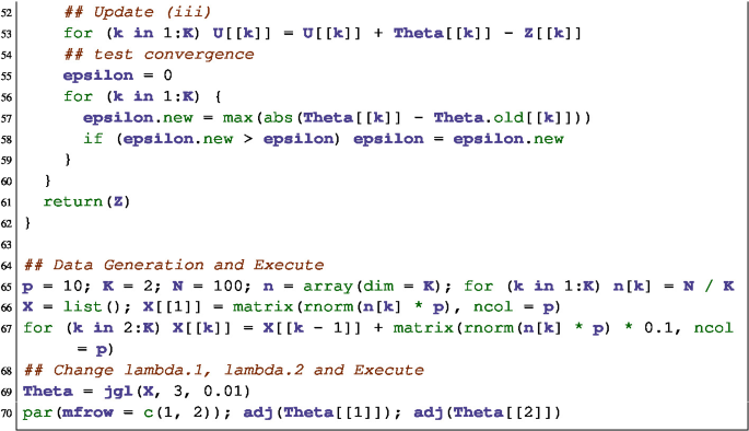
  • iii. $U^{(t)}\leftarrow U^{(t-1)}+\rho (\Theta ^{(t)}-Z^{(t)})$

  More precisely, setting $\rho >0$ and letting $\Theta _k$ and $Z_k,U_k$ be the unit and zero matrices $k=1,\ldots ,K$, respectively, repeat the above three steps.

  • (a) Show that if we differentiate (5.40) by $\Theta _k$ in the first step, then we have

    $$-N_k(\Theta _k^{-1}-S_k)+\rho (\Theta _k-Z_k+U_k)=0\ .$$

  • (b) We wish to obtain the optimum $\Theta _k$ in the first step. To this end, we decompose both sides of the symmetric matrix

    $$\Theta _k^{-1}-\frac{\rho }{N_k}\Theta _k=S_k-\rho \frac{Z_k}{N_k}+\rho \frac{U_k}{N_k}$$

    as $VDV^T$ and obtain $\tilde{D}$ such that

    $$\tilde{D}_{j,j}=\frac{N_k}{2\rho }(-D_{j,j}+\sqrt{D_{j,j}^2+4\rho /N_k})$$

    from the diagonal matrix D. Show that $V\tilde{D}V^T$ is the optimum $\Theta$.

  • (c) In the second step, for $K=2$, we require a fused Lasso procedure for two values. Let $y_1,y_2$ be the two sets of data. Derive $\theta _1,\theta _2$ that minimize

    $$\frac{1}{2}(y_1-\theta _1)^2+\frac{1}{2}(y_2-\theta _2)^2+|\theta _1-\theta _2|\ .$$

• 74. We construct the fused Lasso JGL. Fill in the blanks, and execute the procedure.

  

  

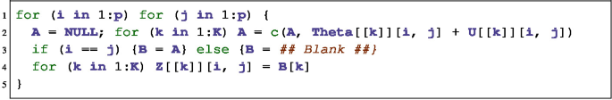
• 75. For the group Lasso, only the second step should be replaced. Let $A_k[i,j]=\Theta _k[i,j]+U_k[i,j]$. Then, no update is required for $i=j$, and

  $$Z_k[i,j]=\mathcal{S}_{\lambda _1/\rho }(A_k[i,j])\left( 1-\frac{\lambda _2}{\rho \sqrt{\sum _{k=1}^K \mathcal{S}_{\lambda _1/\rho }(A_k[i,j])^2}}\right) _+$$

  for $i\not =j$. We construct the code. Fill in the blank, and execute the procedure as in the previous exercise.