Support Vector Machine

Abstract

Support vector machine is a method for classification and regression that draws an optimal boundary in the space of covariates (p dimension) when the samples (x ₁, y ₁), …, (x _N, y _N) are given. This is a method to maximize the minimum value over i = 1, …, N of the distance between x _i and the boundary. This notion is generalized even if the samples are not separated by a surface by softening the notion of a margin. Additionally, by using a general kernel that is not the inner product, even if the boundary is not a surface, we can mathematically formulate the problem and obtain the optimum solution. In this chapter, we consider only the two-class case and focus on the core part. Although omitted here, the theory of support vector machines also applies to regression and classification with more than two classes.

Appendices

Appendix: Proofs of Propositions

Proposition 23

The distance between a point $(x,y)\in {\mathbb R}^2$ and a line l : aX + bY + c = 0, $a,b\in {\mathbb R}$ is given by

$$\displaystyle \begin{aligned}\displaystyle \frac{|ax+by+c|}{\sqrt{a^2+b^2}}\ .\end{aligned}$$

Proof

Let (x ₀, y ₀) be the perpendicular foot of l from (x, y). l′ is a normal of l and can be written by

$$\displaystyle \begin{aligned}l': \frac{X-x_0}{a}=\frac{Y-y_0}{b}=t\end{aligned}$$

for some t (Fig. 9.6). Since (x ₀, y ₀) and (x, y) are on l and l′, respectively, we have

$$\displaystyle \begin{aligned}\left\{ \begin{array}{l} \displaystyle ax_0+by_0+c=0\\ {} \displaystyle \frac{x-x_0}{a}=\frac{y-y_0}{b}=t \ . \end{array} \right. \end{aligned}$$

Fig. 9.6

The distance between a point and a line $\sqrt {(x-x_0)^2+(y-y_0)^2}$, where l′ is the normal of l that goes through (x ₀, y ₀)

If we erase (x ₀, y ₀), from x ₀ = x − at, y ₀ = y − bt, a(x − at) + b(y − bt) + c = 0, we have t = (ax + by + c)∕(a ² + b ²). Thus, the distance is

$$\displaystyle \begin{aligned}\sqrt{(x-x_0)^2+(y-y_0)^2}=\sqrt{(a^2+b^2)t^2}=\frac{|ax+by+c|}{\sqrt{a^2+b^2}}\ .\end{aligned}$$

□

Proposition 25

$$\displaystyle \begin{aligned}\left\{ \begin{array}{lll} \alpha_i=0&\Longleftarrow &y_i(\beta_0+x_i\beta)> 1\\ 0<\alpha_i<C&\Longrightarrow &y_i(\beta_0+x_i\beta)=1\\ \alpha_i=C&\Longleftarrow &y_i(\beta_0+x_i\beta)< 1. \end{array} \right. \end{aligned}$$

Proof

When α _i = 0, applying (9.20), (9.17), and (9.14) in this order, we have

$$\displaystyle \begin{aligned}\alpha_i=0 \Longrightarrow \mu_i=C>0 \Longrightarrow \epsilon_i=0 \Longrightarrow y_i(\beta_0+x_i\beta)\geq 1\ .\end{aligned}$$

When 0 < α _i < C, from (9.17) and (9.20), we have 𝜖 _i = 0. Moreover, applying (9.16), we have

$$\displaystyle \begin{aligned}0<\alpha_i<C \Longrightarrow y_i(\beta_0+x_i\beta)-(1-\epsilon_i)=0 \Longrightarrow y_i(\beta_0+x_i\beta)=1\ .\end{aligned}$$

When α _i = C, from (9.15), we have 𝜖 _i ≥ 0. Moreover, applying (9.16), we have

$$\displaystyle \begin{aligned}\alpha_i=C \Longrightarrow y_i(\beta_0+x_i\beta)-(1-\epsilon_i)=0 \Longrightarrow y_i(\beta_0+x_i\beta)\leq 1\ .\end{aligned}$$

Furthermore, from (9.16), we have y _i(β ₀ + x _i β) > 1⇒α _i = 0. On the other hand, applying (9.14), (9.17), and (9.20) in this order, we have

$$\displaystyle \begin{aligned}y_i(\beta_0+x_i\beta)< 1 \Longrightarrow \epsilon_i>0 \Longrightarrow \mu_i=0 \Longrightarrow \alpha_i=C\ .\end{aligned}$$

□

Exercises 75–87

We define the distance between a point $(u,v)\in {\mathbb R}^2$ and a line $aU+bV+c=0,\ a,b\in {\mathbb R}$ by

$$\displaystyle \begin{aligned}\displaystyle \frac{|au+bv+c|}{\sqrt{a^2+b^2}}\ .\end{aligned}$$

For $\beta \in {\mathbb R}^p$ such that $\beta _0\in {\mathbb R}$ and ∥β∥₂ = 1, when samples $(x_1,y_1),\ldots ,(x_N,y_N)\in {\mathbb R}^p\times \{-1,1\}$ satisfy the separability y ₁(β ₀ + x ₁ β), …, y _N(β ₀ + x _N β) ≥ 0, the support vector machine is formulated as the problem of finding (β ₀, β) that maximize the minimum value M :=min_i y _i(β ₀ + x _i β) over the distances between x _i (row vector) and the surface β ₀ + Xβ = 0.

• 75. We extend the support vector machine problem to finding $(\beta _0,\beta )\in {\mathbb R}\times {\mathbb R}^p$ and 𝜖 _i ≥ 0, i = 1, …, N, that maximize M under the constraints γ ≥ 0, M ≥ 0, $\displaystyle \sum _{i=1}^N\epsilon _i\leq \gamma$, and

  $$\displaystyle \begin{aligned}y_i(\beta_0+x_i\beta)\geq M(1-\epsilon_i) ,\ i=1,\ldots,N\ .\end{aligned} $$

  • (a) What can we say about the locations of samples (x _i, y _i) when 𝜖 _i = 0, 0 < 𝜖 _i < 1, 𝜖 _i = 1, 1 < 𝜖 _i.

  • (b) Suppose that y _i(β ₀ + x _i β) < 0 for at least r samples and for any β ₀ and β. Show that if γ ≤ r, then no solution exists. Hint: 𝜖 _i > 1 for such an i.

  • (c) The larger the γ is, the smaller the M. Why?

• 76. We wish to obtain $\beta \in {\mathbb R}^p$ that minimizes f ₀(β) under f _j(β) ≤ 0, j = 1, …, m. If such a solution exists, we denote the minimum value by f ^∗. Consider the following two equations

  $$\displaystyle \begin{aligned} \begin{array}{rcl} \sup_{\alpha\geq 0}L(\alpha,\beta)&=& \left\{ \begin{array}{l@{\quad }l} f_0(\beta),&f_j(\beta)\leq 0\ ,\ j=1,\ldots,m\\ +\infty&\text{Otherwise} \end{array} \right. \end{array} \end{aligned} $$

  (9.25)
  $$\displaystyle \begin{aligned} \begin{array}{rcl} f^*&:=&\inf_\beta\sup_{\alpha\geq 0}L(\alpha,\beta)\geq\sup_{\alpha\geq 0}\inf_\beta L(\alpha,\beta) {} \end{array} \end{aligned} $$

  (9.26)

  under

  $$\displaystyle \begin{aligned}L(\alpha,\beta):=f_0(\beta)+\sum_{j=1}^m \alpha_jf_j(\beta)\end{aligned}$$

  for $\alpha =(\alpha _1,\ldots ,\alpha _m)\in {\mathbb R}^m$. Moreover, suppose p = 2 and m = 1. For

  $$\displaystyle \begin{aligned} L(\alpha,\beta):=\beta_1+\beta_2+\alpha(\beta_1^2+\beta_2^2-1)\ , \end{aligned} $$

  (9.27)

  such that the equality holds in the inequality (9.26).

• 77. Suppose that $f_0,f_1,\ldots ,f_m: {\mathbb R}^p\rightarrow {\mathbb R}$ are convex and differentiable at β = β ^∗. It is known that $\beta ^*\in {\mathbb R}^p$ is the optimum value of $\displaystyle \min \{f_0(\beta )\mid f_i(\beta )\leq 0,\ i=1,\ldots ,m\}$ if and only if there exist α _i ≥ 0, i = 1, …, m, such that

  $$\displaystyle \begin{aligned} f_i(\beta^*)\leq 0 ,\ i=1,\ldots,m, \end{aligned} $$

  (9.28)

  and the two conditions are met (KKT conditions)

  $$\displaystyle \begin{aligned} \begin{array}{rcl} & \alpha_if_i(\beta^*)=0 ,\ i=1,\ldots,m, {} \end{array} \end{aligned} $$

  (9.29)
  $$\displaystyle \begin{aligned} \begin{array}{rcl} & \displaystyle \nabla f_0(\beta^*)+\sum_{i=1}^m \alpha_i\nabla f_i(\beta^*)=0. {} \end{array} \end{aligned} $$

  (9.30)

  In this problem, we consider the sufficiency.

  • (a) If $f: {\mathbb R}^p\rightarrow {\mathbb R}$ is convex and differentiable at $x=x_0\in {\mathbb R}$, then

    $$\displaystyle \begin{aligned} f(x)\geq f(x_0)+\nabla f(x_0)^T(x-x_0) \end{aligned} $$

    (9.31)

    for each $x\in {\mathbb R}^p$. From this fact, show that f ₀(β ^∗) ≤ f ₀(β) for arbitrary $\beta \in {\mathbb R}^p$ that satisfies (9.28). Hint: Use (9.29) and (9.30) once, (9.31) twice, and f ₁(β) ≤ 0, …, f _m(β) ≤ 0 once.

  • (b) For (9.27), find the conditions that correspond to (9.28)–(9.30).

• 78. If we remove the condition ∥β∥₂ = 1 in Problem 75 and regard β ₀∕M, β∕M as β ₀ and β, then the problem reduces to finding β ₀, β, 𝜖 _i, i = 1, …, N, that minimize

  $$\displaystyle \begin{aligned} L_P:=\frac{1}{2}\|\beta\|{}^2_2+C\sum_{i=1}^N\epsilon_i-\sum_{i=1}^N\alpha_i\{ y_i(\beta_0+x_i\beta)-(1-\epsilon_i)\}-\sum_{i=1}^N\mu_i\epsilon_i\ , \end{aligned} $$

  (9.32)

  where C > 0 (cost), the last two terms are constraints, and α _i, μ _i ≥ 0, i = 1, …, N, are the Lagrange coefficients. Show that the KKT conditions (9.28)–(9.30) are the following:

  $$\displaystyle \begin{aligned} \begin{array}{rcl} & \displaystyle \sum_{i=1}^N\alpha_iy_i=0 {} \end{array} \end{aligned} $$

  (9.33)
  $$\displaystyle \begin{aligned} \begin{array}{rcl} & \displaystyle \beta=\sum_{i=1}^N\alpha_iy_ix_i\in {\mathbb R}^p {} \end{array} \end{aligned} $$

  (9.34)
  $$\displaystyle \begin{aligned} \begin{array}{rcl} & C-\alpha_i-\mu_i=0 {} \end{array} \end{aligned} $$

  (9.35)
  $$\displaystyle \begin{aligned} \begin{array}{rcl} & \alpha_i[y_i(\beta_0+x_i\beta)-(1-\epsilon_i)]=0 {} \end{array} \end{aligned} $$

  (9.36)
  $$\displaystyle \begin{aligned} \begin{array}{rcl} & \mu_i\epsilon_i=0 {} \end{array} \end{aligned} $$

  (9.37)
  $$\displaystyle \begin{aligned} \begin{array}{rcl} & y_i(\beta_0+x_i\beta)-(1-\epsilon_i)\geq 0 {} \end{array} \end{aligned} $$

  (9.38)
  $$\displaystyle \begin{aligned} \begin{array}{rcl} & \epsilon_i\geq 0. {} \end{array} \end{aligned} $$

  (9.39)

• 79. Show that the dual problem (9.32) of L _P is given by

  $$\displaystyle \begin{aligned} L_D:=\sum_{i=1}^N\alpha_i-\frac{1}{2}\sum_{i=1}^N\sum_{j=1}^N\alpha_i\alpha_jy_iy_jx_i^Tx_j\ , \end{aligned} $$

  (9.40)

  where α ranges over (9.33) and

  $$\displaystyle \begin{aligned} 0\leq \alpha_i\leq C\ . \end{aligned} $$

  (9.41)

  Moreover, how is β obtained from such an α?

• 80. Show the following:

  $$\displaystyle \begin{aligned}\left\{ \begin{array}{lll} \alpha_i=0&\Longleftarrow &y_i(\beta_0+x_i\beta)> 1\\ 0<\alpha_i<C&\Longrightarrow &y_i(\beta_0+x_i\beta)=1\\ \alpha_i=C&\Longleftarrow &y_i(\beta_0+x_i\beta)< 1. \end{array} \right. \end{aligned}$$

• 81. We wish to obtain the value of β ₀ by y _i(β ₀ + x _i β) = 1 for at least one i.

  • (a) Show that α ₁ = ⋯ = α _N = 0 and y _i(β ₀ + x _i β) = 1 imply β ₀ = y _i, i = 1, …, N.

  • (b) Suppose that (α = 0 or α = C) and y _i(β ₀ + x _i β) ≠ 1 for each i, and let 𝜖 _∗ :=min_i 𝜖 _i. Show that L _p decreases when replacing 𝜖 _i and β by 𝜖 _i − 𝜖 _∗ and β ₀ + y _i 𝜖 _∗, respectively, for each i, which means that no optimum solution can be obtained under the assumption. Hint: $y_i=\pm 1\Longleftrightarrow y_i^2=1$.

  • (c) Show that y _i(β ₀ + x _i β) = 1 for at least one i.

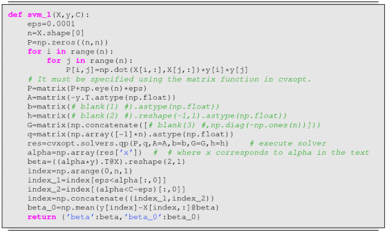
• 82. In order to input the dual problem (9.40), (9.33), and (9.41) into a quadratic programming solver, we specify $D_{\mathit {mat}}\in {\mathbb R}^{N\times N}$, $A_{\mathit {mat}}\in {\mathbb R}^{m\times N}$, $d_{\mathit {vec}}\in {\mathbb R}^N$, and $b_{\mathit { vec}}\in {\mathbb R}^m$ (m ≥ 1) such that

  $$\displaystyle \begin{aligned}L_D=-\frac{1}{2}\alpha^TD_{\mathit{mat}}\alpha+d_{\mathit{vec}}^T\alpha\end{aligned}$$
  $$\displaystyle \begin{aligned}A_{\mathit{mat}}\alpha\geq b_{\mathit{vec}}\ ,\end{aligned}$$

  where the first meq and the last m − meq are equalities and inequalities, respectively, in the m constraints A _mat α ≥ b _vec, $\alpha \in {\mathbb R}^N$. If we define

  $$\displaystyle \begin{aligned}b_{\mathit{vec}}:=[0,-C,\ldots,-C,0,\ldots,0]^T,\end{aligned}$$

  what are D _mat, A _mat, d _vec, and meq? Moreover, fill in the blanks below and execute the result.

  

• 83. Let V  be a vector space. We define a kernel K(x, y) w.r.t. $\phi : {\mathbb R}^p\rightarrow V$ as the inner product of ϕ(x) and ϕ(y) given $(x,y)\in {\mathbb R}^p\times {\mathbb R}^p$. For example, for the d-dimensional polynomial kernel K(x, y) = (1 + x ^T y)^d, if d = 1 and p = 2, then the mapping is

  $$\displaystyle \begin{aligned}((x_1,x_2), (y_1,y_2))\mapsto 1\cdot 1+x_1y_1+x_2y_2=(1,x_1,x_2)^T(1,y_1,y _2)\ .\end{aligned}$$

  In this case, we regard the map ϕ as (x ₁, x ₂)↦(1, x ₁, x ₂). What is ϕ for p = 2 and d = 2? Write a Python function K_poly(x,y) that realizes the d = 2-dimensional polynomial kernel.

• 84. Let V  be a vector space over $\mathbb R$.

  • (a) Suppose that V  is the set of continuous functions in [0, 1]. Show that $\displaystyle \int _0^1 f(x)g(x)dx$, f, g ∈ V , is an inner product of V .

  • (b) For vector space $V:={\mathbb R}^p$, show that (1 + x ^T y)², $x,y \in {\mathbb R}^p$, is not an inner product of V .

  • (c) Write a Python function K_linear(x,y) for the standard inner product.

  Hint: Check the definition of an inner product, for a, b, c ∈ V , $\alpha \in {\mathbb R}$, 〈a + b, c〉 = 〈a, c〉 + 〈b, c〉; 〈a, b〉 = 〈b, a〉; 〈αa, b〉 = α〈a, b〉; 〈a, a〉 = ∥a∥² ≥ 0.

• 85. In the following, using $\phi : {\mathbb R}^p\rightarrow V$, we replace $x_i\in {\mathbb R}^p$, i = 1, …, N, with ϕ(x _i) ∈ V . Thus, $\beta \in {\mathbb R}^p$ is expressed as $\beta =\sum _{i=1}^N\alpha _iy_i\phi (x_i)\in V$, and the inner product 〈x _i, x _j〉 in L _D is replaced by the inner product of ϕ(x _i) and ϕ(x _j), i.e., K(x _i, x _j). If we extend the vector space, the border ϕ(X)β + β ₀ = 0, i.e., $\sum _{i=1}^N\alpha _iy_iK(X,x_i)+\beta _0=0,$ is not necessarily a surface. Modify the svm_1 in Problem 82 as follows:

  • (a) add argument K to the definition,

  • (b) replace np.dot(X[,i]∗X[,j]) with K(X[i,],X[j,]), and

  • (c) replace beta in return by alpha.

  Then, execute the function svm_2 by filling in the blanks.

  

       pcost       dcost       gap    pres   dres  0: -7.5078e+01 -6.3699e+02  4e+03  4e+00  3e-14  1: -4.5382e+01 -4.5584e+02  9e+02  6e-01  2e-14  2: -2.6761e+01 -1.7891e+02  2e+02  1e-01  1e-14  3: -2.0491e+01 -4.9270e+01  4e+01  2e-02  1e-14  4: -2.4760e+01 -3.3429e+01  1e+01  5e-03  5e-15  5: -2.6284e+01 -2.9464e+01  4e+00  1e-03  3e-15  6: -2.7150e+01 -2.7851e+01  7e-01  4e-05  4e-15  7: -2.7434e+01 -2.7483e+01  5e-02  2e-06  5e-15  8: -2.7456e+01 -2.7457e+01  5e-04  2e-08  5e-15  9: -2.7457e+01 -2.7457e+01  5e-06  2e-10  6e-15 Optimal solution found.      pcost       dcost       gap    pres   dres  0: -9.3004e+01 -6.3759e+02  4e+03  4e+00  4e-15  1: -5.7904e+01 -4.6085e+02  8e+02  5e-01  4e-15  2: -3.9388e+01 -1.5480e+02  1e+02  6e-02  1e-14  3: -4.5745e+01 -6.8758e+01  3e+01  9e-03  3e-15  4: -5.0815e+01 -6.0482e+01  1e+01  3e-03  2e-15  5: -5.2883e+01 -5.7262e+01  5e+00  1e-03  2e-15  6: -5.3646e+01 -5.6045e+01  3e+00  6e-04  2e-15  7: -5.4217e+01 -5.5140e+01  1e+00  2e-04  2e-15  8: -5.4531e+01 -5.4723e+01  2e-01  1e-05  2e-15  9: -5.4617e+01 -5.4622e+01  6e-03  3e-07  3e-15 10: -5.4619e+01 -5.4619e+01  6e-05  3e-09  3e-15 11: -5.4619e+01 -5.4619e+01  6e-07  3e-11  2e-15 Optimal solution found.

   

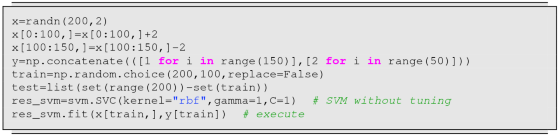
  • (a) Execute the support vector machine with γ = 1 and C = 100.

    

  • (b) Use the GridSearchCV cosmmand to find the optimal C and γ over C = 0.1, 1, 10, 100, 1000 and γ = 0.5, 1, 2, 3, 4 via cross-validation.

    

    GridSearchCV(cv=10, error_score='raise-deprecating',              estimator=SVC(C=1.0, cache_size=200, class_weight=None, coef0=0.0,                            decision_function_shape='ovr', degree=3,                            gamma='auto_deprecated', kernel='rbf', max_iter=-1,                            probability=False, random_state=None, shrinking=True,                            tol=0.001, verbose=False),              iid='warn', n_jobs=None,              param_grid={'C': [0.1, 1, 10, 100, 1000],                          'gamma': [0.5, 1, 2, 3, 4]},              pre_dispatch='2∗n_jobs', refit=True, return_train_score=False,              scoring=None, verbose=0)

• 86. A support vector machine works even when more than two classes exist. In fact, the function svm in the sklearn packages runs even if we give no information about the number of classes. Fill in the blanks and execute it.

  

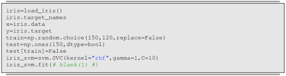
  SVC(C=10, cache_size=200, class_weight=None, coef0=0.0,     decision_function_shape='ovr', degree=3, gamma=1, kernel='rbf', max_iter=-1,     probability=False, random_state=None, shrinking=True, tol=0.001,     verbose=False)

  

  array([[ 9.,  0.,  0.],        [ 0., 10.,  0.],        [ 0.,  3.,  8.]])