Nonlinear Regression

Abstract

For regression, until now we have focused on only linear regression, but in this chapter, we will consider the nonlinear case where the relationship between the covariates and response is not linear. In the case of linear regression in Chap. 2, if there are p variables, we calculate p + 1 coefficients of the basis that consists of p + 1 functions 1, x ₁, ⋯ , x _p. This chapter addresses regression when the basis is general. For example, if the response is expressed as a polynomial of the covariate x, the basis consists of 1, x, ⋯ , x ^p. We also consider spline regression and find a basis. In that case, the coefficients can be found in the same manner as for linear regression. Moreover, we consider local regression for which the response cannot be expressed by a finite number of basis functions. Finally, we consider a unified framework (generalized additive model) and backfitting.

Appendix: Proofs of Propositions

Proposition 20

The function f(x) has K cubic polynomials h ₁(x) = 1, h ₂(x) = x, h _j+2(x) = d _j(x) − d _K−1(x), j = 1, …, K − 2, as a basis, and if we define

$$\displaystyle \begin{aligned}\gamma_1:=\beta_1,\ \gamma_2:=\beta_2,\ \gamma_3:=(\alpha_K-\alpha_1)\beta_3,\ \ldots,\ \gamma_K:=(\alpha_K-\alpha_{K-2})\beta_K\end{aligned}$$

for each β ₁, …, β _K , we can express f as $\displaystyle f(x)=\sum _{j=1}^K\gamma _j h_j(x)$ , where we have

$$\displaystyle \begin{aligned}d_j(x)=\frac{(x-\alpha_j)^3_+-(x-\alpha_K)_+^3}{\alpha_K-\alpha_j} ,\ j=1,\ldots,K-1\ .\end{aligned}$$

Proof

First, the condition (7.3) $\displaystyle \beta _{K+1}=-\sum _{j=3}^K\frac {\alpha _K-\alpha _{j-2}}{\alpha _K-\alpha _{K-1}}\beta _j$ can be expressed as

$$\displaystyle \begin{aligned} \gamma_{K+1}=-\sum_{j=3}^K\gamma_j \end{aligned} $$

(7.9)

with γ _K+1 := (α _K − α _K−1)β _K+1. □

In the following, we show that γ ₁, …, γ _K are coefficients when the basis consists of h ₁(x) = 1, h ₂(x) = x, h _j+2(x) = d _j(x) − d _K−1(x), j = 1, …, K − 2, where

$$\displaystyle \begin{aligned}d_j(x)=\frac{(x-\alpha_j)^3_+-(x-\alpha_K)_+^3}{\alpha_K-\alpha_j} ,\ j=1,\ldots,K-1\end{aligned}$$

for each case of x ≤ α _K and α _K ≤ x.

In fact, for x ≤ α _K, using (7.9), we obtain

$$\displaystyle \begin{aligned} \begin{array}{rcl} \sum_{j=3}^{K+1}\gamma_j\frac{(x-\alpha_{j-2})_+^3}{\alpha_K-\alpha_{j-2}}& =&\displaystyle \sum_{j=3}^{K}\gamma_j\frac{(x-\alpha_{j-2})_+^3}{\alpha_K-\alpha_{j-2}} -\sum_{j=3}^{K}\gamma_j\frac{(x-\alpha_{K-1})_+^3}{\alpha_K-\alpha_{K-1}}\\ & =&\displaystyle \sum_{j=3}^{K}\gamma_j\left\{\frac{(x-\alpha_{j-2})_+^3}{\alpha_K-\alpha_{j-2}} -\frac{(x-\alpha_{K-1})_+^3}{\alpha_K-\alpha_{K-1}}\right\}\\ & =&\displaystyle \sum_{j=3}^K \gamma_j\{d_{j-2}(x)-d_{K-1}(x)\}\ , \end{array} \end{aligned} $$

which means

$$\displaystyle \begin{aligned} \begin{array}{rcl} f(x)& =&\displaystyle \beta_1+\beta_2x+\sum_{j=3}^{K+1}\beta_j(x-\alpha_{j-2})_+^3\\ & =&\displaystyle \gamma_1+\gamma_2x+\sum_{j=3}^{K+1}\gamma_j\frac{(x-\alpha_{j-2})_+^3}{\alpha_K-\alpha_{j-2}}\\ & =&\displaystyle \gamma_1+\gamma_2x+\sum_{j=3}^{K}\gamma_j(d_{j-2}(x)-d_{K-1}(x))=\sum_{j=1}^K\gamma_j h_j(x)\ . \end{array} \end{aligned} $$

For x ≥ α _K, according to the definition, and j = 1, …, K − 2, we have

$$\displaystyle \begin{aligned} \begin{array}{rcl} h_{j+2}(x)& =&\displaystyle \frac{(x-\alpha_j)^3-(x-\alpha_K)^3}{\alpha_K-\alpha_j} - \frac{(x-\alpha_{K-1})^3-(x-\alpha_K)^3}{\alpha_K-\alpha_{K-1}}\\ & =&\displaystyle (x-\alpha_j)^2+(x-\alpha_K)^2+(x-\alpha_j)(x-\alpha_K)-(x-\alpha_K)^2\\ & &\displaystyle -(x-\alpha_{K-1})^2-(x-\alpha_{K-1})(x-\alpha_K)\\ & =&\displaystyle (\alpha_{K-1}-\alpha_j)(2x-\alpha_j-\alpha_{K-1})+(x-\alpha_K)(\alpha_{K-1}-\alpha_j)\qquad \end{array} \end{aligned} $$

(7.10)

$$\displaystyle \begin{aligned} \begin{array}{rcl} & =&\displaystyle (\alpha_{K-1}-\alpha_j)(3x-\alpha_j-\alpha_{K-1}-\alpha_K){}\ , \end{array} \end{aligned} $$

(7.11)

where the second to last equality is obtained by factorization between the first and fourth terms and between the third and sixth terms. Therefore, if we substitute x = α _K into $f(x)=\sum _{j=1}^K\gamma _jh_j(x)$ and $f'(x)=\sum _{j=1}^K\gamma _jh_j^{\prime }(x)$, we obtain

$$\displaystyle \begin{aligned} f(\alpha_K)=\gamma_1+\gamma_2\alpha_K+\sum_{j=3}^K\gamma_j(\alpha_{K-1}-\alpha_{j-2})(2\alpha_K-\alpha_{j-2}-\alpha_{K-1}) \end{aligned} $$

(7.12)

and

$$\displaystyle \begin{aligned} f'(\alpha_K)=\gamma_2+3\sum_{j=3}^K\gamma_j(\alpha_{K-1}-\alpha_{j-2}). \end{aligned} $$

(7.13)

Thus, for x ≥ α _K, we have shown that $f(x)=\sum _{j=1}^K\gamma _jh_j(x)$ is such a line. On the other hand, using the function $\displaystyle f(x)=\gamma _1+\gamma _2x+\sum _{j=1}^{K+1}\gamma _j\frac {(x-\alpha _{j-2})_+^3}{\alpha _K-\alpha _{j-2}}$ for x ≤ α _K, to compute the value and its derivative at x = α _K, from (7.9), we obtain

$$\displaystyle \begin{aligned} \begin{array}{rcl} f(\alpha_K)& =&\displaystyle \gamma_1+\gamma_2\alpha_K+\sum_{j=3}^{K+1}\gamma_j\frac{(\alpha_K-\alpha_{j-2})^3}{\alpha_K-\alpha_{j-2}} =\gamma_1+\gamma_2\alpha_K+\sum_{j=3}^{K+1}\gamma_j(\alpha_K-\alpha_{j-2})^2\qquad \\ \end{array} \end{aligned} $$

(7.14)

$$\displaystyle \begin{aligned} \begin{array}{rcl} & =&\displaystyle \gamma_1+\gamma_2\alpha_K+\sum_{j=3}^{K}\gamma_j(\alpha_K-\alpha_{j-2})^2-\sum_{j=3}^{K}\gamma_j(\alpha_K-\alpha_{K-1})^2 \\ & =&\displaystyle \gamma_1+\gamma_2\alpha_K+\sum_{j=3}^{K}\gamma_j(\alpha_{K-1}-\alpha_{j-2})(2\alpha_K-\alpha_{j-2}-\alpha_{K-1}){} \end{array} \end{aligned} $$

(7.15)

and

$$\displaystyle \begin{aligned} \begin{array}{rcl} f'(\alpha_K)& =&\displaystyle \gamma_2+3\sum_{j=3}^{K+1}\gamma_j\frac{(\alpha_K-\alpha_{j-2})^2}{\alpha_K-\alpha_{j-2}}= \gamma_2+3\sum_{j=3}^{K+1}\gamma_j(\alpha_K-\alpha_{j-2}){}\qquad \qquad \\ & =&\displaystyle \gamma_2+3\sum_{j=3}^K\gamma_j(\alpha_K-\alpha_{j-2})-3\sum_{j=3}^K\gamma_j(\alpha_K-\alpha_{K-1}) \\ & =&\displaystyle \gamma_2+3\sum_{j=3}^K\gamma_j(\alpha_{K-1}-\alpha_{j-2}). \end{array} \end{aligned} $$

(7.16)

Since not only (7.12) and (7.15) but also (7.13) and (7.16) coincide, the proposition holds even for x ≥ α _K.

Proposition 21 (Green and Silverman, 1994)

The natural spline f with knots x ₁, …, x _N minimizes L(f).

Proof

Let f(x) be an arbitrary function that minimizes (7.5), g(x) be the natural spline with knots x ₁, …, x _N, and r(x) := f(x) − g(x). Since the dimension of g(x) is N, we can determine the coefficients γ ₁, …, γ _N of the basis functions h ₁(x), …, h _N(x) in $g(x)=\sum _{i=1}^N\gamma _ih_i(x)$ such that

$$\displaystyle \begin{aligned}g(x_1)=f(x_1),\ldots, g(x_N)=f(x_N).\end{aligned}$$

In fact, we can solve the following linear equation:

$$\displaystyle \begin{aligned} \begin{array}{rcl} \left[ \begin{array}{c@{\quad }c@{\quad }c} h_1(x_1)& \cdots&\displaystyle h_N(x_1)\\ \vdots& \ddots&\displaystyle \vdots\\ h_1(x_N)& \cdots&\displaystyle h_N(x_N)\\ \end{array} \right] \left[ \begin{array}{c} \gamma_1\\ \vdots\\ \gamma_N\\ \end{array} \right] = \left[ \begin{array}{c} f(x_1)\\ \vdots\\ f(x_N)\\ \end{array} \right]\ . \end{array} \end{aligned} $$

Then, note that we have r(x ₁) = ⋯ = r _N(x _N) = 0 and that g(x) is a line and a cubic polynomial for x ≤ x ₁, x _N ≤ x and inside these values, respectively, which means that g ^′′′(x) is a constant γ _i for each interval [x _i, x _i+1], specifically, g ^′′(x ₁) = g ^′′(x _N) = 0. Thus, we have

$$\displaystyle \begin{aligned}\int_{x_1}^{x_N} g^{\prime\prime}(x)r^{\prime\prime}(x)dx=[g^{\prime\prime}(x)r'(x)]_{x_1}^{x_N}-\int_{x_1}^{x_N} g^{\prime\prime\prime}(x)r'(x)dx=-\sum_{i=1}^{N-1} \gamma_i[r(x)]_{x_{i}}^{x_{i+1}}=0\ . \end{aligned}$$

Hence, we have

$$\displaystyle \begin{aligned} \begin{array}{rcl} \int_{-\infty}^{\infty}\{f^{\prime\prime}(x)\}^2dx& \geq&\displaystyle \int_{x_1}^{x_N} \{g^{\prime\prime}(x)+r^{\prime\prime}(x)\}^2dx\\ & \geq&\displaystyle \int_{x_1}^{x_N}\{g^{\prime\prime}(x)\}^2dx + \int_{x_1}^{x_N}\{r^{\prime\prime}(x)\}^2dx + 2\int_{x_1}^{x_N}g^{\prime\prime}(x)r^{\prime\prime}(x)dx\\ & \geq&\displaystyle \int_{x_1}^{x_N}\{g^{\prime\prime}(x)\}^2dx \ , \end{array} \end{aligned} $$

which means that for each of the functions f that minimize L(⋅) in (7.5), there exists a natural function g such that

$$\displaystyle \begin{aligned} \begin{array}{rcl} L(f)& =&\displaystyle \sum_{i=1}^N(y_i-f(x_i))^2+\lambda \int_{-\infty}^\infty \{f^{\prime\prime}(x)\}^2dx\\ & \geq&\displaystyle \sum_{i=1}^N(y_i-g(x_i))^2+\lambda \int_{-\infty}^\infty \{g^{\prime\prime}(x)\}^2dx=L(g)\ . \end{array} \end{aligned} $$

□

Proposition 22

The elements g _i,j defined in (7.6) are given by

$$\displaystyle \begin{aligned} \begin{array}{rcl} g_{i,j} & =&\displaystyle \frac{\begin{array}{l}\displaystyle (x_{N-1}-x_{j-2})^2\left(12x_{N-1}+6x_{j-2}-18x_{i-2}\right)\\ \quad +12(x_{N-1}-x_{i-2})(x_{N-1}-x_{j-2})(x_{N}-x_{N-1})\end{array} }{(x_N-x_{i-2})(x_N-x_{j-2})}\ , \end{array} \end{aligned} $$

where x _i ≤ x _j and g _i,j = 0 for either i ≤ 2 or j ≤ 2.

Proof

Without loss of generality, we may assume x _i ≤ x _j. Then, we have

$$\displaystyle \begin{aligned} \begin{array}{rcl} \int_{x_{1}}^{x_N}h_i^{\prime\prime}(x)h_j^{\prime\prime}(x)dx& =&\displaystyle \int_{\max(x_i,x_j)}^{x_N}h_i^{\prime\prime}(x)h_j^{\prime\prime}(x)dx \\ & =&\displaystyle \int_{x_j}^{x_{N-1}}h_i^{\prime\prime}(x)h_j^{\prime\prime}(x)dx+\int_{x_{N-1}}^{x_N}h_i^{\prime\prime}(x)h_j^{\prime\prime}(x)dx\ , {}\qquad \quad \end{array} \end{aligned} $$

(7.17)

where we have used $h_i^{\prime \prime }(x)=0$ for x ≤ x _i and $h_j^{\prime \prime }(x)=0$ for x ≤ x _j. The right-hand side can be computed as follows. The second term is

$$\displaystyle \begin{aligned} \begin{array}{rcl} & &\displaystyle \int_{x_{N-1}}^{x_N}h_i^{\prime\prime}(x)h_j^{\prime\prime}(x)dx\\ & &\displaystyle \quad =36\int_{x_{N-1}}^{x_N}\left(\frac{x-x_{i-2}}{x_N-x_{i-2}}-\frac{x-x_{N-1}}{x_N-x_{N-1}}\right)\left(\frac{x-x_{j-2}}{x_N-x_{j-2}}-\frac{x-x_{N-1}}{x_N-x_{N-1}}\right)dx\\ & &\displaystyle \quad =36\frac{(x_{N-1}-x_{i-2})(x_{N-1}-x_{j-2})}{(x_N-x_{i-2})(x_N-x_{j-2})}\int_{x_{N-1}}^{x_N}\left(\frac{x-x_{N}}{x_N-x_{N-1}}\right)^2dx\\ & &\displaystyle \quad =12\frac{(x_{N-1}-x_{i-2})(x_{N-1}-x_{j-2})(x_{N}-x_{N-1})}{(x_N-x_{i-2})(x_N-x_{j-2})}{}\ , \end{array} \end{aligned} $$

(7.18)

where the second equality is obtained via the following equations:

$$\displaystyle \begin{aligned}(x-x_{i-2})(x_N-x_{N-1})-(x-x_{N-1})(x_N-x_{i-2})=(x-x_N)(x_{N-1}-x_{i-2})\end{aligned}$$

$$\displaystyle \begin{aligned}(x-x_{j-2})(x_N-x_{N-1})-(x-x_{N-1})(x_N-x_{j-2})=(x-x_N)(x_{N-1}-x_{j-2})\ .\end{aligned} $$

For the first term of (7.17), we have

$$\displaystyle \begin{aligned} \begin{array}{rcl} & &\displaystyle \int_{x_{j-2}}^{x_{N-1}}h_i^{\prime\prime}(x)h_j^{\prime\prime}(x)dx =36\int_{x_{j-2}}^{x_{N-1}}\frac{x-x_{i-2}}{x_N-x_{i-2}}\cdot \frac{x-x_{j-2}}{x_N-x_{j-2}}dx\\ & &\displaystyle =36\frac{x_{N-1}-x_{j-2}}{(x_N-x_{i-2})(x_N-x_{j-2})}\\ & &\displaystyle \qquad \times\bigg\{\frac{1}{3}(x_{N-1}^2+x_{N-1}x_{j-2}+x_{j-2}^2)-\frac{1}{2}(x_{N-1}+x_{j-2})(x_{i-2}+x_{j-2}) +x_{i-2}x_{j-2}\bigg\}\\ & &\displaystyle =36\frac{x_{N-1}-x_{j-2}}{(x_N-x_{i-2})(x_N-x_{j-2})}\left\{\frac{1}{3}x_{N-1}^2-\frac{1}{6}x_{N-1}x_{j-2}-\frac{1}{6}x_{j-2}^2-\frac{1}{2}x_{i-2}(x_{N-1}-x_{j-2})\right\}\\ & &\displaystyle =\frac{(x_{N-1}-x_{j-2})^2}{(x_N-x_{i-2})(x_N-x_{j-2})}\left(12x_{N-1}+6x_{j-2}-18x_{i-2}\right){}\ , \end{array} \end{aligned} $$

(7.19)

where to obtain the last equality in (7.19), we used

$$\displaystyle \begin{aligned} \begin{array}{rcl} & &\displaystyle \frac{1}{3}x_{N-1}^2-\frac{1}{6}(x_{j-2}+3x_{i-2})x_{N-1}-\frac{1}{6}x_{j-2}(x_{j-2}-3x_{i-2})\\ & =&\displaystyle (x_{N-1}-x_{j-2})(\frac{1}{3}x_{N-1}+\frac{1}{6}x_{j-2}-\frac{1}{2}x_{i-2}). \end{array} \end{aligned} $$

□

Exercises 57–68

• 57. For each of the following two quantities, find a condition under which the β ₀, β ₁, …, β _p that minimize it are unique given data $(x_1,y_1),\ldots ,(x_N,y_N)\in {\mathbb R}\times {\mathbb R}$ and its solution:

  • (a) $\displaystyle \sum _{i=1}^N\left (y_i-\sum _{j=0}^p \beta _jx_i^j\right )^2$

  • (b) $\displaystyle \sum _{i=1}^N\left (y_i-\sum _{j=0}^p \beta _jf_j(x_i)\right )^2$, f ₀(x) = 1, $x\in {\mathbb R}$, $f_j: {\mathbb R}\rightarrow {\mathbb R}$, j = 1, …, p.

• 58. For K ≥ 1 and −∞ = α ₀ < α ₁ < ⋯ < α _K < α _K+1 = ∞, we define a cubic polynomial f _i(x) for α _i ≤ x ≤ α _i+1, i = 0, 1, …, K, and assume that f _i, i = 0, 1, …, K, satisfy $f_{i-1}^{(j)}(\alpha _{i})=f_i^{(j)}(\alpha _i)$, j = 0, 1, 2, i = 1, …, K, where f ⁽⁰⁾(α), f ⁽¹⁾(α), and f ⁽²⁾(α) denote the value, the first, and the second derivatives of f at x = α.

  • (a) Show that there exists γ _i such that f _i(x) = f _i−1(x) + γ _i(x − α _i)³.

  • (b) Consider a piecewise cubic polynomial f(x) = f _i(x) for α _i ≤ x ≤ α _i+1 i = 0, 1, …, K (spline curve). Show that there exist β ₁, β ₂, …, β _K+4 such that

    $$\displaystyle \begin{aligned}f(x)=\beta_1+\beta_2x+\beta_3x^2+\beta_4x^3 +\sum_{i=1}^{K}\beta_{i+4} (x-\alpha_i)_+^3\ ,\end{aligned}$$

    where (x − α _i)₊ denotes the function that takes x − α _i and zero for x > α _i and x ≤ α _i, respectively.

• 59. We generate artificial data and execute spline regression for K = 5, 7, 9 knots. Define the following function f and draw spline curves.

  

• 60. For K ≥ 2, we define the following cubic spline curve g (natural spline): it is a line for x ≤ α ₁ and α _K ≤ x and a cubic polynomial for α _i ≤ x ≤ α _i+1, i = 1, …, K − 1, where the values and the first and second derivatives coincide on both sides of the K knots α ₁, …, α _K.

  • (a) Show that $\displaystyle \gamma _{K+1}=-\sum _{j=3}^K\gamma _j$ when

    $$\displaystyle \begin{aligned}g(x)=\gamma_1+\gamma_2x+\gamma_3\frac{(x-\alpha_1)^3}{\alpha_K-\alpha_1}+\cdots+\gamma_K\frac{(x-\alpha_{K-2})^3}{\alpha_K-\alpha_{K-2}} +\gamma_{K+1}\frac{(x-\alpha_{K-1})^3}{\alpha_K-\alpha_{K-1}}\end{aligned}$$

    for α _K−1 ≤ x ≤ α _K. Hint: Derive the result from g ^′′(α _K) = 0.

  • (b) g(x) can be written as $\displaystyle \sum _{i=1}^K\gamma _ih_i(x)$ with $\gamma _1,\ldots ,\gamma _K\in {\mathbb R}$ and the functions h ₁(x) = 1, h ₂(x) = x, h _j+2(x) = d _j(x) − d _K−1(x), j = 1, …, K − 2, where

    $$\displaystyle \begin{aligned}d_j(x)=\frac{(x-\alpha_j)^3_+-(x-\alpha_K)_+^3}{\alpha_K-\alpha_j} ,\ j=1,\ldots,K-1\ .\end{aligned}$$

    Show that

    $$\displaystyle \begin{aligned}h_{j+2}(x)=(\alpha_{K-1}-\alpha_j)(3x-\alpha_j-\alpha_{K-1}-\alpha_K) ,\ j=1,\ldots,K-2\end{aligned}$$

    for each α _K ≤ x.

  • (c) Show that g(x) is a linear function of x for x ≤ α ₁ and for α _K ≤ x.

• 61. We compare the ordinary and natural spline functions. Define the functions h ₁, …, h _K, d ₁, …, d _K−1, and g, and execute the below:

  

  Hint: The functions h and d need to compute the size K of the knots. Inside the function g, knots may be global.

• 62. We wish to prove that for an arbitrary λ ≥ 0, there exists $f: {\mathbb R}\rightarrow {\mathbb R}$ that minimizes

  $$\displaystyle \begin{aligned} RSS(f,\lambda):=\sum_{i=1}^N (y_i-f(x_i))^2+\lambda \int_{-\infty}^{\infty}\{f^{\prime\prime}(t)\}^2dt, \end{aligned} $$

  (7.20)

  given data $(x_1,y_1),\ldots ,(x_N,y_N)\in {\mathbb R}\times {\mathbb R}$ among the natural spline function g with knots x ₁ < ⋯ < x _N (smoothing spline function).

  • (a) Show that there exist $\gamma _1,\ldots ,\gamma _{N-1}\in {\mathbb R}$ such that

    $$\displaystyle \begin{aligned}\int_{x_1}^{x_N} g^{\prime\prime}(x)r^{\prime\prime}(x)dx=-\sum_{i=1}^{N-1}\gamma_i\{r(x_{i+1})-r(x_i)\}.\end{aligned}$$

    Hint: Use the facts that g ^′′(x ₁) = g ^′′(x _N) = 0 and that the third derivative of g is constant for x _i ≤ x ≤ x _i+1.

  • (b) Show that if the function $h: {\mathbb R} \rightarrow {\mathbb R}$ satisfies

    $$\displaystyle \begin{aligned} \int_{x_1}^{x_N}g^{\prime\prime}(x)r^{\prime\prime}(x)dx=0\ , \end{aligned} $$

    (7.21)

    then for any f(x) = g(x) + h(x), we have

    $$\displaystyle \begin{aligned} \int_{-\infty}^{\infty}\{g^{\prime\prime}(x)\}^2dx \leq \int_{-\infty}^{\infty} \{f^{\prime\prime}(x)\}^2dx\ . \end{aligned} $$

    (7.22)

    Hint: For x ≤ x ₁ and x _N ≤ x, g(x) is a linear function and g ^′′(x) = 0. Moreover, (7.21) implies

    $$\displaystyle \begin{aligned}\int_{x_1}^{x_N}\{g^{\prime\prime}(x)+r^{\prime\prime}(x)\}^2dx=\int_{x_1}^{x_N}\{g^{\prime\prime}(x)\}^2dx + \int_{x_1}^{x_N}\{r^{\prime\prime}(x)\}^2dx\ .\end{aligned}$$

  • (c) A natural spline curve g is contained among the set of functions $f: {\mathbb R}\rightarrow {\mathbb R}$ that minimize (7.20). Hint: Show that if RSS(f, λ) is the minimum value, r(x _i) = 0, i = 1, …, N, implies (7.21) for the natural spline g such that g(x _i) = f(x _i), i = 1, …, N.

• 63. It is known that $\displaystyle g_{i,j}:=\int _{-\infty }^{\infty } h_i^{\prime \prime }(x)h_j^{\prime \prime }(x)dx$ is given by

  $$\displaystyle \begin{aligned} \frac{\begin{array}{l}\displaystyle (x_{N-1}-x_{j-2})^2\left(12x_{N-1}-18x_{i-2}+6x_{j-2}\right)\\ \quad +12(x_{N-1}-x_{i-2})(x_{N-1}-x_{j-2})(x_{N}-x_{N-1})\end{array} }{(x_N-x_{i-2})(x_N-x_{j-2})}\ , \end{aligned}$$

  where h ₁, …, h _K is the natural spline basis with the knots x ₁ < ⋯ < x _K and g _i,j = 0 for either i ≤ 2 or j ≤ 2. Write a Python function G that outputs matrix G with elements g _i,j from the K knots $x\in {\mathbb R}^{K}$.

• 64. We assume that there exist $\gamma _1,\ldots ,\gamma _N\in {\mathbb R}$ such that $\displaystyle g(x)=\sum _{j=1}^{N}g_{j}(x)\gamma _j$ and $\displaystyle g^{\prime \prime }(x)=\sum _{j=1}^{N}g_{j}^{\prime \prime }(x)\gamma _j$ for a smoothing spline function g with knots x ₁ < ⋯ < x _N, where g _j, j = 1, …, N are cubic polynomials. Show that the coefficients $\gamma =[\gamma _1,\ldots ,\gamma _N]^T\in {\mathbb R}^N$ can be expressed by γ = (G ^T G + λG ^′′)⁻¹ G ^T y with $G=(g_{j}(x_i))\in {\mathbb R}^{N\times N}$ and $\displaystyle G^{\prime \prime }=\left (\int _{-\infty }^\infty g_{j}^{\prime \prime }(x)g_{k}^{\prime \prime }(x)dx\right )\in {\mathbb R}^{N\times N}$. Moreover, we wish to draw the smoothing spline curve to compute $\hat {\gamma }$ for each λ. Fill in the blanks and execute the procedure.

  

• 65. It is difficult to evaluate how much the value of λ affects the estimation of γ because λ varies and depends on the settings. To this end, we often use the effective degrees of freedom, the trace of H[λ] := X(X ^T X + λG)⁻¹ X ^T, instead of λ to evaluate the balance between fitness and simplicity. For N = 100 and λ ranging from 1 to 50, we draw the graph of the effective degrees of freedom (the trace of H[λ]) and predictive error (CV [λ]) of CV. Fill in the blanks and execute the procedure.

  

• 66. Using the Nadaraya–Watson estimator

  $$\displaystyle \begin{aligned}\hat{f}(x)=\frac{\sum_{i=1}^N K_\lambda(x,x_i)y_i}{\sum_{i=1}^N K_\lambda(x,x_i)}\end{aligned}$$

  with λ > 0 and the following kernel

  $$\displaystyle \begin{aligned} \begin{array}{rcl} K_\lambda(x,y)& =&\displaystyle D\left(\frac{|x-y|}{\lambda}\right)\\ D(t)& =&\displaystyle \left\{ \begin{array}{l@{\quad }l} \displaystyle \frac{3}{4}(1-t^2),&\displaystyle |t|\leq 1\\ \displaystyle 0,& \text{Otherwise}\ , \end{array} \right. \end{array} \end{aligned} $$

  we draw a curve that fits n = 250 data. Fill in the blanks and execute the procedure. When λ is small, how does the curve change?

  

• 67. Let K be a kernel. We can obtain the predictive value [1, x]β(x) for each $x \in {\mathbb R}^p$ using the $\beta (x)\in {\mathbb R}^{p+1}$ that minimizes

  $$\displaystyle \begin{aligned}\sum_{i=1}^NK(x,x_i)(y_i-[1,x_i]\beta(x))^2\end{aligned}$$

  (local regression).

  • (a) When we write β(x) = (X ^T W(x)X)⁻¹ X ^T W(x)y, what is the matrix W?

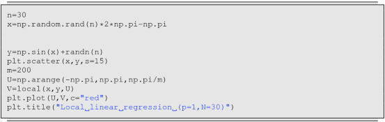
  • (b) Using the same kernel as we used in Problem 66 with p = 1, we applied x ₁, …, x _N, y ₁, …, y _N to local regression. Fill in the blanks and execute the procedure.

    

• 68. If the number of base functions is finite, the coefficient can be obtained via least squares in the same manner as linear regression. However, when the number of bases is large, such as for the smoothing spline, it is difficult to find the inverse matrix. Moreover, for example, local regression cannot be expressed by a finite number of bases. In such cases, a method called backfitting is often applied. To decompose the function into the sum of polynomial regression and local regression, we constructed the following procedure. Fill in the blanks and execute the process.