Steady-State Two-Dimensional Heat Conduction

Abstract

Previous chapters were devoted to steady-state one-dimensional systems. In this chapter, analytical solution, graphical analysis, method of analogy and numerical solutions have been presented for two-dimensional steady-state conduction heat flow through solids without heat sources. Conduction shape factor has been defined and presented for various physical systems. The presented methods have been supported by a number of numerical examples. Various techniques for the solution of nodal equations developed by the finite-difference method have been given.

Appendices

Review Questions

• 5.1 What are the various methods of solving two-dimensional heat conduction problems? Discuss their basics and limitations.

• 5.2 What are curvilinear squares?

• 5.3 Define conduction shape factor. Support your answer by considering a configuration where two-dimensional heat conduction is encountered.

• 5.4 Explain the basic principle of electrothermal analogy?

• 5.5 Explain the basic method of finite difference. What are the various methods available to obtain a solution after writing the finite-difference equations?

• 5.6 Compare relaxation and Gaussian elimination methods.

Problems

• 5.1 Using the equations of temperature distribution obtained in the analytical method for the two-dimensional heat conduction, determine the temperature at (3/4, ¼) of the long square-section rod shown in Fig. 5.41.

  Fig. 5.41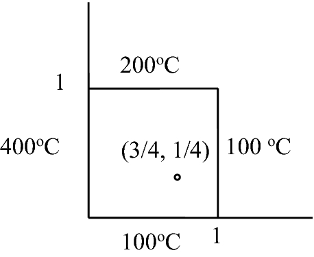

  

  Problem 5.1

  [Ans. Using the equations presented in Example 5.5, t(x, y) = 127.2°C.]

• 5.2 A cubical furnace (0.6 m side) is covered with 0.1 m thick layer of insulation [k = 0.035 W/(m K)]. If the temperature difference across the insulation is 80°C, calculate the heat loss through the layer.

  [Ans. Shape factors: S_{plane wall} = 3.6, S_edge = 0.324, S_corner = 0.015, Total shape factor, S = 25.61 m; q = 71.71 W]

• 5.3 Combustion gases at an average temperature of 1200°C flow through a 3 m long, 100 mm zero-dimensional circular section duct. In order to reduce the heat loss, the duct is covered with insulation [k = 0.05 W/(m² K)]. The insulated duct measures 250 mm × 250 mm (square in shape). Determine the heat loss for the duct if the heat transfer coefficients are h_i = 150 W/(m² K) and h₀ = 5 W/(m² K) for the duct inner and outer surfaces, respectively. T_∞ = 30°C.

  [Ans. From Case (11), Table 5.2, S = 18.98; Resistances are: R_i = 1/(2πRLh_i) = 7.074 × 10^–3, R_k = 1/kS = 1.054; and R_o = 1/(4WLh_o) = 0.0666, q = Δt/∑R = 1037.5 W.]

• 5.4 A 75 mm diameter hot fluid pipeline (surface temperature = 80°C) and a cold water pipeline 50 mm in diameter (surface temperature = 20°C) are 200 mm apart on centres in a large duct packed with glass wool insulation [k = 0.038 W/(m K)]. Calculate the heat transfer to the cold fluid for 5 m length of the pipes.

  [Ans. From Case (9), Table 5.2, S = 8.49, q = k S (80–20) = 19.36 W].

• 5.5 For a plate fin of uniform cross-section A_c along its length, show that the temperature for the tip node shown in Fig. 5.42 is given by

  Fig. 5.42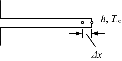

  

  Problem 5.5

  $$\left[ {h\left( {\frac{\Delta x}{k}} \right) + 1 + \frac{1}{2}\left( {m\Delta x} \right)^{2} } \right]T_{m} = \left[ {h\left( {\frac{\Delta x}{k}} \right) + \frac{1}{2}\left( {m\Delta x} \right)^{2} } \right]T_{\infty } + T_{m - 1}$$

  where m² = hP/kA_c.

  [Hint: $hA_{c} \left( {T_{\infty } - T_{m} } \right) + kA_{c} \left( {\frac{{T_{m - 1} - T_{m} }}{\Delta x}} \right) + P\frac{\Delta x}{2}h(T_{\infty } - T_{m} ) = 0$. On simplification and putting $\frac{hP}{{kA_{c} }} = m^{2}$, the result is obtained.]

• 5.6 If the end of the plate fin of Problem 5.5 is insulated, show that the temperature for the tip node is given by

  $$T_{m - 1} + \left[ {m^{2} .\frac{{(\Delta x)^{2} }}{2}} \right]T_{\infty } - \left[ {1 + m^{2} .\frac{{(\Delta x)^{2} }}{2}} \right]T_{m} = 0$$

  where m² = hP/kA_c.

  [Hint: Refer Fig. 5.43. Heat balance equation is $kA_{c} \left( {\frac{{T_{m - 1} - T_{m} }}{\Delta x}} \right) + hP\frac{\Delta x}{2}(T_{\infty } - T_{m} ) = 0$. On simplification and putting $\frac{hP}{{kA_{c} }} = m^{2}$, the result is obtained.]

  Fig. 5.43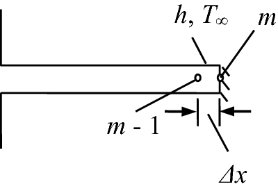

  

  Problem 5.6

• 5.7 The node (m, n) in Fig. 5.44 is situated on a boundary along which uniform heat flux $q^{\prime\prime}$ is specified. Show that in the steady-state, the node temperature is given by

  Fig. 5.44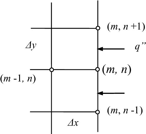

  

  Problem 5.7

  $$T_{m,n} = ({1 \mathord{\left/ {\vphantom {1 {4)}}} \right. \kern-0pt} {4)}}(T_{m,n + 1} + T_{m,n - 1} + 2T_{m - 1,n} ) + ({{q^{\prime\prime}} \mathord{\left/ {\vphantom {{q^{\prime\prime}} {2k)}}} \right. \kern-0pt} {2k)}}\Delta x$$

  Verify that the adiabatic boundary limit result deduced from the equation agrees with the corresponding result in Table 5.3.

  [Ans. The heat balance equation is

  $$k\left( {\frac{\Delta x}{2}} \right)\frac{{\left( {T_{m,n + 1} - T_{m,n} } \right)}}{\Delta y} + k\left( {\frac{\Delta x}{2}} \right)\frac{{\left( {T_{m,n - 1} - T_{m,n} } \right)}}{\Delta y} + k\left( {\Delta y} \right)\frac{{\left( {T_{m - 1,n} - T_{m,n} } \right)}}{\Delta x} + q^{{\prime \prime }} \Delta y = 0$$

  Substitution of Δx = Δy gives the desired result. For adiabatic boundary, $q^{\prime\prime} = 0$]

• 5.8 Write down the nodal equation for internal corner of a two-dimensional system with horizontal boundary insulated and vertical boundary subjected to convection heat transfer as shown in Fig. 5.45a.

  Fig. 5.45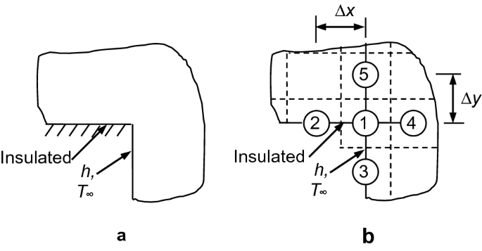

  

  Problem 5.8

  Verify that the adiabatic boundary limit result deduced from the equation agrees with the corresponding result in Table 5.3.

  [Ans. The heat balance equation for node 1 gives for unit depth, refer Fig. 5.45b,

  $$h\left( {\frac{1.\Delta y}{2}} \right)\left( {T_{\infty } - T_{1} } \right) + k\left( {\frac{1.\Delta y}{2}} \right)\frac{{\left( {T_{2} - T_{1} } \right)}}{\Delta x} + k\left( {\frac{1.\Delta x}{2}} \right)\frac{{\left( {T_{3} - T_{1} } \right)}}{\Delta y} + k\left( {1.\Delta y} \right)\frac{{\left( {T_{4} - T_{1} } \right)}}{\Delta x} + k\left( {1.\Delta x} \right)\frac{{\left( {T_{5} - T_{1} } \right)}}{\Delta y} = 0$$

  Putting Δx = Δy, we have $T_{2} + T_{3} + 2T_{4} + 2T_{5} + \left( {\frac{h\Delta y}{k}} \right)T_{\infty } - \left( {6 + \frac{h\Delta y}{k}} \right)T_{1} = 0.$ When vertical boundary is also adiabatic, put h = 0 and the result is $T_{2} + T_{3} + 2T_{4} + 2T_{5} - 6T_{1} = 0$, which is the same as for case (h) Example 5.28.]

• 5.9 Write down nodal equation for the two-dimensional steady-state conduction problem of Case (g) shown in Fig. 5.26 of Example 5.28 when the vertical boundary is insulated. Consider the dimension perpendicular to the plane of paper as b.

  [Ans. Referring to the heat balance equation of Case (g) of Example 5.28, the convective heat transfer will reduce to half and the heat balance equation for node 1 will be

  $h\left( {\frac{b\delta }{2}} \right)\left( {T_{\infty } - T_{1} } \right) + k\left( {\frac{b\delta }{2}} \right)\frac{{\left( {T_{2} - T_{1} } \right)}}{\delta } + k\left( {\frac{b\delta }{2}} \right)\frac{{\left( {T_{3} - T_{1} } \right)}}{\delta } = 0$. Simplification gives

  $T_{2} + T_{3} + \left( {\frac{h\delta }{k}} \right)T_{\infty } - \left( {2 + \frac{h\delta }{k}} \right)T_{1} = 0$. When horizontal boundary is also insulated we get result of Case (d) by putting h = 0, i.e. $T_{2} + T_{3} - 2T_{1} = 0.$]

• 5.10 Write nodal equation for the nodal point 1 on an inclined surface of a system shown in Fig. 5.46. The inclined surface is subjected to a convective heat transfer.

  Fig. 5.46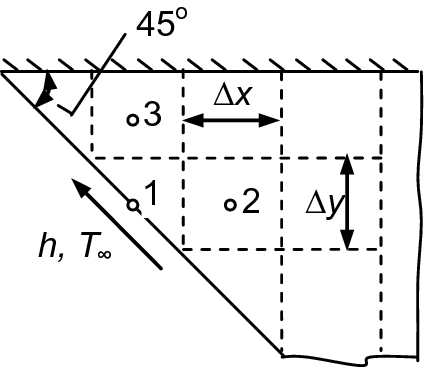

  

  Problem 5.10

  [Ans. The heat balance equation for unit depth is

  $k(\Delta y.1)\left( {\frac{{T_{2} - T_{1} }}{\Delta x}} \right) + k(\Delta x.1)\left( {\frac{{T_{3} - T_{1} }}{\Delta y}} \right) + h\left( {\sqrt {\Delta x^{2} + \Delta y^{2} } .1} \right)(T_{\infty } - T_{1} ) = 0.$ For ∆x = ∆y equation transforms to nodal equation as $T_{2} + T_{3} + \sqrt 2 \frac{h\Delta x}{k}T_{\infty } - \left( {2 + \sqrt 2 \frac{h\Delta x}{k}} \right)T_{1} = 0.$]

• 5.11 Write nodal equation for the nodal point 1 on tip of the system shown in Fig. 5.47 The inclined surface is subjected to a convective heat transfer while the horizontal surface is insulated.

  Fig. 5.47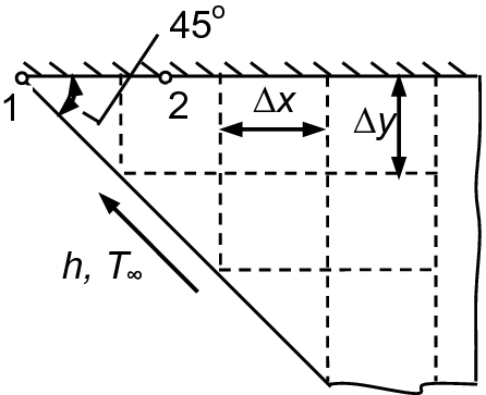

  

  Problem 5.11

  [Ans. The heat balance equation for unit depth is

  $k\left( {\frac{\Delta y}{2}.1} \right)\left( {\frac{{T_{2} - T_{1} }}{\Delta x}} \right) + h\left( {\frac{1}{2}\sqrt {\Delta x^{2} + \Delta y^{2} } .1} \right)(T_{\infty } - T_{1} ) = 0.$ For ∆x = ∆y equation transforms to nodal equation as $T_{2} + \sqrt 2 \frac{h\Delta x}{k}T_{\infty } - \left( {1 + \sqrt 2 \frac{h\Delta x}{k}} \right)T_{1} = 0.$]

• 5.12 Use the relaxation method to solve the following set of equations.

  $$500 + T_{2} + T_{4} - 4T_{1} = R_{1}$$

  (a)
  $$300 + T_{3} + T_{1} - 4T_{2} = R_{2}$$

  (b)
  $$500 + T_{4} + T_{2} - 4T_{3} = R_{3}$$

  (c)
  $$700 + T_{1} + T_{3} - 4T_{4} = R_{4}$$

  (d)

  [Ans. T₁ = 250°C, T₂ = 200°C, T₃ = 250°C, T₄ = 300°C.]