The Category of Node-and-Choice Forms, with Subcategories for Choice-Sequence Forms and Choice-Set Forms

Abstract

The literature specifies extensive-form games in many styles, but lacks a systematic way of translating across those styles. This paper is a step toward such a translation system. It defines $\mathbf {NCF}$, the category of node-and-choice forms. The category’s objects are extensive forms in essentially any style, and the category’s isomorphisms are made to accord with the literature’s small handful of ad hoc style equivalences. Further, this paper develops two full subcategories: $\mathbf {CsqF}$ for forms whose nodes are choice-sequences, and $\mathbf {CsetF}$ for forms whose nodes are choice-sets. It is shown that $\mathbf {NCF}$ is “isomorphically enclosed” in $\mathbf {CsqF}$ in the sense that each $\mathbf {NCF}$ form is isomorphic to a $\mathbf {CsqF}$ form. Similarly, it is shown that $\mathbf {CsqF}_{{{\tilde{\mathbf {a}}}}}$ is isomorphically enclosed in $\mathbf {CsetF}$ in the sense that each $\mathbf {CsqF}$ form with no-absentmindedness is isomorphic to a $\mathbf {CsetF}$ form. The converses are found to be almost immediate, and the resulting equivalences unify and simplify two ad hoc style equivalences in Kline and Luckraz (2016) and Streufert (2019). Aside from the larger agenda, this paper already makes three practical contributions. Style equivalences are made easier to derive by [1] a natural concept of isomorphic invariance and [2] the composability of isomorphic enclosures. In addition, [3] some new consequences of equivalence are systematically deduced.

The author is grateful to an anonymous reviewer for many probing questions and insights, and to Deanna Walker for valuable suggestions.

1 Introduction

1.1 Some Foundational Issues

There are many styles in which to specify an extensive-form game, and some of these styles are reviewed below in Sect. 1.2. It is widely believed that any definition or result in one style also holds in any other style. This widespread belief might be formally explored. For example, when a result in one style is translated to another style, how would we define the sense in which the translation is correct or incorrect? Also, if a new style were to be proposed, how would we define the sense in which the new style was fully or partially legitimate? This paper is part of a larger agenda to explore such foundational issues by means of category theory. Some aspects of this agenda are explored further in Sect. 1.3. Then Sects. 1.4–1.7 introduce this paper in particular.

1.2 Specification Styles

To set the stage, this subsection recalls that there are many styles in which to specify an extensive-form game. All styles must specify [a] nodes, which are variously called “histories”, “vertices”, or “states”; and [b] choices, which are variously called “actions”, “alternatives”, “labels”, or “programs”. The following paragraphs arrange the styles into five broad groups according to how the styles specify nodes and choices.

[1] Some styles specify nodes and choices abstractly without restriction. Classic examples from economics include the style of Kuhn (1953) and the style of Selten (1975). Examples from computer science and/or logic include the “labeled transition system” style¹ in Blackburn et al. (2001), p. 3, and elsewhere; the style of Shoham and Leyton-Brown (2009), p. 125; and the “epistemic process graph” style of van Benthem (2014), p. 70. A final example is the “node-and-choice” style of this paper (see Fig. 1). Because each of these styles specifies nodes and choices abstractly without restriction, each can be roughly understood to encompass all other styles as special cases.²

Fig. 1

A node-and-choice form (later called an “$\mathbf {NCF}$ form”). Player P3 selects choice $\mathsf {e}$ or choice $\mathsf {f}$ without knowing whether she is at node $\mathsf {3}$ or node $\mathsf {4}$

Fig. 2

a A choice-sequence form (later called a “$\mathbf {CsqF}$ form”). b A choice-set form (later called a “$\mathbf {CsetF}$ form”). These special kinds of node-and-choice forms are developed further in this paper

[2] Other styles specify nodes as sequences of choices. A popular example in economics is the style of Osborne and Rubinstein 1994, page 200. Examples from logic include the “logical game” style of Hodges 2013, Sect. 2, and the “epistemic forest model” style of van Benthem 2014, page 130. Examples from computer science include the “protocol” style of Parikh and Ramanujam 1985, the “history-based multi-agent structure” style of Pacuit 2007, and the “sequence-form representation” style of Shoham and Leyton-Brown 2009, page 129. A final example is the “choice-sequence” style of this paper (see Fig. 2a).

[3] Other styles specify nodes as sets of choices. Examples include the “choice-set” style of Streufert (2019) (henceforth “SE”), and also the “choice-set” style of this paper (see Fig. 2b).

There are still other possibilities. [4] Some styles specify choices as sets of nodes, as in the “simple” style of Alós-Ferrer and Ritzberger (2016), Sect. 6.3 (see Fig. 3a). [5] Other styles express both nodes and choices as sets of outcomes, as in the style of von Neumann and Morgenstern (1944), Sect. 10, and the style of Alós-Ferrer and Ritzberger (2016), Sect. 6.2 (see Fig. 3b). Possibilities [1]–[5] are arranged in a spectrum by SE (Streufert 2019), Fig. 2. Further, SE Sect. 7 explains how each possibility has its own advantages and disadvantages.

Fig. 3

In a, choices are node sets. In b, both nodes and choices are outcome sets. These special kinds of node-and-choice forms are not developed further in this paper

1.3 General Motivation

The first rigorous comparisons of specification styles have only recently appeared in Alós-Ferrer and Ritzberger (2016), Sect. 6.3, in Kline and Luckraz (2016), and in SE (whose Fig. 2 provides an overview of all these results). These contributions show, by ad hoc constructions, that the five styles in the above figures are of roughly equal generality. To be somewhat more precise, these papers argue that one style is at least as general as another style, by showing that each game³ in the first style can be reasonably mapped to a game in the second style. Then two styles are regarded as equivalent if such an argument can be made in both directions. Notice that each such argument hinges upon an ad hoc mapping linking games in one style to games in another style. Lacking is a way to compare styles that is based on a systematic way of comparing games. This paper starts to provide that systematization in a fashion that is compatible with the prior style equivalences.

Further, a larger agenda emerges, for one can hope to do more than systematically translate games from one style to games in another style. One can hope to systematically translate properties, defined for games, from one style to another. One can hope to systematically translate equilibrium concepts from one style to another. So ultimately, one can hope to systematically translate theorems from one style to another.

Such an overarching translation system promises conceptual benefits. Foremost in the author’s mind is the formal synthesis of results and questions from the many disciplines and subdisciplines which are currently studying some version of game theory. There might be much to gain because there is so much diversity. In addition, the author has been made aware of another benefit, namely, that categorical translations between games may allow for syntactic translations between the logical languages that are interpreted in those games. This would accord with the correspondence theory of van Benthem (2001), and Conradie et al. (2014).

Formal translation is a daunting task. Fortunately, category theory promises to be a powerful and natural tool. In order to gain access to this tool, the author’s current objective is to construct a category [a] whose objects are extensive-form games in any style, and [b] whose isomorphisms accord with the handful of style equivalences already in the literature. This involves three steps. The first step was Streufert (2018) (henceforth “SP”). That paper defined $\mathbf {NCP}$, which is the category of node-and-choice “preforms”, where a preform is a rooted tree with choices and information sets. The second step is the present paper. This paper defines $\mathbf {NCF}$, which is the category of node-and-choice “forms”, where a form augments a preform with players. The third step is a future paper which will augment $\mathbf {NCF}$ forms with preferences in order to define extensive-form games.

Elsewhere there is relatively little categorical work on game theory. Lapitsky (1999), and Jiménez (2014) define categories for simultaneous-move games. Machover and Terrington (2014) define a category for some cooperative games. Abramsky et al. (2000), Hyland and Ong (2000), and McCusker (2000) develop categories for some specialized games in computer science. Vannucci (2007) defines a category for extensive-form games, but every morphism merely maps a game to itself. Lastly, (Honsell et al. 2012; Abramsky and Winschel 2017; Hedges 2017; Ghani et al. 2018) define categories for various games that assume trivial information sets. Streufert (2018) and the present paper depart from the literature by considering nontrivial information sets.

1.4 This Paper’s Categorical Investments

As explained two paragraphs ago, this paper constructs a category of forms [a] whose objects are forms in any style, and [b] whose isomorphisms accord with the style equivalences already in the literature. Goals [a] and [b] are discussed in the next two paragraphs.

Section 2 introduces $\mathbf {NCF}$, which is the category of node-and-choice forms, in which both nodes and choices are specified abstractly without restriction. Thereby goal [a] is achieved. Further, one special kind of node-and-choice form is a choice-sequence form, in which nodes are choice-sequences. Correspondingly, Sect. 3 introduces $\mathbf {CsqF}$, which is the full $\mathbf {NCF}$ subcategory for choice-sequence forms. Similarly, another special kind of node-and-choice form is a choice-set form, in which nodes are choice-sets. Correspondingly, Sect. 4 introduces $\mathbf {CsetF}$, which is the full $\mathbf {NCF}$ subcategory for choice-set forms. Finally, consider again the five styles in Sect. 1.2. $\mathbf {NCF}$ itself corresponds to style [1], $\mathbf {CsqF}$ corresponds to style [2], and $\mathbf {CsetF}$ corresponds to style [3]. Left for future research are style [4] with its node-set choices, and style [5] with its outcome-set nodes and outcome-set choices. These two additional styles will correspond to two additional subcategories of $\mathbf {NCF}$, as suggested in Sect. 5.2’s discussion of future research.

To achieve goal [b], Sect. 2 defines $\mathbf {NCF}$’s morphisms in such a way that the category’s isomorphisms accord with the style equivalences in the literature. Since this paper does not build subcategories for the node-set and outcome-set styles, only two of the literature’s style equivalences remain: [i] Kline and Luckraz (2016) Theorems 1 and 2, which are essentially an equivalence between node-and-choice forms and choice-sequence forms, and [ii] SE Theorems 3.1 and 3.2, which are essentially an equivalence between (no-absentminded) choice-sequence forms and choice-set forms. As discussed earlier, each of these two equivalences is a matching pair of results, in which each result states that each form in one style can be reasonably mapped to a form in the other style. Section 3.2 proposes to strengthen each such result by requiring that each form in one style is $\mathbf {NCF}$ isomorphic to a form in the other style. This new kind of result is called an “isomorphic enclosure”, and a matching pair of isomorphic enclosures is called an “isomorphic equivalence”. Equivalence [i] accords with Corollary 3.3(b), which states that $\mathbf {NCF}$ and $\mathbf {CsqF}$ are isomorphically equivalent. Similarly, equivalence [ii] accords with Corollary 3.3(b), which states that $\mathbf {CsqF}_{{{\tilde{\mathbf {a}}}}}$ and $\mathbf {CsetF}$ are isomorphically equivalent. The paragraphs after these two corollaries provide historical context, more details, and more senses in which the two corollaries accord with literature’s equivalences [i] and [ii].

Other results show that $\mathbf {NCF}$ is pleasant in other ways. Theorem 2.3 shows that $\mathbf {NCF}$ is a well-defined category. Theorem 2.4 shows that an $\mathbf {NCF}$ isomorphism can be characterized by bijections for nodes, choices, and players. Theorem 2.7 shows that there is a forgetful functor from $\mathbf {NCF}$ to $\mathbf {NCP}$, which is SP’s category of node-and-choice preforms. In addition, various results in Sects. 2.1–2.3 show that the category interacts naturally with game-theoretic concepts like the assignment of information sets to players. Also, Sect. 2.4 shows that the properties of no-absentmindedness and perfect-information are invariant to $\mathbf {NCF}$ isomorphisms. Finally, the paragraph after Corollary 3.5 shows how the negation of isomorphic enclosure formalizes the notion that a property is truly “restrictive” and “substantial” as opposed to merely “notational”.

1.5 This Paper’s Categorical Dividends

Section 1.4 argues that $\mathbf {NCF}$ systematizes prior style equivalences and that it is a pleasant category in a variety of other ways. Also, Sects. 1.3 and 5.2 argue that $\mathbf {NCF}$ promises to be of practical importance in the larger agenda of translating game theory across styles. Further, the following three paragraphs identify three practical ways that $\mathbf {NCF}$ directly contributes to game theory.

First, isomorphic invariance is a natural and powerful concept. For example, two elementary propositions in Sect. 3.3 use isomorphic invariance to find [1] general circumstances in which one subcategory is strictly isomorphically enclosed by another and [2] general circumstances in which an isomorphic enclosure can be restricted to smaller subcategories. The latter proposition is used by Corollary 3.7(b) to easily construct an isomorphic enclosure for the proof highlighted in the next paragraph. Further, both propositions are used by Sect. 4.3 to easily derive new results about perfect-information.

Second, isomorphic enclosures can be composed (note 17). Such compositions can make it much easier to derive other isomorphic enclosures. For example, the proof of Corollary 4.3(b)’s reverse direction is just six lines long, and the third paragraph following the corollary’s proof explains how this simple argument replaces six difficult pages in SE’s proof of its Theorem 3.2. Thus the isomorphic equivalence of Corollary 4.3(b) is much easier to prove than the corresponding ad hoc equivalence of SE Theorems 3.1 and 3.2 (this was called equivalence [ii] in Sect. 1.4).

Third, isomorphic enclosures have consequences for form derivatives, and Sect. 5.1 deduces them simultaneously for all isomorphic enclosures. More specifically, each isomorphic enclosure is defined via isomorphisms, and Proposition 2.6 implies that each such isomorphism has consequences not only for form components (such as nodes, choices, and players) but also for form derivatives (such as the precedence relation among nodes, and each player’s collection of information sets). In contrast, the literature’s ad hoc style equivalences concern only form components.

1.6 Explicitness for Novice Category Theorists and Others

It is hoped that this paper can be understood by readers from economics, computer science, logic, and mathematics. Many such readers know little category theory, and these readers can benefit from the fact this paper presumes little prior knowledge of the subject. In fact, the paper’s results and proofs use just the definitions of category, isomorphism, functor, and full subcategory. These fundamental definitions can be found in the early pages of Simmons (2011), Awodey (2010), and Mac Lane (1998) (arranged in descending order of accessibility).

Because the intended audience includes novice category theorists, this paper tries to avoid the notational and conceptual shortcuts that expert category theorists use to suppress the routine details that are of no interest to them. Thus expert category theorists will find the writing unusually detailed (and perhaps also awkward, pedantic, and tedious). For example, consider Sect. 2.1’s concept of a functioned tree (T, p), which consists of a set T with an associated structure p. A category theorist would be apt to make the structure p implicit, to routinely denote a tree by T, and to routinely identify a morphism from one tree T to another tree $T{}^{\prime }$ by a function ${ \tau }{:}T\rightarrow T{}^{\prime }$. This paper keeps the structure p explicit, keeps denoting a functioned tree by (T, p), and keeps distinguishing between the function ${ \tau }{:}T\rightarrow T{}^{\prime }$ and the morphism $[(T,p),(T{}^{\prime },p'),{ \tau }]$. Such explicitness helps novice category theorists and slows expert category theorists.

More generally, because the intended audience spans several disciplines, this paper tries to avoid the specialized shortcuts that any of the disciplines use to suppress routine details. Thus, readers from almost any of the disciplines will probably find the writing uncomfortably detailed at one point or another. For example, consider the fundamental concept of a function. In particular, consider the two functions $f{:}{ \mathbb R}\rightarrow { \mathbb R}$ defined by $({ \forall }x{ \in }{ \mathbb R})$ $f(x) = \text {sin}(x)$, and $g{:}{ \mathbb R}\rightarrow [-1,1]$ defined by $({ \forall }x{ \in }{ \mathbb R})$ $g(x) = \text {sin}(x)$. A category theorist, who regards the codomain as an essential part of a function’s definition, would think $f{ \ }{ \ne }{ \ }g$ (Mac Lane 1998, p. 1). In contrast, a set theorist, who identifies a function with its graph, would think $f = g$ (Halmos 1974, pp. 30–33). Meanwhile, an economist, with applications in mind, would wonder whether understanding this issue is really worth the effort. In order to speak plainly to several disciplines at the same time, this paper will be explicit about the distinction between a function and its graph. Details are in Sect. 2.1.

1.7 Organization

Section 2 develops $\mathbf {NCF}$, the category of node-and-choice forms. Less generally, Sect. 3 develops the subcategory $\mathbf {CsqF}$ for choice-sequence forms, and Sect. 4 develops the subcategory $\mathbf {CsetF}$ for choice-set forms. Sections 3.2 and 3.3 use the context of $\mathbf {CsqF}$ to introduce the general concept of isomorphic enclosure, and to introduce general propositions about isomorphic invariance. Further, Sect. 5.1 uses parts of Sects. 3 and 4 to illustrate some general consequences of isomorphic enclosure. Finally, Sect. 5.2 discusses future research.

Although many proofs appear within the text, twelve lengthy proofs and their associated lemmas are relegated to the appendices. Appendix A concerns $\mathbf {NCF}$, Appendix B concerns $\mathbf {CsqF}$, and Appendix C concerns $\mathbf {CsetF}$.

2 The Category of Node-and-Choice Forms

2.1 Objects

Node-and-choice forms are defined and developed in terms of functions, relations, and correspondences. In accord with the last paragraph of Sect. 1.6, the next two paragraphs are explicit about these almost-standard concepts.

Let a function $f{:}X\rightarrow Y$ be a triple $(X,Y,f^{\mathsf {gr}})$, such that X and Y are sets and such that $f^{\mathsf {gr}}$ is a subset of $X{ \times }Y$ satisfying $({ \forall }x{ \in }X)({ \exists } !y{ \in }Y){ \ }(x,y){ \in }f^{\mathsf {gr}}$. The sets X, Y, and $f^{\mathsf {gr}}$ are, respectively, the domain, codomain, and graph of f. Note that many functions can share the same graph, but that only one of these functions is surjective. Thus a graph, together with the property of surjectivity, can be used to define a function.

Let a relation R between X and Y be a triple $(X,Y,R^{\mathsf {gr}})$ such that X and Y are sets and $R^{\mathsf {gr}}$ is a subset of $X{ \times }Y$. In accord with economics (Mas-Colell et al. 1995, p. 949), let a correspondence $F{:}X{ \rightrightarrows } Y$ be a triple $(X,Y,F^{\mathsf {gr}})$, such that X and Y are sets and $F^{\mathsf {gr}}$ is a subset of $X{ \times }Y$. Although relations and correspondences are formally identical, they are used in different ways. Finally, let a relation R on X be a relation of the form $(X,X,R^{\mathsf {gr}})$.

Let T be a set of elements t called nodes. As in SP Sect. 2.1 (where “SP” abbreviates Streufert 2018), a pair (T, p) is a functioned tree iff there are $t^o{ \ }{ \in }{ \ }T$ and $X{ \ }{ \subseteq }{ \ }T$ such that [T1] p is a nonempty function from $T{ \smallsetminus }{ \lbrace }t^o{ \rbrace }$ onto X and [T2] $({ \forall }t{ \in }T{ \smallsetminus }{ \lbrace }t^o{ \rbrace })({ \exists } m{ \in }{{ \mathbb N}_1})$ $p^m(t) = t^o$.⁴ Call p the (immediate) predecessor function.

A functioned tree (uniquely) determines many entities. First, it determines its root node $t^o$ and its set X of decision nodes. Second, it determines its stage function $k{:}T\rightarrow {{ \mathbb N}_0}$ by [a] $k(t^o) = 0$ and [b] $({ \forall }t{ \in }T{ \smallsetminus }{ \lbrace }t^o{ \rbrace })$ $p^{k(t)}(t) = t^o$. Third, it determines its (strict) precedence relation ${ \prec }$ on T by $({ \forall }t^1{ \in }T,t^2{ \in }T)$ $t^1{ \ }{ \prec }{ \ }t^2$ iff $({ \exists } m{ \in }{{ \mathbb N}_1})$ $t^1 = p^m(t^2)$. Relatedly, it determines its weak precedence relation ${ \preccurlyeq }$ on T by $({ \forall }t^1{ \in }T,t^2{ \in }T)$ $t^1{ \ }{ \preccurlyeq }{ \ }t^2$ iff $({ \exists } m{ \in }{{ \mathbb N}_0})$ $t^1 = p^m(t^2)$. Finally, it determines the set ${ \mathcal Z}$ of maximal chains in $(T,{ \preccurlyeq })$. This can be split into the set $\mathcal Z_{\mathsf {ft}}$ of finite maximal chains and the (possibly empty) set $\mathcal Z_{\mathsf {inft}}$ of infinite maximal chains. These derived entities and their basic properties are developed in SP Sects. 2.1 and 2.2.

Let C be a set of elements c called choices. A triple ${ \varPi }= (T,C,{ \otimes })$ is a (node-and-choice) preform (SP Sect. 3.1) iff

Call⁵$^{,}$⁶$^{,}$⁷ ${ \otimes }$ the node-and-choice operator, and let $t{ \otimes }c$ denote its value at $(t,c){ \ }{ \in }{ \ }F^{\mathsf {gr}}$. Call F the feasibility correspondence, call $t^o$ the root node, call p the immediate-predecessor function, and call ${ \mathcal H}$ the collection of information sets. In addition, let X equal $F^{-1}(C)$ (inconsequentially, SP uses $F^{-1}(C)$ rather than X). Call X the decision-node set.⁸

A node-and-choice preform ${ \varPi }$ (uniquely) determines many entities. First, it determines its F, $t^o$, p, ${ \mathcal H}$, and X, as discussed in the previous paragraph. Second, [P2] determines the functioned tree (T, p), which in turn determines k, ${ \prec }$, ${ \preccurlyeq }$, ${ \mathcal Z}$, $\mathcal Z_{\mathsf {ft}}$, and $\mathcal Z_{\mathsf {inft}}$, as discussed in the second-previous paragraph. Third, define the preform’s previous-choice function $q{:}T{ \smallsetminus }{ \lbrace }t^o{ \rbrace }\rightarrow C$ by $q^{\mathsf {gr}}= { \lbrace }(t^{\sharp },c){ \in }T{ \times }C|({ \exists } t{ \in }T)(t,c,t^{\sharp }){ \in }{ \otimes }^{\mathsf {gr}}{ \rbrace }$. All these entities and their basic properties are developed in SP Sects. 3.1 and 3.2. Among the basic properties is the convenient fact that $(p,q) = { \otimes }^{-1}$.

Let I be a set of elements i called players. A quadruple ${ \varPhi }= (I,T,(C_i)_{i{ \in }I},{ \otimes })$ is a (node-and-choice) form iff

Each $C_i$ is the set of choices that are assigned to player i. The definitions in this paragraph are new to this paper (and an earlier version, Streufert 2016).

A node-and-choice form ${ \varPhi }$ (uniquely) determines many entities. First, [F1] determines C and the preform $(T,C,{ \otimes })$, which in turn determines F, $t^o$, p, q, ${ \mathcal H}$, X, k, ${ \prec }$, ${ \preccurlyeq }$, ${ \mathcal Z}$, $\mathcal Z_{\mathsf {ft}}$, and $\mathcal Z_{\mathsf {inft}}$, as discussed in the second-previous paragraph. Second, define $(X_i)_{i{ \in }I}$ at each i by $X_i = { \cup }_{c{ \in }C_i}F^{-1}(c)$. $X_i$ is the set of decision nodes that are assigned to player i. Third, define $({ \mathcal H}_i)_{i{ \in }I}$ at each i by ${ \mathcal H}_i = { \lbrace }F^{-1}(c)|c{ \in }C_i{ \rbrace }$. ${ \mathcal H}_i$ is the collection of information sets that are assigned to player i.

Proposition 2.1

Suppose $(I,T,(C_i)_i,{ \otimes })$ is a node-and-choice form with its X, ${ \mathcal H}$, $(X_i)_{i{ \in }I}$, and $({ \mathcal H}_i)_{i{ \in }I}$. Then the following hold.

• (a) ${ \cup }_{i{ \in }I}X_i = X$ and $({ \forall }i{ \in }I,j{ \in }I{ \smallsetminus }{ \lbrace }i{ \rbrace }){ \ }X_i{ \cap }X_j = { \varnothing }$.

• (b) $({ \forall }i{ \in }I){ \ }{ \mathcal H}_i$ partitions $X_i$.

• (c) ${ \cup }_{i{ \in }I}{ \mathcal H}_i = { \mathcal H}$ and $({ \forall }i{ \in }I,j{ \in }I{ \smallsetminus }{ \lbrace }i{ \rbrace }){ \ }{ \mathcal H}_i{ \cap }{ \mathcal H}_j = { \varnothing }$. (Proof A.3.)

Here are two minor remarks. [1] A preform can be understood as a one-player form. Specifically, $(T,C,{ \otimes })$ is a preform iff $({ \lbrace }1{ \rbrace },T,(C),{ \otimes })$ is a form, where $(C_i)_i = (C)$ is taken to mean $C_1 = C$. [2] A player i in a form is said to be vacuous iff $C_i = { \varnothing }$. A vacuous player i necessarily has $X_i = { \varnothing }$ and ${ \mathcal H}_i = { \varnothing }$. Vacuous players can be convenient. For example, one can posit the existence of a chance player, and yet create a game without chance nodes by letting the chance player be vacuous.

2.2 Morphisms

A (node-and-choice) preform morphism (SP Sect. 3.3) is a quadruple ${ \alpha }= [{ \varPi },{ \varPi }{}^{\prime },{ \tau },{ \delta }]$ such that ${ \varPi }= (T,C,{ \otimes })$ and ${ \varPi }{}^{\prime } = (T{}^{\prime },C{}^{\prime },{ \otimes }{}^{\prime })$ are preforms,

SP Propositions 3.3 and 3.4 give two characterizations of preform morphisms which feel more category-theoretic. A (node-and-choice) form morphism is a quintuple ${ \beta }= [{ \varPhi },{ \varPhi }{}^{\prime },{ \iota },{ \tau },{ \delta }]$ s.t. ${ \varPhi }= (I,T,(C_i)_{i{ \in }I},{ \otimes })$ and ${ \varPhi }{}^{\prime } = (I{}^{\prime },T{}^{\prime },(C{}^{\prime }_{i{}^{\prime }})_{i{}^{\prime }{ \in }I{}^{\prime }},{ \otimes }{}^{\prime })$ are forms,

The first paragraph of Proposition 2.2 rearranges the definition of a morphism. Meanwhile, the second and third paragraphs concern the many derivatives which can be constructed, via Sect. 2.1, from the source and target forms. Parts (k) and (m) are new, while the remainder are obtained by combining [FM1] with various SP results for preforms and trees.

Proposition 2.2

Suppose ${ \varPhi }= (I,T,(C_i)_{i{ \in }I},{ \otimes })$ and ${ \varPhi }{}^{\prime } = (I{}^{\prime },T{}^{\prime },(C{}^{\prime }_{i{}^{\prime }})_{i{}^{\prime }{ \in }I{}^{\prime }},{ \otimes }{}^{\prime })$ are forms. Let $C = { \cup }_{i{ \in }I}C_i$ and $C{}^{\prime } = { \cup }_{i{}^{\prime }{ \in }I{}^{\prime }}C{}^{\prime }_{i{}^{\prime }}$. Then $[{ \varPhi },{ \varPhi }{}^{\prime },{ \iota },{ \tau },{ \delta }]$ is a morphism iff the following hold.

• (a) ${ \iota }\,{:}\,I\,\rightarrow \,I{}^{\prime }$ .

• (b) ${ \tau }\,{:}\,T\,\rightarrow \,T{}^{\prime }$ .

• (c) ${ \delta }\,{:}\,C\,\rightarrow \,C{}^{\prime }$ .

• (d) $({ \forall }i{ \in }I){ \ }{ \delta }(C_i){ \ }{ \subseteq }{ \ }C{}^{\prime }_{{ \iota }(i)}$.

• (e) ${ \lbrace }\,({ \tau }(t),{ \delta }(c),{ \tau }(t^{\sharp }))\,|\,(t,c,t^{\sharp }){ \in }{ \otimes }^{\mathsf {gr}}\,{ \rbrace }{ \ }{ \subseteq }{ \ }{ \otimes }{}^{\prime \,\mathsf {gr}}$.

Further, suppose $[{ \varPhi },{ \varPhi }{}^{\prime },{ \iota },{ \tau },{ \delta }]$ is a morphism. Let ${ \varPi }= (T,C,{ \otimes })$ and ${ \varPi }{}^{\prime } = (T{}^{\prime },C{}^{\prime },{ \otimes }{}^{\prime })$. Also, derive F, $t^o$, p, q, X, $(X_i)_{i{ \in }I}$, ${ \mathcal H}$, and $({ \mathcal H}_i)_{i{ \in }I}$ from ${ \varPi }$ and ${ \varPhi }$. Also, derive $F{}^{\prime }$, $t^{\prime o}$, $p{}^{\prime }$, $q{}^{\prime }$, $X{}^{\prime }$, $(X{}^{\prime }_{i{}^{\prime }})_{i{}^{\prime }{ \in }I{}^{\prime }}$, ${ \mathcal H}{}^{\prime }$, and $({ \mathcal H}{}^{\prime }_{i{}^{\prime }})_{i{}^{\prime }{ \in }I{}^{\prime }}$ from ${ \varPi }{}^{\prime }$ and ${ \varPhi }{}^{\prime }$. Then the following hold.

• (f) ${ \lbrace }\,({ \tau }(t),{ \delta }(c))\,|\,(t,c){ \in }F^{\mathsf {gr}}\,{ \rbrace }{ \ }{ \subseteq }{ \ }F{}^{\prime \,\mathsf {gr}}$.

• (g) $t^{\prime o}{ \ }{ \preccurlyeq }{}^{\prime }{ \ }{ \tau }(t^o)$.

• (h) ${ \lbrace }\,({ \tau }(t^{\sharp }),{ \tau }(t))\,|\,(t^{\sharp },t){ \in }p^{\mathsf {gr}}\,{ \rbrace }{ \ }{ \subseteq }{ \ }p{}^{\prime \,\mathsf {gr}}$.

• (i) ${ \lbrace }\,({ \tau }(t^{\sharp }),{ \delta }(c))\,|\,(t^{\sharp },c){ \in }q^{\mathsf {gr}}\,{ \rbrace }{ \ }{ \subseteq }{ \ }q{}^{\prime \,\mathsf {gr}}$.

• (j) ${ \tau }(X){ \ }{ \subseteq }{ \ }X{}^{\prime }$.

• (k) $({ \forall }i{ \in }I){ \ }{ \tau }(X_i){ \ }{ \subseteq }{ \ }X{}^{\prime }_{{ \iota }(i)}$.

• (l) $({ \forall }H{ \in }{ \mathcal H})({ \exists } H{}^{\prime }{ \in }{ \mathcal H}{}^{\prime }){ \ }{ \tau }(H){ \ }{ \subseteq }{ \ }H{}^{\prime }$.

• (m) $({ \forall }i{ \in }I,H{ \in }{ \mathcal H}_i)({ \exists } H{}^{\prime }{ \in }{ \mathcal H}{}^{\prime }_{{ \iota }(i)}){ \ }{ \tau }(H){ \ }{ \subseteq }{ \ }H{}^{\prime }$.

Finally, derive k, ${ \prec }$, ${ \preccurlyeq }$, $\mathcal Z_{\mathsf {ft}}$, and $\mathcal Z_{\mathsf {inft}}$ from (T, p). Also, derive $k{}^{\prime }$, ${ \prec }{}^{\prime }$, ${ \preccurlyeq }{}^{\prime }$, $\mathcal Z_{\mathsf {ft}}{}^{\prime }$, and $\mathcal Z_{\mathsf {inft}}{}^{\prime }$ from $(T{}^{\prime },p{}^{\prime })$. Then the following hold.

• (n) $({ \forall }t{ \in }T){ \ }k{}^{\prime }({ \tau }(t)) = k(t) + k{}^{\prime }({ \tau }(t^o))$.

• (o) ${ \lbrace }\,({ \tau }(t^1),{ \tau }(t^2))\,|\,(t^1,t^2){ \in }{ \prec }^{\mathsf {gr}}\,{ \rbrace }{ \ }{ \subseteq }{ \ }{ \prec }{}^{\prime \,\mathsf {gr}}$.

• (p) ${ \lbrace }\,({ \tau }(t^1),{ \tau }(t^2))\,|\,(t^1,t^2){ \in }{ \preccurlyeq }^{\mathsf {gr}}\,{ \rbrace }{ \ }{ \subseteq }{ \ }{ \preccurlyeq }{}^{\prime \,\mathsf {gr}}$.

• (q) $({ \forall }Z{ \in } \mathcal Z_{\mathsf {ft}})({ \exists } Z{}^{\prime }{ \in } \mathcal Z_{\mathsf {ft}}{}^{\prime }{ \cup }\mathcal Z_{\mathsf {inft}}{}^{\prime }){ \ }{ \tau }(Z){ \ }{ \subseteq }{ \ }Z{}^{\prime }$.

• (r) $({ \forall }Z{ \in }\mathcal Z_{\mathsf {inft}})({ \exists } Z{}^{\prime }{ \in }\mathcal Z_{\mathsf {inft}}{}^{\prime }){ \ }{ \tau }(Z){ \ }{ \subseteq }{ \ }Z{}^{\prime }$. (Proof A.4.)

2.3 The Category $\mathbf {NCF}$

This paragraph and Theorem 2.3 define the category $\mathbf {NCF}$, which is called the category of node-and-choice forms. Let an object be a (node-and-choice) form ${ \varPhi }= (I,T,(C_i)_{i{ \in }I},{ \otimes })$. Let an arrow be a (node-and-choice) form morphism ${ \beta }= [{ \varPhi },{ \varPhi }{}^{\prime },{ \iota },{ \tau },{ \delta }]$. Let source, target, identity, and composition be

$$\begin{aligned} \begin{array}{c} { \beta }^\mathsf {src}= [{ \varPhi },{ \varPhi }{}^{\prime },{ \iota },{ \tau },{ \delta }]^\mathsf {src}= { \varPhi }, \nonumber \\ { \beta }^\mathsf {trg}= [{ \varPhi },{ \varPhi }{}^{\prime },{ \iota },{ \tau },{ \delta }]^\mathsf {trg}= { \varPhi }{}^{\prime }, \nonumber \\ \mathsf {id}_{ \varPhi }= \mathsf {id}_{(I,T,(C_i)_{i{ \in }I},{ \otimes })} = [{ \varPhi },{ \varPhi },\mathsf {id}_{I},\mathsf {id}_{T},\mathsf {id}_{{ \cup }_{i{ \in }I}C_i}],{ \ }\text {and} \nonumber \\ { \beta }{}^{\prime }{ \circ }{ \beta }= [{ \varPhi }{}^{\prime },{ \varPhi }{}^{\prime \prime },{ \iota }{}^{\prime },{ \tau }{}^{\prime },{ \delta }{}^{\prime }]{ \circ }[{ \varPhi },{ \varPhi }{}^{\prime },{ \iota },{ \tau },{ \delta }] = [{ \varPhi },{ \varPhi }{}^{\prime \prime },{ \iota }{}^{\prime }{ \circ }{ \iota },{ \tau }{}^{\prime }{ \circ }{ \tau },{ \delta }{}^{\prime }{ \circ }{ \delta }],\, \nonumber \end{array} \end{aligned}$$

where $\mathsf {id}_I$, $\mathsf {id}_T$, and $\mathsf {id}_{{ \cup }_{i{ \in }I}C_i}$ are identities in $\mathbf {Set}$.

Theorem 2.3

$\mathbf {NCF}$ is a category. (Proof A.5.)

Theorem 2.4

Suppose ${ \beta }= [{ \varPhi },{ \varPhi }{}^{\prime },{ \iota },{ \tau },{ \delta }]$ is a morphism. Then (a) ${ \beta }$ is an isomorphism iff ${ \iota }$, ${ \tau }$, and ${ \delta }$ are bijections. Further (b) if ${ \beta }$ is an isomorphism, then ${ \beta }^{-1} = [{ \varPhi }{}^{\prime },{ \varPhi },{ \iota }^{-1},{ \tau }^{-1},{ \delta }^{-1}]$. (Proof A.7.)

Corollary 2.5

Suppose $[{ \varPhi },{ \varPhi }{}^{\prime },{ \iota },{ \tau },{ \delta }]$ is a morphism. Let ${ \varPi }$ be the preform in ${ \varPhi }$, and let ${ \varPi }{}^{\prime }$ be the preform in ${ \varPhi }{}^{\prime }$. Then $[{ \varPhi },{ \varPhi }{}^{\prime },{ \iota },{ \tau },{ \delta }]$ is an isomorphism iff [1] $[{ \varPi },{ \varPi }{}^{\prime },{ \tau },{ \delta }]$ is a preform isomorphism and [2] ${ \iota }$ is a bijection.

Proof

Note $[{ \varPi },{ \varPi }{}^{\prime },{ \tau },{ \delta }]$ is a preform morphism by [FM1] for $[{ \varPhi },{ \varPhi }{}^{\prime },{ \iota },{ \tau },{ \delta }]$. Thus SP Theorem 3.7(a) shows that [1] is equivalent to the bijectivity of ${ \tau }$ and ${ \delta }$. Therefore [1] and [2] together are equivalent to the bijectivity of ${ \iota }$, ${ \tau }$, and ${ \delta }$. By Theorem 2.4(a), this is equivalent to $[{ \varPhi },{ \varPhi }{}^{\prime },{ \iota },{ \tau },{ \delta }]$ being an isomorphism. $\square$

Proposition 2.6 organizes some⁹ of the consequences of a form isomorphism. The proposition’s first paragraph concerns form components, while the second and third paragraphs concern form derivatives. Consequences (a)–(c) repeat the forward direction of Theorem 2.4(a). Consequences (d), (k), and (m) are new, while the remainder are obtained by combining the forward direction of Corollary 2.5 with SP results about preforms and trees. The entire proposition is comparable to Proposition 2.2 for morphisms, and Sect. 5.1 will discuss how the proposition contributes directly to game theory.

To address a minor technical issue, note that many of the proposition’s consequences are formulated by restricting functions. In each case, the codomain of the restriction is defined so that the restriction is surjective. Two other minor technical issues are discussed in notes 10 and 11.

Proposition 2.6

Suppose $[{ \varPhi },{ \varPhi }{}^{\prime },{ \iota },{ \tau },{ \delta }]$ is an isomorphism, where ${ \varPhi }= (I,T,$ $(C_i)_{i{ \in }I},{ \otimes })$ and ${ \varPhi }{}^{\prime } = (I{}^{\prime },T{}^{\prime },(C{}^{\prime }_{i{}^{\prime }})_{i{}^{\prime }{ \in }I{}^{\prime }},{ \otimes }{}^{\prime })$. Let $C = { \cup }_{i{ \in }I}C_i$ and $C{}^{\prime } = { \cup }_{i{}^{\prime }{ \in }I{}^{\prime }}C{}^{\prime }_{i{}^{\prime }}$. Then the following hold.

• (a) ${ \iota }$ is a bijection from I onto $I{}^{\prime }$.

• (b) ${ \tau }$ is a bijection from T onto $T{}^{\prime }$.

• (c) ${ \delta }$ is a bijection from C onto $C{}^{\prime }$.

• (d) $({ \forall }i{ \in }I){ \ }{ \delta }|_{C_i}$ is a bijection from $C_i$ onto $C{}^{\prime }_{{ \iota }(i)}$.¹⁰

• (e) $({ \tau },{ \delta },{ \tau })|_{{ \otimes }^{\mathsf {gr}}}$ is a bijection from ${ \otimes }^{\mathsf {gr}}$ onto ${ \otimes }{}^{\prime \,\mathsf {gr}}$.

Further, let ${ \varPi }= (T,C,{ \otimes })$ and ${ \varPi }{}^{\prime } = (T{}^{\prime },C{}^{\prime },{ \otimes }{}^{\prime })$. Also, derive F, $t^o$, p, q, X, $(X_i)_{i{ \in }I}$, ${ \mathcal H}$, and $({ \mathcal H}_i)_{i{ \in }I}$ from ${ \varPi }$ and ${ \varPhi }$. Also, derive $F{}^{\prime }$, $t^{\prime o}$, $p{}^{\prime }$, $q{}^{\prime }$, $X{}^{\prime }$, $(X{}^{\prime }_{i{}^{\prime }})_{i{}^{\prime }{ \in }I{}^{\prime }}$, ${ \mathcal H}{}^{\prime }$, and $({ \mathcal H}{}^{\prime }_{i{}^{\prime }})_{i{}^{\prime }{ \in }I{}^{\prime }}$ from ${ \varPi }{}^{\prime }$ and ${ \varPhi }{}^{\prime }$. Then the following hold.

• (f) $({ \tau },{ \delta })|_{F^{\mathsf {gr}}}$ is a bijection from $F^{\mathsf {gr}}$ onto $F{}^{\prime \,\mathsf {gr}}$.

• (g) ${ \tau }(t^o) = t^{\prime o}$.

• (h) $({ \tau },{ \tau })|_{p^{\mathsf {gr}}}$ is a bijection from $p^{\mathsf {gr}}$ onto $p{}^{\prime \,\mathsf {gr}}$.

• (i) $({ \tau },{ \delta })|_{q^{\mathsf {gr}}}$ is a bijection from $q^{\mathsf {gr}}$ onto $q{}^{\prime \,\mathsf {gr}}$.

• (j) ${ \tau }|_X$ is a bijection from X onto $X{}^{\prime }$.

• (k) $({ \forall }i{ \in }I){ \ }{ \tau }|_{X_i}$ is a bijection from $X_i$ onto $X{}^{\prime }_{{ \iota }(i)}$.$^{10}$

• (l) ${ \tau }|_{{ \mathcal H}}$ is a bijection from ${ \mathcal H}$ onto ${ \mathcal H}{}^{\prime }$.¹¹

• (m) $({ \forall }i{ \in }I){ \ }{ \tau }|_{{ \mathcal H}_i}$ is a bijection from ${ \mathcal H}_i$ onto ${ \mathcal H}{}^{\prime }_{{ \iota }(i)}$.$^{10}$ $^{,}$ $^{11}$

Finally, derive k, ${ \prec }$, ${ \preccurlyeq }$, ${ \mathcal Z}$, $\mathcal Z_{\mathsf {ft}}$, and $\mathcal Z_{\mathsf {inft}}$ from (T, p). Also, derive $k{}^{\prime }$, ${ \prec }{}^{\prime }$, ${ \preccurlyeq }{}^{\prime }$, ${ \mathcal Z}{}^{\prime }$, $\mathcal Z_{\mathsf {ft}}{}^{\prime }$, $\mathcal Z_{\mathsf {inft}}{}^{\prime }$ from $(T{}^{\prime },p{}^{\prime })$. Then the following hold.

• (n) $({ \forall }t{ \in }T) { \ }k{}^{\prime }({ \tau }(t)) = k(t)$.

• (o) $({ \tau },{ \tau })|_{{ \prec }^{\mathsf {gr}}}$ is a bijection from ${ \prec }^{\mathsf {gr}}$ onto ${ \prec }{}^{\prime \,\mathsf {gr}}$.

• (p) $({ \tau },{ \tau })|_{{ \preccurlyeq }^{\mathsf {gr}}}$ is a bijection from ${ \preccurlyeq }^{\mathsf {gr}}$ onto ${ \preccurlyeq }{}^{\prime \,\mathsf {gr}}$.

• (q) ${ \tau }|_{ \mathcal Z_{\mathsf {ft}}}$ is a bijection from $\mathcal Z_{\mathsf {ft}}$ onto $\mathcal Z_{\mathsf {ft}}{}^{\prime }$.$^{11}$

• (r) ${ \tau }|_{\mathcal Z_{\mathsf {inft}}}$ is a bijection from $\mathcal Z_{\mathsf {inft}}$ onto $\mathcal Z_{\mathsf {inft}}$.$^{11}$

• (s) ${ \tau }|_{{ \mathcal Z}}$ is a bijection from ${ \mathcal Z}$ onto ${ \mathcal Z}{}^{\prime }$.$^{11}$ (Proof A.9.)

As already noted, the definition of a form incorporates a preform, and the definition of a form morphism incorporates a preform morphism. Correspondingly, Theorem 2.7 shows there is a “forgetful” functor $\mathsf {P}$ from $\mathbf {NCF}$ to $\mathbf {NCP}$, where $\mathbf {NCP}$ is SP’s category of node-and-choice preforms.¹²

Theorem 2.7

Define $\mathsf {P}$ from $\mathbf {NCF}$ to $\mathbf {NCP}$ by

$$\begin{aligned} \begin{array}{c} \mathsf {P_0}{ \ }:{ \ }(I,T,(C_i)_{i{ \in }I},{ \otimes }){ \ }\mapsto (T,{ \cup }_{i{ \in }I}C_i,{ \otimes }){ \ }\text {and} \quad \quad \\ \quad \mathsf {P_1}{ \ }:{ \ }[{ \varPhi },{ \varPhi }{}^{\prime },{ \iota },{ \tau },{ \delta }]{ \ }\mapsto { \ }[\mathsf {P_0}({ \varPhi }),\mathsf {P_0}({ \varPhi }{}^{\prime }),{ \tau },{ \delta }].\nonumber \end{array} \end{aligned}$$

Then $\mathsf {P}$ is a well-defined functor. (Proof A.10.)

2.4 No-Absentmindedness and Perfect-Information

Consider an arbitrary category $\mathbf {Z}$, and a property which is defined for the objects of $\mathbf {Z}$. The property is said to be isomorphically invariant iff, for each object, the object satisfies the property iff all of its isomorphs satisfy the property. This section explores two isomorphically invariant properties: [1] no-absentmindedness and [2] perfect-information. Both properties restrict information sets.

No-absentmindedness is a standard property which is widely regarded as being very weak (see, for example, Alós-Ferrer and Ritzberger 2016, Sect. 4.2.3). To define this property in $\mathbf {NCP}$, consider an $\mathbf {NCP}$ preform with its ${ \prec }$ and ${ \mathcal H}$. Then the preform is said to have no-absentmindedness iff .¹³ Further, consider an $\mathbf {NCF}$ form with its preform. Then the form is said to have no-absentmindedness iff its preform has no-absentmindedness.

Proposition 2.8

(a$^o$) If $[{ \varPi },{ \varPi }{}^{\prime },{ \tau },{ \delta }]$ is an $\mathbf {NCP}$ morphism and ${ \varPi }{}^{\prime }$ has no-absentmindedness, then ${ \varPi }$ has no-absentmindedness. (a) No-absentmindedness is isomorphically invariant in $\mathbf {NCP}$. (b$^o$) If $[{ \varPhi },{ \varPhi }{}^{\prime },{ \iota },{ \tau },{ \delta }]$ is an $\mathbf {NCF}$ morphism and ${ \varPhi }{}^{\prime }$ has no-absentmindedness, then ${ \varPhi }$ has no-absentmindedness. (b) No-absentmindedness is isomorphically invariant in $\mathbf {NCF}$. (Proof A.11.)

Let $\mathbf {NCP}_{{{\tilde{\mathbf {a}}}}}$ be the full subcategory of $\mathbf {NCP}$ whose objects are preforms with no-absentmindedness. (Subscripts are being used for isomorphically invariant properties.) Similarly, let $\mathbf {NCF}_{{{\tilde{\mathbf {a}}}}}$ be the full subcategory of $\mathbf {NCF}$ whose objects are forms with no-absentmindedness. No-absentmindedness will appear again in Sect. 3.3.

Perfect-information is another standard property. It is restrictive, and at the same time, there are many interesting games which satisfy it (see, for example, Osborne and Rubinstein 1994 Part II). As in SP Sect. 3.5, an $\mathbf {NCP}$ preform, with its collection ${ \mathcal H}$ of information sets H, is said to have perfect-information iff $({ \forall }H{ \in }{ \mathcal H})$ $|H| = 1$. Perfect-information is strictly stronger than no-absentmindedness.¹⁴$^{,}$¹⁵ Further, an $\mathbf {NCF}$ form is said to have perfect-information iff the form’s preform has perfect-information. (In spite of Proposition 2.9, the existence of a morphism does not lead to any logical relationship between the source’s perfect-information and the target’s perfect-information. Thus there is no “Proposition 2.9(a$^o$)” to mimic Proposition 2.8(a$^o$).)

Proposition 2.9

(a) Perfect-information is isomorphically invariant in $\mathbf {NCP}$. (b) Perfect-information is isomorphically invariant in $\mathbf {NCF}$. (Proof A.12.)

Let $\mathbf {NCP_p}$ be the full subcategory of $\mathbf {NCP}$ whose objects are preforms with perfect-information. (The subscript ${}_{\tilde{\mathbf {a}}{\mathbf {p}}}$ would be equivalent to the subscript $\mathbf {_p}$, because no-absentmindedness is implied by perfect-information, as shown in note 14.) Further, let $\mathbf {NCF_p}$ be the full subcategory of $\mathbf {NCF}$ whose objects are forms with perfect-information. Perfect-information will appear again in Sect. 4.3.

3 The Subcategory of Choice-Sequence Forms

3.1 Objects

Let a (finite) sequence be the graph of a function from ${ \lbrace }1,2, \ldots \,m{ \rbrace }$ for some nonnegative integer m (to be clear, the empty sequence¹⁶ with empty domain is admitted by $m = 0$). Thus this paper regards a sequence as a set of ordered pairs. For example, $t^* = { \lbrace }(1,{\mathsf {g}}),$ $(2,{\mathsf {f}}),$ $(3,{\mathsf {f}}){ \rbrace }$ is a sequence with domain ${ \lbrace }1,2,3{ \rbrace }$. An alternative notation for the same entity is $t^* = (\mathsf {g,f,f})$. Yet another is $t^* = (t^*_n)^3_{n=1}$ where $t^*_1 = {\mathsf {g}}$ and $t^*_2 = t^*_3 = {\mathsf {f}}$.

Let the length of a sequence t be |t|. For instance, the length of the example sequence is $|t^*|$ $=$ $|{ \lbrace }(1,{\mathsf {g}}),(2,{\mathsf {f}}),(3,{\mathsf {f}}){ \rbrace }|$ $= 3$, which is consistent with the observation that $(2,{\mathsf {f}})$ ${ \ne }$ $(3,{\mathsf {f}})$. Note that the length of the empty sequence ${ \lbrace }{ \rbrace }$ is $|{ \lbrace }{ \rbrace }| = 0$. Next, let the range of a sequence t be $R(t) = { \lbrace }\,t_n\,|\,n{ \in }{ \lbrace }1,2, \ldots \,|t|{ \rbrace }\,{ \rbrace }$. For instance, the range of the example sequence is $R(t^*) = { \lbrace }\,t^*_n\,|\,n{ \in }{ \lbrace }1,2,3{ \rbrace }\,{ \rbrace }= { \lbrace }{\mathsf {g}},{\mathsf {f}},{\mathsf {f}}{ \rbrace }= { \lbrace }{\mathsf {g}},{\mathsf {f}}{ \rbrace }$. Note that the range of the empty sequence ${ \lbrace }{ \rbrace }$ is $R({ \lbrace }{ \rbrace }) = { \varnothing }$.

Let the concatenation $t{ \oplus }s$ of two sequences t and s be ${ \lbrace }(1,t_1),$ $\ldots$ $(|t|,t_{|t|}),$ $(|t|{+}1,s_1),$ $\ldots$ $(|t|{+}|s|,s_{|s|}){ \rbrace }$. Thus the concatenation of a sequence $t = (t_1,t_2,\ldots \,t_{|t|})$ with a one-element sequence (c) is $t{ \oplus }(c) = (t_1,t_2,\ldots \,t_{|t|},c)$. Next, for any sequence t and any ${ \ell }{ \ }{ \in }{ \ }{ \lbrace }0,1,2,\ldots \,|t|{ \rbrace }$, let $_1t_{ \ell }$ denote the initial segment $(t_1,t_2,\ldots \,t_{ \ell })$. Thus for any sequence t, $_1t_0 = { \lbrace }{ \rbrace }$.

A choice-sequence $\mathbf {NCP}$ preform is an $\mathbf {NCP}$ preform $(T,C,{ \otimes })$ such that

Let $\mathbf {CsqP}$ be the full subcategory of $\mathbf {NCP}$ whose objects are choice-sequence preforms. Proposition 3.1 lists some of the special properties of $\mathbf {CsqP}$ preforms. Incidentally, property (i) and assumption [Csq1] together imply that each node in a $\mathbf {CsqP}$ preform is actually a choice sequence, as the terminology suggests.

Proposition 3.1

Suppose $(T,C,{ \otimes })$ is a $\mathbf {CsqP}$ preform. Derive its F, $t^o$, p, q, k, ${ \prec }$, and ${ \preccurlyeq }$. Then the following hold.

• (a) $t^o = { \lbrace }{ \rbrace }$.

• (b) $({ \forall }t^{\sharp }{ \in }T{ \smallsetminus }{ \lbrace }{ \lbrace }{ \rbrace }{ \rbrace }){ \ }p(t^{\sharp }) = {_1t^{\sharp }_{|t^{\sharp }|-1}}\,\text {and}{ \ }q(t^{\sharp }) = t^{\sharp }_{|t^{\sharp }|}$.

• (c) ${ \otimes }^{\mathsf {gr}}= { \lbrace }{ \ }(t,c,t^{\sharp }){ \in }T{ \times }C{ \times }T{ \ }|{ \ }t{ \oplus }(c){=}t^{\sharp }{ \ }{ \rbrace }$.

• (d) $F^{\mathsf {gr}}= { \lbrace }{ \ }(t,c){ \in }T{ \times }C{ \ }|{ \ }t{ \oplus }(c){ \in }T{ \ }{ \rbrace }$.

• (e) $({ \forall }t{ \in }T,m{ \in }{ \lbrace }0,1,...\,|t|{ \rbrace }){ \ }p^m(t) = {_1t_{|t|-m}}$.

• (f) $({ \forall }t{ \in }T)$ $k(t) = |t|$.

• (g) $({ \forall }t{ \in }T){ \ }t = (q{ \circ }p^{|t|-{ \ell }}(t))^{|t|}_{{ \ell }=1}$.

• (h) $C = { \cup }_{t{ \in }T}R(t)$.

• (i) $({ \forall }t^A{ \in }T,t^B{ \in }T)$ $t^A{ \ }{ \prec }{ \ }t^B$ iff $(|t^A|\,{<}\,|t^B|{ \ }\text {and}{ \ }t^A\,{=}\,{_1t^B_{|t^A|}})$.

• (j) $({ \forall }t^A{ \in }T,t^B{ \in }T)$ $t^A{ \ }{ \preccurlyeq }{ \ }t^B$ iff $(|t^A|\,{ \le }\,|t^B|{ \ }\text {and}{ \ }t^A\,{=}\,{_1t^B_{|t^A|}})$. (Proof B.1.)

Finally, let a choice-sequence $\mathbf {NCF}$ form be an $\mathbf {NCF}$ form whose preform is a $\mathbf {CsqP}$ preform. Then let $\mathbf {CsqF}$ be the full subcategory of $\mathbf {NCF}$ whose objects are choice-sequence $\mathbf {NCF}$ forms.

3.2 Isomorphic Enclosure

Consider two full subcategories $\mathbf {A}$ and $\mathbf {B}$ of some overarching category $\mathbf {Z}$. Say that $\mathbf {A}$ is isomorphically enclosed in $\mathbf {B}$ (in symbols, $\mathbf {A}$ $\mathop \rightarrow \limits _{\cdot }$ $\mathbf {B}$) iff every object of $\mathbf {A}$ is isomorphic to an object of $\mathbf {B}$. Note that $\mathbf {A}$ ${\mathop \rightarrow \limits _{\cdot }}$ $\mathbf {B}$ concerns not only the subcategories $\mathbf {A}$ and $\mathbf {B}$ but also, implicitly, the overarching category $\mathbf {Z}$ within which isomorphisms are defined. Further note that isomorphic enclosures can be composed in the sense that $\mathbf {A}$ ${\mathop \rightarrow \limits _{\cdot }}$ $\mathbf {B}$ and $\mathbf {B}$ ${\mathop \rightarrow \limits _{\cdot }}$ $\mathbf {C}$ imply $\mathbf {A}$ ${\mathop \rightarrow \limits _{\cdot }}$ $\mathbf {C}$.¹⁷ Finally, let ${{\mathbf {A}}{ \ }\mathop {\leftrightarrow } \limits _{\cdot }{ \ }{\mathbf {B}}}$ mean that both ${{\mathbf {A}}{ \ }\mathop \rightarrow \limits _{\cdot }{ \ }{\mathbf {B}}}$ and ${{\mathbf {A}}{ \ }\mathop {\leftarrow } \limits _{\cdot }{ \ }{\mathbf {B}}}$ hold. Call ${\mathop {\leftrightarrow } \limits _{\cdot }}$ isomorphic equivalence. Isomorphic equivalence implies the standard categorical concept of equivalence in Mac Lane (1998) p. 18.

Theorem 3.2

(a) $\mathbf {NCP}$ ${\mathop \rightarrow \limits _{\cdot }}$ $\mathbf {CsqP}$. In particular, suppose ${ \varPi }= (T,C,{ \otimes })$ is an $\mathbf {NCP}$ preform with its p, q, and k. Define $\bar{T}= { \lbrace }\,(q{ \circ }p^{k(t)-{ \ell }}(t))^{k(t)}_{{ \ell }=1}\,|\,t{ \in }T\,{ \rbrace }$, define $\bar{{ \tau }}{:}T\rightarrow \bar{T}$ by $\bar{{ \tau }}(t) = (q{ \circ }p^{k(t)-{ \ell }}(t))^{k(t)}_{{ \ell }=1}$, and define $\bar{{ \otimes }}$ by surjectivity and $\bar{{ \otimes }}^{\mathsf {gr}}= { \lbrace }\,(\bar{{ \tau }}(t),c,\bar{{ \tau }}(t^{\sharp }))\,|\,(t,c,t^{\sharp }){ \in }{ \otimes }^{\mathsf {gr}}\,{ \rbrace }$. Then $\bar{{ \varPi }} = (\bar{T},C,\bar{{ \otimes }})$ is an $\mathbf {CsqP}$ preform, $\bar{{ \tau }}$ is a bijection, and $[{ \varPi },\bar{{ \varPi }},\bar{{ \tau }},\mathsf {id}_C]$ is an $\mathbf {NCP}$ isomorphism. (b) $\mathbf {NCF}$ ${\mathop \rightarrow \limits _{\cdot }}$ $\mathbf {CsqF}$. In particular, suppose ${ \varPhi }= (I,T,(C_i)_{i{ \in }I},{ \otimes })$ is an $\mathbf {NCF}$ form. Define $\bar{T}$, $\bar{{ \tau }}$, and $\bar{{ \otimes }}$ as in part (a). Then $\bar{{ \varPhi }} = (I,\bar{T},(C_i)_{i{ \in }I},\bar{{ \otimes }})$ is a $\mathbf {CsqF}$ form and $[{ \varPhi },\bar{{ \varPhi }},\mathsf {id}_I,\bar{{ \tau }},\mathsf {id}_{{ \cup }_{i{ \in }I}C_i}]$ is an $\mathbf {NCF}$ isomorphism. (Proof B.3.)¹⁸

Corollary 3.3

(a) $\mathbf {NCP}$ ${\mathop {\leftrightarrow } \limits _{\cdot }}$ $\mathbf {CsqP}$. (b) $\mathbf {NCF}$ ${\mathop {\leftrightarrow } \limits _{\cdot }}$ $\mathbf {CsqF}$.

Proof

(a). $\mathbf {NCP}$ ${\mathop \rightarrow \limits _{\cdot }}$ $\mathbf {CsqP}$ by Theorem 3.2(a). Conversely, each $\mathbf {CsqP}$ preform is an $\mathbf {NCP}$ preform by definition. (b). This is very similar to (a). Change “preform” to “form”, $\mathbf {P}$ to $\mathbf {F}$, and (a) to (b). $\square$

This equivalence has a long history. In the more distant past, it was informally understood that game trees could be specified in terms of either [i] a collection of nodes and a collection of edges or [ii] a collection of sequences. Harris (1985) p. 617 provides an example of this informal understanding. Specification style [i] uses the nomenclature of graph theory (e.g., Tutte 1984), and style-[i] trees were the basis on which Kuhn (1953) and Selten (1975) built game forms. Later, style-[ii] trees became the basis on which Osborne and Rubinstein (1994) built game forms.

Kline and Luckraz (2016)¹⁹ (henceforth “KL16”) develop this equivalence by a pair of theorems. In recognition of the above authors, they call style-[i] forms “KS forms” and call style-[ii] forms “OR forms”. Then, one of their theorems (their Theorem 2) shows that a KS form can be derived from each OR form, while the other theorem (their Theorem 1) shows that each KS form can be mapped to an OR form.²⁰ These two theorems are depicted by the two arrows in Fig. 4a. The arrows are dashed to convey that the equivalence is ad hoc.

Fig. 4

a The ad hoc equivalence of Kline and Luckraz (2016). b The isomorphic equivalence of Corollary 3.3(b). T = Theorem. C = Corollary

Corollary 3.3(b) develops the equivalence further. Style-[i] forms are written as $\mathbf {NCF}$ forms, and style-[ii] forms are written as $\mathbf {CsqF}$ forms. Corollary 3.3(b) is then a pair of results: one half (the very easy half) shows that an $\mathbf {NCF}$ form is isomorphic to each $\mathbf {CsqF}$ form, while the other half (Theorem 3.2) shows that each $\mathbf {NCF}$ form is isomorphic to a $\mathbf {CsqF}$ form. Thus the corollary’s isomorphic equivalence strengthens the KL16 equivalence by introducing isomorphisms.

There are further senses in which the corollary’s isomorphic equivalence accords with the KL16 equivalence. In the backward direction, KL16 Theorem 2 is appealing because the nodes in the constructed KS form are identical to the sequences in the given OR form. This is possible because KS nodes admit OR sequences as special cases. Nonetheless KL16 Theorem 2 is nontrivial because KS forms do not admit OR forms as special cases. Here the analogous result is cleaner: $\mathbf {NCF}$ forms have been defined so that $\mathbf {NCF}$ forms admit $\mathbf {CsqF}$ forms as special cases. In the forward direction, KL16 Theorem 1 is made appealing by KL16 Lemma 2, which shows that there is a bijection ${ \alpha }$ from the “vertex histories” in the given KS form to the nodes in the constructed OR form. That bijection is closely related to Theorem 3.2’s bijection $\bar{{ \tau }}$, which maps from the nodes of the given $\mathbf {NCF}$ form to the nodes in the constructed $\mathbf {CsqF}$ form.

3.3 More About No-Absentmindedness

3.3.1. Proposition 3.4 describes a general situation in which one subcategory strictly isomorphically encloses another. In the proposition, w and s are two properties defined for the objects of $\mathbf {Z}$. Further, $w{ \ }\Leftarrow \not {\Rightarrow }{ \ }s$ means that w is strictly weaker than s. In other words, $w{ \ }\Leftarrow \not {\Rightarrow }{ \ }s$ means that [a] each object of $\mathbf {Z}$ satisfies w if it satisfies s, and [b] there is an object of $\mathbf {Z}$ that satisfies w but not s. Corollary 3.5 applies Proposition 3.4 to the nonvacuous property of no-absentmindedness.

Proposition 3.4

Suppose w and s are properties defined for the objects of $\mathbf {Z}$, and that s is isomorphically invariant. Let $\mathbf {Z_w}$ be the full subcategory of $\mathbf {Z}$ whose objects satisfy w, and let $\mathbf {Z_s}$ be the full subcategory of $\mathbf {Z}$ whose objects satisfy s. Then $w{ \ }\Leftarrow \not {\Rightarrow }{ \ }s$ implies $\mathbf {Z_w}$ $\mathop {\leftarrow } \limits _{\cdot }\!{{\not \!\!\mathop \rightarrow \limits _{\cdot }}}$ $\mathbf {Z_s}$.

Proof

Suppose $w{ \ }\Leftarrow \not {\Rightarrow }{ \ }s$. To see $\mathbf {Z_w}$ ${\mathop {\leftarrow } \limits _{\cdot }}$ $\mathbf {Z_s}$, take an object of $\mathbf {Z_s}$. Since $w{ \ }{\Leftarrow }{ \ }s$, the object is also an object of $\mathbf {Z_w}$. Thus (trivially) the object is isomorphic to an object of $\mathbf {Z_w}$. To see $\mathbf {Z_w}$ ${{\not \!\!\mathop \rightarrow \limits _{\cdot }}}$ $\mathbf {Z_s}$, note the assumption $w{ \ }\Leftarrow \not {\Rightarrow }{ \ }s$ implies that there is an object of $\mathbf {Z}$ that satisfies w and violates s. Thus there is an object of $\mathbf {Z_w}$ that violates s. Thus since s is isomorphically invariant, this object does not have an isomorph that satisfies s. Thus the object does not have an isomorph in $\mathbf {Z_s}$. $\square$

Corollary 3.5

(a) $\mathbf {NCP}$ $\mathop {\leftarrow } \limits _{\cdot }\!{{\not \!\!\mathop \rightarrow \limits _{\cdot }}}$ $\mathbf {NCP}_{{{\tilde{\mathbf {a}}}}}$. (b) $\mathbf {NCF}$ $\mathop {\leftarrow } \limits _{\cdot }\!{{\not \!\!\mathop \rightarrow \limits _{\cdot }}}$ $\mathbf {NCF}_{{{\tilde{\mathbf {a}}}}}$.

Proof

(a). Consider Proposition 3.4 at $\mathbf {Z}$ equal to $\mathbf {NCP}$, when w is the vacuous property satisfied by all objects of $\mathbf {NCP}$, and s is the property of no-absentmindedness. No-absentmindedness is invariant by Proposition 2.8(a). Further the vacuous property is strictly weaker than no-absentmindedness because there exists an absentminded preform (recall note 13). Thus Proposition 3.4 implies that $\mathbf {NCP_w}$ = $\mathbf {NCP}$ strictly isomorphically encloses $\mathbf {NCP_s}$ = $\mathbf {NCP}_{{{\tilde{\mathbf {a}}}}}$. (b). This is very similar to (a). Change “preform” to “form”, $\mathbf {P}$ to $\mathbf {F}$, and (a) to (b). $\square$

To better interpret Corollary 3.5, recall Theorem 3.2(b) which states $\mathbf {NCF}$ ${\mathop \rightarrow \limits _{\cdot }}$ $\mathbf {CsqF}$. Formally, this means each $\mathbf {NCF}$ form is isomorphic to a $\mathbf {CsqF}$ form. This can be interpreted to mean that the property of having choice-sequence nodes is not “restrictive”. In contrast, Corollary 3.5(b) implies $\mathbf {NCF}$ ${\not \mathop \rightarrow \limits _{\cdot }}$ $\mathbf {NCF}_{{{\tilde{\mathbf {a}}}}}$. Formally, this means there is at least one $\mathbf {NCF}$ form (such as the one in note 13) that is not isomorphic to an $\mathbf {NCF}_{{{\tilde{\mathbf {a}}}}}$ form. This can be interpreted to mean that the property of no-absentmindedness is “restrictive”. Informally, the first result states that choice-sequence-ness is “purely notational”. In contrast, the second result states that no-absentmindedness is “substantial”, “significant”, and “real”, and that it “limits the range of decision processes and social interactions that can be modelled”. The categorical concept of isomorphic enclosure (${\mathop \rightarrow \limits _{\cdot }}$) serves to formalize and to standardize these important terms. Note that both an isomorphic enclosure, and the negation of an isomorphic enclosure, are meaningful.

3.3.2. Next, Proposition 3.6 shows that an isomorphic enclosure can be restricted by any isomorphically invariant property. Corollary 3.7 uses this result to restrict Corollary 3.3 by no-absentmindedness. Corollary 3.7 will in turn be used in the remarkably quick proof of Corollary 4.3.

Proposition 3.6

Suppose that $\mathbf {A}$ and $\mathbf {B}$ are full subcategories of $\mathbf {Z}$, and that w is an isomorphically invariant property defined for the objects of $\mathbf {Z}$. Let $\mathbf {A_w}$ be the full subcategory of $\mathbf {A}$ whose objects satisfy w, and let $\mathbf {B_w}$ be the full subcategory of $\mathbf {B}$ whose objects satisfy w. Then $\mathbf {A}$ ${\mathop \rightarrow \limits _{\cdot }}$ $\mathbf {B}$ implies $\mathbf {A_w}$ ${\mathop \rightarrow \limits _{\cdot }}$ $\mathbf {B_w}$.

Proof

Suppose $\mathbf {A}$ ${\mathop \rightarrow \limits _{\cdot }}$ $\mathbf {B}$. To show $\mathbf {A_w}$ $\mathop \rightarrow \limits _{\cdot }$ $\mathbf {B_w}$, take an object of $\mathbf {A_w}$. Then [1] the object is an object of $\mathbf {A}$ and [2] the object satisfies w. By [1] and $\mathbf {A}$ $\mathop \rightarrow \limits _{\cdot }$ $\mathbf {B}$, the object has an isomorph in $\mathbf {B}$. By [2] and the isomorphic invariance of w, the isomorph satisfies w. The conclusions of the previous two sentences imply that the isomorph is in $\mathbf {B_w}$. $\square$

Corollary 3.7

(a) $\mathbf {NCP}_{{{\tilde{\mathbf {a}}}}}$ $\mathop {\leftrightarrow } \limits _{\cdot }$ $\mathbf {CsqP}_{{{\tilde{\mathbf {a}}}}}$. (b) $\mathbf {NCF}_{{{\tilde{\mathbf {a}}}}}$ $\mathop {\leftrightarrow } \limits _{\cdot }$ $\mathbf {CsqF}_{{{\tilde{\mathbf {a}}}}}$.

Proof

(a) follows from Corollary 3.3(a), Proposition 3.6, and Proposition 2.8(a). (b) is very similar to (a). Just change (a) to (b). $\square$

Fig. 5

Half of the previous figure, augmented with some results about no-absentmindedness. C = Corollary

3.3.3. Finally, Corollary 3.8 could be proved by mimicking the proof of Corollary 3.5, in which case Proposition 3.4 would be employed once for part (a) at $\mathbf {Z}$ = $\mathbf {CsqP}$, and again for part (b) at $\mathbf {Z}$ = $\mathbf {CsqF}$. Instead, Corollary 3.8 is proved by composing isomorphic enclosures (note 17), and the proof of the corollary’s part (b) is illustrated by Fig. 5. Both proof techniques are straightforward, and a more interesting example of composition will soon appear in the proof of Corollary 4.3.

Corollary 3.8

(a) $\mathbf {CsqP}$ $\mathop {\leftarrow } \limits _{\cdot }\!{{\not \!\!\mathop \rightarrow \limits _{\cdot }}}$ $\mathbf {CsqP}_{{{\tilde{\mathbf {a}}}}}$. (b) $\mathbf {CsqF}$ $\mathop {\leftarrow } \limits _{\cdot }\!{{\not \!\!\mathop \rightarrow \limits _{\cdot }}}$ $\mathbf {CsqF}_{{{\tilde{\mathbf {a}}}}}$.

Proof

(a). This is very similar to (b). Change $\mathbf {F}$ to $\mathbf {P}$, and (b) to (a). (b). To see $\mathbf {CsqF}$ $\mathop {\leftarrow } \limits _{\cdot }$ $\mathbf {CsqF}_{{{\tilde{\mathbf {a}}}}}$, note that $\mathbf {CsqF}$ $\mathop {\leftarrow } \limits _{\cdot }$ $\mathbf {NCF}$ $\mathop {\leftarrow } \limits _{\cdot }$ $\mathbf {NCF}_{{{\tilde{\mathbf {a}}}}}$ $\mathop {\leftarrow } \limits _{\cdot }$ $\mathbf {CsqF}_{{{\tilde{\mathbf {a}}}}}$ by, respectively, Corollary 3.3(b), Corollary 3.5(b), and Corollary 3.7(b). To see $\mathbf {CsqF}$ ${\not \!\!\mathop \rightarrow \limits _{\cdot }}$ $\mathbf {CsqF}_{{{\tilde{\mathbf {a}}}}}$, suppose it were. Then $\mathbf {NCF}$ $\mathop \rightarrow \limits _{\cdot }$ $\mathbf {CsqF}$ $\mathop \rightarrow \limits _{\cdot }$ $\mathbf {CsqF}_{{{\tilde{\mathbf {a}}}}}$ $\mathop \rightarrow \limits _{\cdot }$ $\mathbf {NCF}_{{{\tilde{\mathbf {a}}}}}$ by, respectively, Corollary 3.3(b), the supposition of the previous sentence, and Corollary 3.7(b). This contradicts Corollary 3.5(b), which states that $\mathbf {NCF}$ ${\not \!\!\mathop \rightarrow \limits _{\cdot }}$ $\mathbf {NCF}_{{{\tilde{\mathbf {a}}}}}$. $\square$

4 The Subcategory of Choice-Set Forms

4.1 Objects

Let a choice-set $\mathbf {NCP}$ preform be an $\mathbf {NCP}$ preform $(T,C,{ \otimes })$ such that

Then let $\mathbf {CsetP}$ be the full subcategory of $\mathbf {NCP}$ whose objects are choice-set $\mathbf {NCP}$ preforms. Proposition 4.1 lists some of the special properties of $\mathbf {CsetP}$ preforms.²¹ Incidentally, property (f) and assumption [Cset1] together imply that each node in a $\mathbf {CsetP}$ preform is actually a choice set, in accord with the terminology. More significantly, property (g) shows that every $\mathbf {CsetP}$ preform has no-absentmindedness. In this sense the combination of [Cset1] and [Cset2] is restrictive.

Proposition 4.1

Suppose $(T,C,{ \otimes })$ is a $\mathbf {CsetP}$ preform with its F, $t^o$, p, q, k, ${ \prec }$, ${ \preccurlyeq }$, and ${ \mathcal H}$. Then the following hold.

• (a) $t^o = { \lbrace }{ \rbrace }$.

• (b) $({ \forall }t^{\sharp }{ \in }T{ \smallsetminus }{ \lbrace }{ \lbrace }{ \rbrace }{ \rbrace })$ $q(t^{\sharp }){ \ }{ \notin }{ \ }p(t^{\sharp })$ and $p(t^{\sharp }){ \cup }{ \lbrace }q(t^{\sharp }){ \rbrace }= t^{\sharp }$.

• (c) $({ \forall }t{ \in }T)$ $k(t) = |t|$.

• (d) $({ \forall }t{ \in }T,m{ \in }{ \lbrace }0,1,...\,|t|{ \rbrace })$ $p^m(t)\,{ \subseteq }\,t$ and $t{ \smallsetminus }p^m(t)$ $=$ ${ \lbrace }\,q{ \circ }p^n(t)\,|\,\!$ $m{>}n{ \ge }0\,{ \rbrace }$.

• (e) $({ \forall }t{ \in }T){ \ }t = { \lbrace }\,q{ \circ }p^n(t)\,|\,|t|{>}n{ \ge }0\,{ \rbrace }$.

• (f) $C = { \cup }T$.

• (g) $(T,C,{ \otimes })$ has no-absentmindedness.

• (h) $({ \forall }t{ \in }T,H{ \in }{ \mathcal H})$ $|t{ \cap }F(H)|{ \ }{ \le }{ \ }1$.

• (i) $({ \forall }t^A{ \in }T,t^B{ \in }T)$ $t^A{ \ }{ \subseteq }{ \ }t^B$ implies $t^A = p^{|t^B|-|t^A|}(t^B)$.

• (j) $({ \forall }t^A{ \in }T,t^B{ \in }T){ \ }t^A{ \ }{ \prec }{ \ }t^B$ iff $t^A{ \ }{ \subset }{ \ }t^B$.

• (k) $({ \forall }t^A{ \in }T,t^B{ \in }T){ \ }t^A{ \ }{ \preccurlyeq }{ \ }t^B$ iff $t^A{ \ }{ \subseteq }{ \ }t^B$.

• (l) ${ \otimes }^{\mathsf {gr}}= { \lbrace }{ \ }(t,c,t^{\sharp }){ \in }T{ \times }C{ \times }T{ \ }|{ \ }c{ \notin }t,{ \ }t{ \cup }{ \lbrace }c{ \rbrace }{=}t^{\sharp }{ \ }{ \rbrace }$.²²

• (m) $F^{\mathsf {gr}}= { \lbrace }{ \ }(t,c){ \in }T{ \times }C{ \ }|{ \ }c{ \notin }t,{ \ }t{ \cup }{ \lbrace }c{ \rbrace }{ \in }T{ \ }{ \rbrace }$. (Proof C.2.)

Finally, let a choice-set $\mathbf {NCF}$ form be an $\mathbf {NCF}$ form whose preform is a $\mathbf {CsetP}$ preform. Then let $\mathbf {CsetF}$ be the full subcategory of $\mathbf {NCF}$ whose objects are choice-set $\mathbf {NCF}$ forms.

4.2 Isomorphic Enclosure

Theorem 4.2

(a) $\mathbf {CsqP}_{{{\tilde{\mathbf {a}}}}}$ $\mathop \rightarrow \limits _{\cdot }$ $\mathbf {CsetP}$. In particular, suppose $\bar{{ \varPi }} = (\bar{T},{\bar{C}},\bar{{ \otimes }})$ is a $\mathbf {CsqP}_{{{\tilde{\mathbf {a}}}}}$ preform. Define $T = R(\bar{T})$, and define ${ \otimes }$ by surjectivity and ${ \otimes }^{\mathsf {gr}}= { \lbrace }\,(R(\bar{t}),\bar{c},R(\bar{t}^{\sharp }))\,|\,(\bar{t},\bar{c},\bar{t}^{\sharp }){ \in }\bar{{ \otimes }}^{\mathsf {gr}}\,{ \rbrace }$. Then ${ \varPi }= (T,{\bar{C}},{ \otimes })$ is a $\mathbf {CsetP}$ preform, $R|_{\bar{T}}$ is a bijection, and $[\bar{{ \varPi }},{ \varPi },R|_{\bar{T}},\mathsf {id}_{{\bar{C}}}]$ is an $\mathbf {NCP}$ isomorphism. (b) $\mathbf {CsqF}_{{{\tilde{\mathbf {a}}}}}$ $\mathop \rightarrow \limits _{\cdot }$ $\mathbf {CsetF}$. In particular, suppose $\bar{{ \varPhi }} = ({\bar{I}},\bar{T},({\bar{C}}_{\bar{i}})_{{\bar{i}}{ \in }{\bar{I}}},\bar{{ \otimes }})$ is a $\mathbf {CsqF}_{{{\tilde{\mathbf {a}}}}}$ form. Define T and ${ \otimes }$ as in part (a). Then ${ \varPhi }= ({\bar{I}},T,({\bar{C}}_{\bar{i}})_{{\bar{i}}{ \in }{\bar{I}}},{ \otimes })$ is a $\mathbf {CsetF}$ form and $[\bar{{ \varPhi }},{ \varPhi },\mathsf {id}_{\bar{I}},R|_{\bar{T}},\mathsf {id}_{{ \cup }_{{\bar{i}}{ \in }{\bar{I}}}{\bar{C}}_{\bar{i}}}]$ is an $\mathbf {NCF}$ isomorphism. (Proof C.3.)

Corollary 4.3

(a) $\mathbf {CsqP}_{{{\tilde{\mathbf {a}}}}}$ $\mathop {\leftrightarrow } \limits _{\cdot }$ $\mathbf {CsetP}$. (b) $\mathbf {CsqF}_{{{\tilde{\mathbf {a}}}}}$ $\mathop {\leftrightarrow } \limits _{\cdot }$ $\mathbf {CsetF}$.

Proof

(a). This is very similar to (b). Change “form” to “preform”, $\mathbf {F}$ to $\mathbf {P}$, (b) to (a), and the last phrase to “because it has no-absentmindedness by Proposition 4.1(g)”.

(b). Theorem 4.2(b) shows $\mathbf {CsqF}_{{{\tilde{\mathbf {a}}}}}$ $\mathop \rightarrow \limits _{\cdot }$ $\mathbf {CsetF}$. Thus it remains to show $\mathbf {CsqF}_{{{\tilde{\mathbf {a}}}}}$ $\mathop {\leftarrow } \limits _{\cdot }$ $\mathbf {CsetF}$. Since isomorphic enclosures can be composed, it suffices to show [1] $\mathbf {CsetF}$ $\mathop \rightarrow \limits _{\cdot }$ $\mathbf {NCF}_{{{\tilde{\mathbf {a}}}}}$ and [2] $\mathbf {NCF}_{{{\tilde{\mathbf {a}}}}}$ $\mathop \rightarrow \limits _{\cdot }$ $\mathbf {CsqF}_{{{\tilde{\mathbf {a}}}}}$. [2] is the forward direction of Corollary 3.7(b). [1] holds simply because any $\mathbf {CsetF}$ form is a $\mathbf {NCF}_{{{\tilde{\mathbf {a}}}}}$ form. To see this, take a $\mathbf {CsetF}$ form. It is an $\mathbf {NCF}$ form by construction. It has no-absentmindedness because its preform has no-absentmindedness by Proposition 4.1(g). $\square$

Fig. 6

a An ad hoc equivalence from SE. b The previous figure, augmented with Corollary 4.3(b) and its proof. T $=$ Theorem. C $=$ Corollary

Corollary 4.3(b) is analogous to an ad hoc style equivalence in SE. There, a pair of results argues that no-absentminded OR forms (“OR$\bar{\text {a}}$ forms” in this subsection) are equivalent to SE-choice-set forms (“SEcs forms” in this subsection). One of the results (SE Theorem 3.2) shows that an OR$\bar{\text {a}}$ form can be reasonably derived from each SEcs form, and the other result (SE Theorem 3.1) shows that each OR$\bar{\text {a}}$ form can be reasonably mapped to an SEcs form. These two theorems are depicted by the two dashed arrows in Fig. 6a.

Corollary 4.3(b) strengthens this equivalence. $\mathbf {CsqF}_{{{\tilde{\mathbf {a}}}}}$ forms are like OR$\bar{\text {a}}$ forms in that both specify nodes as choice-sequences, and $\mathbf {CsetF}$ forms are like SEcs forms in that both specify nodes as choice-sets. Then, Corollary 4.3(b)’s isomorphic equivalence is a matching pair of results: one half (labelled “easy” in Fig. 6b) shows that a $\mathbf {CsqF}_{{{\tilde{\mathbf {a}}}}}$ form is isomorphic to each $\mathbf {CsetF}$ form, while the other half (Theorem 4.2) shows that each $\mathbf {CsqF}_{{{\tilde{\mathbf {a}}}}}$ form is isomorphic to a $\mathbf {CsetF}$ form. Thus Corollary 4.3(b) strengthens the SE equivalence by introducing isomorphisms.²³

Corollary 4.3(b)’s proof highlights how useful it is to compose isomorphic enclosures. In particular, consider the reverse direction of Corollary 4.3(b), which is $\mathbf {CsqF}_{{{\tilde{\mathbf {a}}}}}$ $\mathop {\leftarrow } \limits _{\cdot }$ $\mathbf {CsetF}$ in Fig. 6b, and compare it with SE Theorem 3.2, which is OR$\bar{\text {a}}$ $\dashleftarrow$ SEcs in Fig. 6a. The lemmas and proof for SE Theorem 3.2 span six difficult pages. In contrast, the reverse direction of Corollary 4.3(b) is proved in six lines by composing an easily-proved enclosure ($\mathbf {CsetF}$ $\mathop \rightarrow \limits _{\cdot }$ $\mathbf {NCF}_{{{\tilde{\mathbf {a}}}}}$ in part [1] of proof) with a previously-proved enclosure ($\mathbf {NCF}_{{{\tilde{\mathbf {a}}}}}$ $\mathop \rightarrow \limits _{\cdot }$ $\mathbf {CsqF}_{{{\tilde{\mathbf {a}}}}}$ from the forward half of Corollary 3.7(b)). Figure 6b shows this composition as the curved arrow followed by the forward direction of Corollary 3.7(b).

4.3 More About Perfect-Information

Corollaries 4.4 and 4.5 are additional applications of Sect. 3.3’s general propositions using isomorphic invariance.

Corollary 4.4

(a) $\mathbf {NCP}_{{{\tilde{\mathbf {a}}}}}$ $\mathop {\leftarrow } \limits _{\cdot }\!{{\not \!\!\mathop \rightarrow \limits _{\cdot }}}$ $\mathbf {NCP_p}$. (b) $\mathbf {NCF}_{{{\tilde{\mathbf {a}}}}}$ $\mathop {\leftarrow } \limits _{\cdot }\!{{\not \!\!\mathop \rightarrow \limits _{\cdot }}}$ $\mathbf {NCF_p}$.

Proof

(a). Consider Proposition 3.4 at $\mathbf {Z}$ equal to $\mathbf {NCP}$, when w is the property of no-absentmindedness ${{\tilde{\mathbf {a}}}}$, and s is the property of perfect-information p. Perfect-information is isomorphically invariant by Proposition 2.9(a). Further no-absentmindedness is strictly weaker than perfect-information by notes 14 and 15. Thus Proposition 3.4 implies that $\mathbf {NCP}_{{{\tilde{\mathbf {a}}}}}$ strictly isomorphically encloses $\mathbf {NCP_p}$. (b). This is very similar to (a). Change $\mathbf {P}$ to $\mathbf {F}$, and (a) to (b). $\square$

Corollary 4.5

(a) $\mathbf {NCP_p}$ $\mathop {\leftrightarrow } \limits _{\cdot }$ $\mathbf {CsqP_p}$ $\mathop {\leftrightarrow } \limits _{\cdot }$ $\mathbf {CsetP_p}$. (b) $\mathbf {NCF_p}$ $\mathop {\leftrightarrow } \limits _{\cdot }$ $\mathbf {CsqF_p}$ $\mathop {\leftrightarrow } \limits _{\cdot }$ $\mathbf {CsetF_p}$.

Proof

(a). Corollary 3.7(a) and Corollary 4.3(a) imply $\mathbf {NCP}_{{{\tilde{\mathbf {a}}}}}$ $\mathop {\leftrightarrow } \limits _{\cdot }$ $\mathbf {CsqP}_{{{\tilde{\mathbf {a}}}}}$ $\mathop {\leftrightarrow } \limits _{\cdot }$ $\mathbf {CsetP}$. Thus, Propositions 3.6 and 2.9(a) imply that $\mathbf {NCP}_{{{{\tilde{\mathbf {a}}}}} \mathbf{p}}$ $\mathop {\leftrightarrow } \limits _{\cdot }$ $\mathbf {CsqP}_{{{{\tilde{\mathbf {a}}}}} \mathbf{p}}$ $\mathop {\leftrightarrow } \limits _{\cdot }$ $\mathbf {CsetP_p}$, where $\mathbf {NCP}_{{{{\tilde{\mathbf {a}}}}} \mathbf{p}}$ is the full subcategory of $\mathbf {NCP}$ consisting of those objects that satisfy both no-absentmindedness and perfect-information, and where similarly $\mathbf {CsqP}_{{{{\tilde{\mathbf {a}}}}} \mathbf{p}}$ is the full subcategory of $\mathbf {CsqP}$ consisting of those objects that satisfy both no-absentmindedness and perfect-information. Since no-absentmindedness is weaker than perfect-information (note 14), $\mathbf {NCP}_{{{{\tilde{\mathbf {a}}}}} \mathbf{p}}$ = $\mathbf {NCP_p}$ and $\mathbf {CsqP}_{{{{\tilde{\mathbf {a}}}}} \mathbf{p}}$ = $\mathbf {CsqP_p}$. (b). This is very similar to (a). Change $\mathbf {P}$ to $\mathbf {F}$, and (a) to (b). $\square$

Fig. 7

Most of the previous figure, augmented with some results about perfect-information. C $=$ Corollary

Incidentally, since isomorphic equivalence implies categorical equivalence, Corollary 4.5(a) implies $\mathbf {NCP_p}$, $\mathbf {CsqP_p}$, and $\mathbf {CsetP_p}$ are categorically equivalent. Further, SP Theorem 3.13 and Corollary 3.14 show that $\mathbf {NCP_p}$, $\mathbf {Tree}$, and $\mathbf {Grph_{ca}}$ are categorically equivalent, where $\mathbf {Tree}$ is the category of functioned trees which SP uses in its development of $\mathbf {NCP}$, and where $\mathbf {Grph_{ca}}$ is the full subcategory of $\mathbf {Grph}$ whose objects are converging arborescences. Thus, $\mathbf {NCP_p}$, $\mathbf {CsqP_p}$, $\mathbf {CsetP_p}$, $\mathbf {Tree}$, and $\mathbf {Grph_{ca}}$ are categorically equivalent.

Figure 7’s arrow diagram illustrates most of the isomorphic-enclosure results from Sects. 3.2 and following. In addition, the diagram has some unlabelled arrows. They are derived by composing arrows as in the proof of Corollary 3.8. Many diagonal arrows could be similarly derived.

5 Further Remarks

5.1 Deducing Consequences from an Isomorphic Enclosure

Consider this paper’s first isomorphic enclosure. Theorem 3.2 shows that each $\mathbf {NCF}$ form ${ \varPhi }$ is isomorphic to a $\mathbf {CsqF}$ form $\bar{{ \varPhi }}$ by means of an isomorphism which transforms nodes via the bijection $\bar{{ \tau }}$. Proposition 2.6 deduces many consequences from such an isomorphism. For example, its part (o) implies that $({ \forall }t^1{ \in }T,t^2{ \in }T)$ $t^1{ \ }{ \prec }{ \ }t^2$ iff $\bar{{ \tau }}(t^1){ \ }\bar{{ \prec }}{ \ }\bar{{ \tau }}(t^2)$, where T is the node set of ${ \varPhi }$, ${ \prec }$ is derived from ${ \varPhi }$, and $\bar{{ \prec }}$ is derived from $\bar{{ \varPhi }}$. Although such consequences about form derivatives like ${ \prec }$ and $\bar{{ \prec }}$ are tantalizingly natural, the consequences about form derivatives in Proposition 2.6(f)–(s) take about 10 pages to prove. That work is important because such consequences are fundamental to drawing more conclusions from the isomorphic enclosure of $\mathbf {NCF}$ in $\mathbf {CsqF}$.

As Sect. 3.2 explained, the isomorphic enclosure of $\mathbf {NCF}$ in $\mathbf {CsqF}$ is analogous to KL16 Theorem 1. No consequences about form derivatives have been deduced from that ad hoc theorem, and an analog of Proposition 2.6(f)–(s) would likely require about 10 pages to prove. Moreover, like KL16 Theorem 1, no consequences about form derivatives have been deduced from KL16 Theorem 2 or from SE Theorems 3.1 and 3.2. Each of these ad hoc theorems has its own formulation, so deriving analogs of Proposition 2.6(f)–(s) for the three of them would likely require another $3{ \times }10 = 30$ pages.

In contrast, Proposition 2.6(f)–(s) applies not only to the isomorphic enclosure of $\mathbf {NCF}$ in $\mathbf {CsqF}$. It applies to any isomorphic enclosure. Thus it applies to all the arrows in Fig. 7, as well as to all isomorphic enclosures in the future.

5.2 Future Research

As discussed in Sect. 1.3, this paper is part of a larger agenda to translate game theory across specification styles. In this larger context, isomorphic enclosures can be seen as a way to translate form components from one style to another, and on the basis of these isomorphic enclosures, Proposition 2.6(f)–(s) (discussed just above) can be seen as a way of translating form derivatives from one style to another.

The results of this paper wait to be expanded in three orthogonal directions.

[1] There is more to translate beyond forms and their derivatives. This would include properties that forms might satisfy, and theorems that might relate these properties to one another. (This paper makes some limited progress in this direction by exploring the isomorphically invariant properties of no-absentmindedness and perfect-information, and by identifying some special properties of $\mathbf {CsqF}$ forms and $\mathbf {CsetF}$ forms via Propositions 3.1 and 4.1.) Expanding in this direction would correspond to expanding the three substantive sections of this paper.

[2] This paper concerns only three styles: $\mathbf {NCF}$, $\mathbf {CsqF}$, and $\mathbf {CsetF}$. There are other styles to explore, including the two neglected styles mentioned at the start of this paper, namely, the “node-set” style of Alós-Ferrer and Ritzberger (2016), Sect. 6.3, and the “outcome-set” style of von Neumann and Morgenstern (1944), Alós-Ferrer and Ritzberger (2016) Sect. 6.2. Expanding in this direction will require defining new $\mathbf {NCF}$ subcategories for “node-set” forms and “outcome-set” forms, and will correspond to adding, to the present paper, two new sections for the two new subcategories.

[3] This paper concerns only forms, which need to be augmented with preferences in order to define games. At the higher level of games, many more issues emerge. To return to [1], there is more to translate, including equilibrium concepts and the theorems which might relate one equilibrium concept to another. To return to [2], there will be more than five styles because there are alternative ways to specify preferences over the same form. Expanding in this third direction will require building a new category for games which incorporates this paper’s category for forms.

Appendices

Appendix A: $\mathbf {NCF}$

Lemma A.1

Suppose $(T,C,{ \otimes })$ is an $\mathbf {NCP}$ preform with its F, $t^o$, p, q, and ${ \mathcal H}$. Then the following hold.

• (a) $|T|{ \ }{ \ge }{ \ }2$, $|C|{ \ }{ \ge }{ \ }1$, $|{ \otimes }^{\mathsf {gr}}|{ \ }{ \ge }{ \ }1$.

• (b) $({ \forall }H{ \in }{ \mathcal H},c{ \in }C)$ $c{ \ }{ \in }{ \ }F(H)$ iff $F^{-1}(c) = H$.

• (c) $({ \forall }H{ \in }{ \mathcal H},t^{\sharp }{ \in }T{ \smallsetminus }{ \lbrace }t^o{ \rbrace })$ $q(t^{\sharp }){ \ }{ \in }{ \ }F(H)$ iff $p(t^{\sharp }){ \ }{ \in }{ \ }H$.

Proof

(a). In the paragraph after SP Eq. (1), remark [ii] shows that $p(t) = t$. Thus, since p is nonempty by [T1], there are distinct $t^1{ \ }{ \in }{ \ }T$ and $t^2{ \ }{ \in }{ \ }T$ such that $t^1 = p(t^2)$. Thus, by the definition of p in [P2], there is $c{ \ }{ \in }{ \ }C$ such that $(t^1,c,t^2){ \ }{ \in }{ \ }{ \otimes }^{\mathsf {gr}}$.

(b). (Forward direction). Suppose [a] $c{ \ }{ \in }{ \ }C$, [b] $H{ \ }{ \in }{ \ }{ \mathcal H}$, and [c] $c{ \ }{ \in }{ \ }F(H)$. [c] implies there is [d] $t{ \ }{ \in }{ \ }H$ such that [e] $c{ \ }{ \in }{ \ }F(t)$. [e] implies [f] $t{ \ }{ \in }{ \ }F^{-1}(c)$. Meanwhile, [a] and [P3] imply [g] $F^{-1}(c){ \ }{ \in }{ \ }{ \mathcal H}$. Since ${ \mathcal H}$ is a partition by [P3], [b] and [g] imply H and $F^{-1}(c)$ are elements of the same partition. Hence [d] and [f] imply $H = F^{-1}(c)$.

(Reverse direction). Suppose $c{ \ }{ \in }{ \ }C$, [a] $H{ \ }{ \in }{ \ }{ \mathcal H}$, and [b] $F^{-1}(c) = H$. Since H belongs to a partition by [a] and [P3], there is [c] $t{ \ }{ \in }{ \ }H$. [c] and [b] implies $t{ \ }{ \in }{ \ }F^{-1}(c)$, which implies $c{ \ }{ \in }{ \ }F(t)$. This and [c] imply $c{ \ }{ \in }{ \ }F(H)$.

(c). (Forward direction). Suppose $H{ \ }{ \in }{ \ }{ \mathcal H}$, [a] $t^{\sharp }{ \ }{ \in }{ \ }T{ \smallsetminus }{ \lbrace }t^o{ \rbrace }$ and [b] $q(t^{\sharp }){ \ }{ \in }{ \ }F(H)$. [b] and the forward direction of part (b) imply [c] $F^{-1}(q(t^{\sharp })) = H$. Meanwhile, [a] and SP Proposition 3.1(b) imply $p(t^{\sharp }){ \otimes }q(t^{\sharp }) = t^{\sharp }$. This and [P1] imply $(p(t^{\sharp }),q(t^{\sharp })){ \ }{ \in }{ \ }F^{\mathsf {gr}}$. This implies $p(t^{\sharp }){ \ }{ \in }{ \ }F^{-1}(q(t^{\sharp }))$, which equals H by [c].

(Reverse direction). Suppose $H{ \ }{ \in }{ \ }{ \mathcal H}$, [a] $t^{\sharp }{ \ }{ \in }{ \ }T{ \smallsetminus }{ \lbrace }t^o{ \rbrace }$ and [b] $p(t^{\sharp }){ \ }{ \in }{ \ }H$. [a] and SP Proposition 3.1(b) imply $p(t^{\sharp }){ \otimes }q(t^{\sharp }) = t^{\sharp }$. This and [P1] imply $(p(t^{\sharp }),q(t^{\sharp }))$ ${ \in }{ \ }F^{\mathsf {gr}}$. This implies $q(t^{\sharp }){ \ }{ \in }{ \ }F(p(t^{\sharp }))$. This and [b] imply $q(t^{\sharp }){ \ }{ \in }{ \ }F(H)$. $\square$

Lemma A.2

²⁴Suppose ${ \alpha }= [{ \varPi },{ \varPi }{}^{\prime },{ \tau },{ \delta }]$ is a preform morphism, where ${ \varPi }= (T,C,{ \otimes })$ determines F and where ${ \varPi }{}^{\prime } = (T{}^{\prime },C{}^{\prime },{ \otimes }{}^{\prime })$ determines $F{}^{\prime }$. Then the following hold. (a) $({ \forall }c{ \in }C){ \ }{ \tau }(F^{-1}(c)){ \ }{ \subseteq }{ \ }(F{}^{\prime })^{-1}({ \delta }(c))$. (b) Suppose ${ \alpha }$ is an isomorphism. Then $({ \forall }c{ \in }C){ \ }{ \tau }(F^{-1}(c)) = (F{}^{\prime })^{-1}({ \delta }(c))$.

Proof

(a). Take c. It will be argued that

$$\begin{aligned} { \tau }(F^{-1}(c)) =&{ \ }{ \lbrace }{ \ }t{}^{\prime }{ \in }T{}^{\prime }{ \ }|{ \ }({ \exists } t{ \in }T){ \ }t{}^{\prime }{=}{ \tau }(t){ \ }\text {and}{ \ }t{ \in }F^{-1}(c){ \ }{ \rbrace }\nonumber \\ =&{ \ }{ \lbrace }{ \ }t{}^{\prime }{ \in }T{}^{\prime }{ \ }|{ \ }({ \exists } t{ \in }T){ \ }t{}^{\prime }{=}{ \tau }(t){ \ }\text {and}{ \ }(t,c){ \in }F^{\mathsf {gr}}{ \ }{ \rbrace }\nonumber \\ { \subseteq }&{ \ }{ \lbrace }{ \ }t{}^{\prime }{ \in }T{}^{\prime }{ \ }|{ \ }({ \exists } t{ \in }T){ \ }t{}^{\prime }{=}{ \tau }(t){ \ }\text {and}{ \ }({ \tau }(t),{ \delta }(c)){ \in }F{}^{\prime \,\mathsf {gr}}{ \ }{ \rbrace }\nonumber \\ =&{ \ }{ \lbrace }{ \ }t{}^{\prime }{ \in }T{}^{\prime }{ \ }|{ \ }({ \exists } t{ \in }T){ \ }t{}^{\prime }{=}{ \tau }(t){ \ }\text {and}{ \ }(t{}^{\prime },{ \delta }(c)){ \in }F{}^{\prime \,\mathsf {gr}}{ \ }{ \rbrace }\nonumber \\ { \subseteq }&{ \ }{ \lbrace }{ \ }t{}^{\prime }{ \in }T{}^{\prime }{ \ }|{ \ }(t{}^{\prime },{ \delta }(c)){ \in }F{}^{\prime \,\mathsf {gr}}{ \ }{ \rbrace }\nonumber \\ =&{ \ }(F{}^{\prime })^{-1}({ \delta }(c)). \nonumber \end{aligned}$$

The first inclusion holds by (18a) of SP Lemma C.6. The second inclusion holds because ${ \tau }(T){ \ }{ \subseteq }{ \ }T{}^{\prime }$ by [PM1]. The equalities are rearrangements.

(b). Take c. It will be argued that

$$\begin{aligned} { \tau }(F^{-1}(c)) =&{ \ }{ \lbrace }{ \ }t{}^{\prime }{ \in }T{}^{\prime }{ \ }|{ \ }({ \exists } t{ \in }T){ \ }t{}^{\prime }{=}{ \tau }(t){ \ }\text {and}{ \ }t{ \in }F^{-1}(c){ \ }{ \rbrace }\nonumber \\ =&{ \ }{ \lbrace }{ \ }t{}^{\prime }{ \in }T{}^{\prime }{ \ }|{ \ }({ \exists } t{ \in }T){ \ }t{}^{\prime }{=}{ \tau }(t){ \ }\text {and}{ \ }(t,c){ \in }F^{\mathsf {gr}}{ \ }{ \rbrace }\nonumber \\ =&{ \ }{ \lbrace }{ \ }t{}^{\prime }{ \in }T{}^{\prime }{ \ }|{ \ }({ \exists } t{ \in }T){ \ }t{}^{\prime }{=}{ \tau }(t){ \ }\text {and}{ \ }({ \tau }(t),{ \delta }(c)){ \in }F{}^{\prime \,\mathsf {gr}}{ \ }{ \rbrace }\nonumber \\ =&{ \ }{ \lbrace }{ \ }t{}^{\prime }{ \in }T{}^{\prime }{ \ }|{ \ }({ \exists } t{ \in }T){ \ }t{}^{\prime }{=}{ \tau }(t){ \ }\text {and}{ \ }(t{}^{\prime },{ \delta }(c)){ \in }F{}^{\prime \,\mathsf {gr}}{ \ }{ \rbrace }\nonumber \\ =&{ \ }{ \lbrace }{ \ }t{}^{\prime }{ \in }T{}^{\prime }{ \ }|{ \ }(t{}^{\prime },{ \delta }(c)){ \in }F{}^{\prime \,\mathsf {gr}}{ \ }{ \rbrace }\nonumber \\ =&{ \ }(F{}^{\prime })^{-1}({ \delta }(c)). \nonumber \end{aligned}$$

The third equality holds by SP Proposition 3.8(c). The fifth holds because ${ \tau }$ is a bijection by SP Theorem 3.7 (second sentence). The remaining equalities are rearrangements. $\square$

Proof A.3

(for Proposition 2.1). (a). First it is shown that [1] ${ \cup }_{i{ \in }I}X_i = X$ by arguing in steps that ${ \cup }_{i{ \in }I}X_i$ by the definition of $(X_i)_{i{ \in }I}$ equals ${ \cup }_{i{ \in }I}({ \cup }_{c{ \in }C_i}F^{-1}(c))$; which by rearrangement equals ${ \cup }_{c{ \in }{ \cup }_{i{ \in }I}C_i}F^{-1}(c)$; which by the definition of C equals ${ \cup }_{c{ \in }C}F^{-1}(c)$; which by definition equals $F^{-1}(C)$; which by definition (in Sect. 2.1) equals X. Thus it remains to show that $({ \forall }i{ \in }I,j{ \in }I{ \smallsetminus }{ \lbrace }i{ \rbrace })$ $X_i{ \cap }X_j = { \varnothing }$. Toward that end, suppose there are $i^1{ \ }{ \in }{ \ }I$ and $i^2{ \ }{ \in }{ \ }I$ such that [2] $i^1{ \ }{ \ne }{ \ }i^2$ and $X_{i^1}{ \cap }X_{i^2}{ \ }{ \ne }{ \ }{ \varnothing }$. This nonemptiness and [1] imply there is [3] $t{ \ }{ \in }{ \ }X$ such that [4] $t{ \ }{ \in }{ \ }X_{i^1}{ \cap }X_{i^2}$. [3] and [F3] imply there is $i^*{ \ }{ \in }{ \ }I$ such that [5] $F(t){ \ }{ \subseteq }{ \ }C_{i^*}$. [4] implies $t{ \ }{ \in }{ \ }X_{i^1}$, which by the definition of $X_{i^1}$ implies there is [6$^1$] $c^1{ \ }{ \in }{ \ }C_{i^1}$ such that $t{ \ }{ \in }{ \ }F^{-1}(c^1)$. The previous set membership is equivalent to [7$^1$] $c^1{ \ }{ \in }{ \ }F(t)$. [7$^1$] and [5] imply $c^1{ \ }{ \in }{ \ }C_{i^*}$, and thus [6$^1$] and [F2] imply [8$^1$] $i^1 = i^*$. Similarly, [4] implies $t{ \ }{ \in }{ \ }X_{i^2}$, which by the definition of $X_{i^2}$ implies there is [6$^2$] $c^2{ \ }{ \in }{ \ }C_{i^2}$ such that $t{ \ }{ \in }{ \ }F^{-1}(c^2)$. The previous set membership is equivalent to [7$^2$] $c^2{ \ }{ \in }{ \ }F(t)$. [7$^2$] and [5] imply $c^2{ \ }{ \in }{ \ }C_{i^*}$, and thus [6$^2$] and [F2] imply [8$^2$] $i^2 = i^*$. [8$^1$] and [8$^2$] imply $i^1 = i^2$, which contradicts [2].

(b). Take i. First it is shown that [1] ${ \mathcal H}_i{ \ }{ \subseteq }{ \ }{ \mathcal H}$. This is done by arguing, in steps, that ${ \mathcal H}_i$ by definition equals ${ \lbrace }F^{-1}(c)|c{ \in }C_i{ \rbrace }$; which by the definition of C is a subset of ${ \lbrace }F^{-1}(c)|c{ \in }C{ \rbrace }$; which by definition (in [P3]) equals ${ \mathcal H}$. Since ${ \mathcal H}$ is a partition by [P3], [1] implies that the elements of ${ \mathcal H}_i$ are nonempty and disjoint. Thus it remains to show that ${ \cup }{ \mathcal H}_i = X_i$. This is done by arguing, in steps, that ${ \cup }{ \mathcal H}_i$ by the definition of ${ \mathcal H}_i$ equals ${ \cup }{ \lbrace }F^{-1}(c)|c{ \in }C_i{ \rbrace }$; which by the definition of $X_i$ equals $X_i$.

(c). First it is shown that ${ \cup }_{i{ \in }I}{ \mathcal H}_i = { \mathcal H}$. This is done by arguing, in steps, that ${ \cup }_{i{ \in }I}{ \mathcal H}_i$ by the definition of $({ \mathcal H}_i)_{i{ \in }I}$ equals ${ \cup }_{i{ \in }I}{ \lbrace }F^{-1}(c)|c{ \in }C_i{ \rbrace }$; which by rearrangement equals ${ \lbrace }F^{-1}(c)|c{ \in }{ \cup }_{i{ \in }I}C_i{ \rbrace }$; which by the definition of C equals ${ \lbrace }F^{-1}(c)|c{ \in }C{ \rbrace }$; which by definition (in [P3]) equals ${ \mathcal H}$. Thus it remains to show $({ \forall }i{ \in }I,j{ \in }I{ \smallsetminus }{ \lbrace }i{ \rbrace }){ \ }{ \mathcal H}_i{ \cap }{ \mathcal H}_j{ \ }={ \varnothing }$. Toward that end, suppose $i^1{ \ }{ \in }{ \ }I$ and $i^2{ \ }{ \in }{ \ }I$ satisfy [1] $i^1{ \ }{ \ne }{ \ }i^2$ and ${ \mathcal H}_{i^1}{ \cap }{ \mathcal H}_{i^2}{ \ }{ \ne }{ \ }{ \varnothing }$. This nonemptiness implies there is $H{ \ }{ \in }{ \ }{ \mathcal H}_{i^1}{ \cap }{ \mathcal H}_{i^2}$. $H{ \ }{ \in }{ \ }{ \mathcal H}_{i^1}$ and part (b) implies H is a nonempty subset of $X_{i^1}$. Similarly, $H{ \ }{ \in }{ \ }{ \mathcal H}_{i^2}$ and part (b) implies H is a nonempty subset of $X_{i^2}$. The previous two sentences imply $X_{i^1}{ \cap }X_{i^2}{ \ }{ \ne }{ \ }{ \varnothing }$. Hence part (a) implies $i^1 = i^2$, which contradicts [1]. $\square$

Proof A.4

(for Proposition 2.2). The next two paragraphs prove the first paragraph of the proposition. In particular, the next two paragraphs show that $[{ \varPhi },{ \varPhi }{}^{\prime },{ \iota },{ \tau },{ \delta }]$ is a morphism iff (a)–(e) hold.

Forward Direction. Assume $[{ \varPhi },{ \varPhi }{}^{\prime },{ \iota },{ \tau },{ \delta }]$ is a morphism. Then [FM1] implies $[(T,C,{ \otimes }),(T{}^{\prime },C{}^{\prime },{ \otimes }{}^{\prime }),{ \tau },{ \delta }]$ is a preform morphism, so [PM1] implies (b), [PM2] implies (c), and [PM3] implies (e). Further, [FM2] implies (a), and [FM3] implies (d).

Reverse Direction. Assume (a)–(e). Since ${ \varPhi }$ and ${ \varPhi }{}^{\prime }$ are forms by assumption, it suffices to show [FM1]–[FM3]. [FM3] holds by (d). [FM2] holds by (a). For [FM1], note that ${ \varPi }$ and ${ \varPi }{}^{\prime }$ are preforms by [F1] and the assumption that ${ \varPhi }$ and ${ \varPhi }{}^{\prime }$ are forms. Thus it suffices to show [PM1]–[PM3]. [PM1] holds by (b), [PM2] holds by (c), and [PM3] holds by (e).

Henceforth assume that $[{ \varPhi },{ \varPhi }{}^{\prime },{ \iota },{ \tau },{ \delta }]$ is a morphism. The remaining two paragraphs of the proposition follow from Claims 1, 2, 4, and 5 below.

 

Claim 1::

(k) holds. Take i. It is argued, in steps, that ${ \tau }(X_i)$ by definition equals ${ \tau }({ \cup }_{c{ \in }C_i}F^{-1}(c))$, which by rearrangement equals ${ \cup }{ \lbrace }\,{ \tau }(F^{-1}(c))\,|$ $c{ \in }C_i\,{ \rbrace }$, which by Lemma A.2(a) is included in ${ \cup }{ \lbrace }\,(F{}^{\prime })^{-1}({ \delta }(c))\,|\,c{ \in }C_i\,{ \rbrace }$, which by rearrangement is ${ \cup }{ \lbrace }\,(F{}^{\prime })^{-1}(c{}^{\prime })\,|\,c{}^{\prime }{ \in }{ \delta }(C_i)\,{ \rbrace }$, which by [FM3] is included in ${ \cup }{ \lbrace }\,(F{}^{\prime })^{-1}(c{}^{\prime })\,|\,c{}^{\prime }{ \in }C{}^{\prime }_{{ \iota }(i)}\,{ \rbrace }$, which by definition is $X{}^{\prime }_{{ \iota }(i)}$.

Claim 2::

(m) holds. Take i and $H{ \ }{ \in }{ \ }{ \mathcal H}_i$. By the definition of ${ \mathcal H}_i$, there exists [1] $c{ \ }{ \in }{ \ }C_i$ such that [2] $H = F^{-1}(c)$. Let [3] $H{}^{\prime } = (F{}^{\prime })^{-1}({ \delta }(c))$. [1] and [FM3] imply ${ \delta }(c){ \ }{ \in }{ \ }C{}^{\prime }_{{ \iota }(i)}$. Thus the definition of ${ \mathcal H}{}^{\prime }_{{ \iota }(i)}$ implies $(F{}^{\prime })^{-1}({ \delta }(c)){ \ }{ \in }{ \ }{ \mathcal H}{}^{\prime }_{{ \iota }(i)}$. This and [3] imply $H{}^{\prime }{ \ }{ \in }{ \ }{ \mathcal H}{}^{\prime }_{{ \iota }(i)}$. Thus it remains to show that ${ \tau }(H){ \ }{ \subseteq }{ \ }H{}^{\prime }$. It is argued, in steps, that ${ \tau }(H)$ by [2] equals ${ \tau }(F^{-1}(c))$, which by Lemma A.2(a) is included in $(F{}^{\prime })^{-1}({ \delta }(c))$, which by [3] equals $H{}^{\prime }$.

Claim 3::

(a) $[{ \varPi },{ \varPi },{ \tau },{ \delta }]$ is an $\mathbf {NCP}$ morphism. (b) $[(T,p),(T{}^{\prime },p{}^{\prime }),{ \tau }]$ is a $\mathbf {Tree}$ morphism. (a) follows from [FM1]. For (b), note that (a) and SP Theorem 3.9 imply that $\mathsf {F_1}([{ \varPi },{ \varPi }{}^{\prime },{ \tau },{ \delta }])$ is a $\mathbf {Tree}$ morphism. By that theorem’s definition of $\mathsf {F}$, $\mathsf {F_1}([{ \varPi },{ \varPi }{}^{\prime },{ \tau },{ \delta }]) = [\mathsf {F_0}({ \varPi }),\mathsf {F_0}({ \varPi }{}^{\prime }),{ \tau }] = [(T,p),(T{}^{\prime },p{}^{\prime }),{ \tau }]$.

Claim 4::

(f), (h), (i), (j), and (l) hold. Because of Claim 3(a), these parts follow from various results in SP. In particular, (f) follows from SP Lemma C.6(18a). (h) follows from SP Lemma C.9(20a). (i) follows from SP Lemma C.9(20b). (j) follows from SP Proposition 3.4(22a) since Sect. 2.1 defines X equal to $F^{-1}(C)$ and thus $X{}^{\prime }$ equal to $(F{}^{\prime })^{-1}(C{}^{\prime })$. (l) follows from SP Proposition 3.5.

Claim 5::

(g) and (n)–(r) hold. Because of Claim 3(b), these parts of the proposition follow from various parts of SP Proposition 2.4. In particular, (g) follows from SP Proposition 2.4(a). (n)–(p) follow from SP Proposition 2.4(c)–(e). (q) follows from SP Proposition 2.4(h). (r) follows from SP Proposition 2.4(g).

  $\square$

Proof A.5

(for Theorem 2.3). The next two paragraphs draw upon SP Theorem 3.6, which showed that $\mathbf {NCP}$ is a well-defined category.

This paragraph shows that, for each form ${ \varPhi }$, $\mathsf {id}_{ \varPhi }$ is a form morphism. Toward this end, take a form ${ \varPhi }= [I,T,(C_i)_{i{ \in }I},{ \otimes }]$. By [F1], let ${ \varPi }= (T,{ \cup }_{i{ \in }I}C_i,{ \otimes })$ be its $\mathbf {NCP}$ preform. It must be shown that $\mathsf {id}_{ \varPhi }= [{ \varPhi },{ \varPhi },\mathsf {id}_I,\mathsf {id}_T,\mathsf {id}_{{ \cup }_{i{ \in }I}C_i}]$ satisfies [FM1]–[FM3]. [FM1] holds because $[{ \varPi },{ \varPi },\mathsf {id}_T,\mathsf {id}_{{ \cup }_{i{ \in }I}C_i}]$ is an $\mathbf {NCP}$ identity, and hence, an $\mathbf {NCP}$ morphism. [FM2] holds because $\mathsf {id}_I{:}I\rightarrow I$. [FM3] holds because $({ \forall }j{ \in }I)$ $\mathsf {id}_{{ \cup }_{i{ \in }I}C_i}(C_j) = C_j = C_{\mathsf {id}_I(j)}$.

This paragraph shows that, for any two form morphisms ${ \beta }$ and ${ \beta }{}^{\prime }$, ${ \beta }{}^{\prime }{ \circ }{ \beta }$ is a form morphism. Toward this end, take form morphisms ${ \beta }= [{ \varPhi },{ \varPhi }{}^{\prime },{ \iota },{ \tau },{ \delta }]$ and ${ \beta }{}^{\prime } = [{ \varPhi }{}^{\prime },{ \varPhi }{}^{\prime \prime },{ \iota }{}^{\prime },{ \tau }{}^{\prime },{ \delta }{}^{\prime }]$, where ${ \varPhi }= (I,T,(C_i)_{i{ \in }I},{ \otimes })$, ${ \varPhi }{}^{\prime } = (I{}^{\prime },T{}^{\prime },(C{}^{\prime }_{i{}^{\prime }})_{i{}^{\prime }{ \in }I{}^{\prime }},{ \otimes }{}^{\prime })$, and ${ \varPhi }{}^{\prime \prime }= (I{}^{\prime \prime },T{}^{\prime \prime },(C{}^{\prime \prime }_{i{}^{\prime \prime }})_{i{}^{\prime \prime }{ \in }I{}^{\prime \prime }},{ \otimes }{}^{\prime \prime })$. By [F1], let ${ \varPi }$, ${ \varPi }{}^{\prime }$, and ${ \varPi }{}^{\prime \prime }$ be the NCP preforms underlying ${ \varPhi }$, ${ \varPhi }{}^{\prime }$, and ${ \varPhi }{}^{\prime \prime }$. It must be shown that ${ \beta }{}^{\prime }{ \circ }{ \beta }= [{ \varPhi },{ \varPhi }{}^{\prime \prime },{ \tau }{}^{\prime }{ \circ }{ \iota },{ \tau }{}^{\prime }{ \circ }{ \iota },{ \delta }{}^{\prime }{ \circ }{ \delta }]$ satisfies [FM1]–[FM3]. For [FM1], it must be shown that the quadruple $[{ \varPi },{ \varPi }{}^{\prime \prime },{ \tau }{}^{\prime }{ \circ }{ \tau },{ \delta }{}^{\prime }{ \circ }{ \delta }]$ is an $\mathbf {NCP}$ morphism. This holds because [a] the quadruple equals $[{ \varPi }{}^{\prime },{ \varPi }{}^{\prime \prime },{ \tau }{}^{\prime },{ \delta }{}^{\prime }]{ \circ }$ $[{ \varPi },{ \varPi }{}^{\prime },{ \tau },{ \delta }]$ in $\mathbf {NCP}$, and because [b] $[{ \varPi },{ \varPi }{}^{\prime },{ \tau },{ \delta }]$ and $[{ \varPi }{}^{\prime },{ \varPi }{}^{\prime \prime },{ \tau }{}^{\prime },{ \delta }{}^{\prime }]$ are $\mathbf {NCP}$ morphisms by [FM1] for ${ \beta }$ and ${ \beta }{}^{\prime }$. For [FM2], it must be shown that ${ \iota }{}^{\prime }{ \circ }{ \iota }{:}I\rightarrow I{}^{\prime \prime }$. This holds because ${ \iota }{:}I\rightarrow I{}^{\prime }$ by [FM2] for ${ \beta }$, and because ${ \iota }{}^{\prime }{:}I{}^{\prime }\rightarrow I{}^{\prime \prime }$ by [FM2] for ${ \beta }{}^{\prime }$. For [FM3], it must be shown that $({ \forall }i{ \in }I)$ $({ \delta }{}^{\prime }{ \circ }{ \delta })(C_i){ \ }{ \subseteq }{ \ }C{}^{\prime \prime }_{{ \iota }{}^{\prime }{ \circ }{ \iota }(i)}$. To prove this, take i. It is argued that ${ \delta }{}^{\prime }({ \delta }(C_i))$ ${ \subseteq }$ ${ \delta }{}^{\prime }(C{}^{\prime }_{{ \iota }(i)})$ ${ \subseteq }$ $C{}^{\prime \prime }_{{ \iota }{}^{\prime }{ \circ }{ \iota }(i)}$, where the first inclusion holds because ${ \delta }(C_i){ \ }{ \subseteq }{ \ }C{}^{\prime }_{{ \iota }(i)}$ by [FM3] for ${ \beta }$, applied at i, and where the second inclusion holds by [FM3] for ${ \beta }{}^{\prime }$, applied at $i{}^{\prime } = { \iota }(i)$.

The previous two paragraphs have established the well-definition of identity and composition. The unit and associative laws are immediate. Thus $\mathbf {NCF}$ is a category (e.g. Mac Lane 1998, p. 10). $\square$

Lemma A.6

Suppose $[{ \varPhi },{ \varPhi }{}^{\prime },{ \iota },{ \tau },{ \delta }]$ is a morphism, where ${ \varPhi }= (I,T,(C_i)_{i{ \in }I},{ \otimes })$ and ${ \varPhi }{}^{\prime } = (I{}^{\prime },T{}^{\prime },(C{}^{\prime }_{i{}^{\prime }})_{i{}^{\prime }{ \in }I{}^{\prime }},{ \otimes }{}^{\prime })$. Further suppose that ${ \iota }$ and ${ \delta }$ are bijections. Then the following hold.

(a) $({ \forall }i{ \in }I){ \ }{ \delta }|_{C_i}$ is a bijection from $C_i$ onto $C{}^{\prime }_{{ \iota }(i)}$.

(b) $({ \forall }i{}^{\prime }{ \in }I{}^{\prime }){ \ }{ \delta }^{-1}|_{C{}^{\prime }_{i{}^{\prime }}}$ is a bijection from $C{}^{\prime }_{i{}^{\prime }}$ onto $C_{{ \iota }^{-1}(i{}^{\prime })}$.

Proof

Define $C = { \cup }_{i{ \in }I}C_i$ and $C{}^{\prime } = { \cup }_{i{}^{\prime }{ \in }I{}^{\prime }}C{}^{\prime }_{i{}^{\prime }}$. The lemma follows from Claims 3 and 4.  

Claim 1::

${ \delta }$ is a bijection from ${ \cup }_{i{ \in }I}C_i$ onto ${ \cup }_{i{}^{\prime }{ \in }I{}^{\prime }}C{}^{\prime }_{i{}^{\prime }}$. [FM1] implies [PM2], which implies ${ \delta }$ is a function from C to $C{}^{\prime }$. Thus the definitions of C and $C{}^{\prime }$ imply ${ \delta }$ is a function from ${ \cup }_{i{ \in }I}C_i$ to ${ \cup }_{i{}^{\prime }{ \in }I{}^{\prime }}C{}^{\prime }_{i{}^{\prime }}$. ${ \delta }$ is a bijection by assumption.

Claim 2::

$({ \forall }i{ \in }I){ \ }{ \delta }(C_i) = C{}^{\prime }_{{ \iota }(i)}$. Take i. [FM3] implies ${ \delta }(C_i){ \ }{ \subseteq }{ \ }C{}^{\prime }_{{ \iota }(i)}$. Thus it remains to show that $C{}^{\prime }_{{ \iota }(i)}{ \smallsetminus }{ \delta }(C_i) = { \varnothing }$. Toward that end, suppose contrariwise there is $c{}^{\prime }$ such that [a] $c{}^{\prime }{ \ }{ \in }{ \ }C{}^{\prime }_{{ \iota }(i)}$ and [b] $c{}^{\prime }{ \ }{ \notin }{ \ }{ \delta }(C_i)$. [a] and Claim 1 implies that ${ \delta }^{-1}(c{}^{\prime })$ is a well-defined element of ${ \cup }_{k{ \in }I}C_k$. Thus there is $j{ \ }{ \in }{ \ }I$ such that ${ \delta }^{-1}(c{}^{\prime }){ \ }{ \in }{ \ }C_j$. This implies [c] $c{}^{\prime }{ \ }{ \in }{ \ }{ \delta }(C_j)$. [c] and [b] imply [d] $i{ \ }{ \ne }{ \ }j$. Also, [c] and [FM3] imply $c{}^{\prime }{ \ }{ \in }{ \ }C{}^{\prime }_{{ \iota }(j)}$. This and [a] imply [e] $c{}^{\prime }{ \ }{ \in }{ \ }C{}^{\prime }_{{ \iota }(i)}{ \cap }C{}^{\prime }_{{ \iota }(j)}$. Meanwhile, [d] and the bijectivity of ${ \iota }$ imply [f] ${ \iota }(i){ \ }{ \ne }{ \ }{ \iota }(j)$. [e] and [f] contradict [F2] for ${ \varPhi }{}^{\prime }$.

Claim 3::

(a) holds. This follows from the bijectivity of ${ \delta }$ and Claim 2.

Claim 4::

(b) holds. Since ${ \iota }$ is bijective, it suffices to prove that $({ \forall }i{ \in }I)$ ${ \delta }^{-1}|_{C{}^{\prime }_{{ \iota }(i)}}$ is a bijection from $C{}^{\prime }_{{ \iota }(i)}$ onto $C_i$. By Claim 2, this is equivalent to proving that $({ \forall }i{ \in }I)$ ${ \delta }^{-1}|_{{ \delta }(C_i)}$ is a bijection from ${ \delta }(C_i)$ onto $C_i$. This follows from part (a). $\square$

 

Proof A.7

(for Theorem 2.4). Let the components of ${ \varPhi }$ be $(I,T,(C_i)_{i{ \in }I},{ \otimes })$, define $C = { \cup }_iC_i$, let the components of ${ \varPhi }{}^{\prime }$ be $(I{}^{\prime },T{}^{\prime },(C{}^{\prime }_{i{}^{\prime }})_{i{}^{\prime }{ \in }I{}^{\prime }},{ \otimes }{}^{\prime })$, and define $C{}^{\prime } = { \cup }_{i{}^{\prime }}C{}^{\prime }_{i{}^{\prime }}$.

The forward half of (a) and all of (b). Suppose that ${ \beta }$ is an isomorphism (Awodey 2010, p. 12, Definition 1.3). Recall that ${ \beta }= [{ \varPhi },{ \varPhi }{}^{\prime },{ \iota },{ \tau },{ \delta }]$ and let ${ \beta }^{-1} = [{ \varPhi }^*,{ \varPhi }^{**},{ \iota }^*,{ \tau }^*,{ \delta }^*]$. Then

$$\begin{aligned} { \ }[1] \ \ [{ \varPhi }^*,{ \varPhi }^{**},{ \iota }^*,{ \tau }^*,{ \delta }^*]{ \circ }[{ \varPhi },{ \varPhi }{}^{\prime },{ \iota },{ \tau },{ \delta }] = \mathsf {id}_{ \varPhi }= [{ \varPhi },{ \varPhi },\mathsf {id}_I,\mathsf {id}_{T},\mathsf {id}_{C}]~\text {and} \\ [2] \ \ [{ \varPhi },{ \varPhi }{}^{\prime },{ \iota },{ \tau },{ \delta }]{ \circ }[{ \varPhi }^*,{ \varPhi }^{**},{ \iota }^*,{ \tau }^*,{ \delta }^*] = \mathsf {id}_{{ \varPhi }{}^{\prime }} = [{ \varPhi }{}^{\prime },{ \varPhi }{}^{\prime },\mathsf {id}_{I{}^{\prime }},\mathsf {id}_{T{}^{\prime }},\mathsf {id}_{C{}^{\prime }}], \end{aligned}$$

where the first equality in both lines holds by the definition of ${ \beta }^{-1}$, and the second equality in both lines holds by the definition of $\mathsf {id}$. The well definition of ${ \circ }$ in [1] implies [a] ${ \varPhi }^* = { \varPhi }{}^{\prime }$. Analogously, the well definition of ${ \circ }$ in [2] implies [b] ${ \varPhi }^{**} = { \varPhi }$. The third component of [1] implies ${ \iota }^*{ \circ }{ \iota }= \mathsf {id}_{I}$, and the third component of [2] implies ${ \iota }{ \circ }{ \iota }^* = \mathsf {id}_{I{}^{\prime }}$. Thus ${ \iota }$ is a bijection from I onto $I{}^{\prime }$ and [c] ${ \iota }^* = { \iota }^{-1}$. Similarly, the fourth components of [1] and [2] imply ${ \tau }$ is a bijection from T onto $T{}^{\prime }$ and [d] ${ \tau }^* = { \tau }^{-1}$. Similarly again, the fifth components of [1] and [2] imply ${ \delta }$ is a bijection from C onto $C{}^{\prime }$ and [e] ${ \delta }^* = { \delta }^{-1}$. To conclude, the previous three sentences have shown that ${ \iota }$, ${ \tau }$, and ${ \delta }$ are bijections. Further,

$$\begin{aligned} { \beta }^{-1} = [{ \varPhi }^*,{ \varPhi }^{**},{ \iota }^*,{ \tau }^*,{ \delta }^*] = [{ \varPhi }{}^{\prime },{ \varPhi },{ \iota }^{-1},{ \tau }^{-1},{ \delta }^{-1}], \nonumber \end{aligned}$$

where the first equality follows from the definition of ${ \beta }^{-1}$, and where the second equality follows from [a]–[e].

The reverse half of (a). Suppose that ${ \iota }$, ${ \tau }$, and ${ \delta }$ are bijections. Define ${ \beta }^* = [{ \varPhi }{}^{\prime },{ \varPhi },{ \iota }^{-1},{ \tau }^{-1},{ \delta }^{-1}]$. Derive ${ \varPi }$ from ${ \varPhi }$ and ${ \varPi }{}^{\prime }$ from ${ \varPhi }{}^{\prime }$. The remainder of this paragraph will show that ${ \beta }^*$ is a form morphism by showing that it satisfies

To see [FM1${}^{\prime }$], first note that $[{ \varPi },{ \varPi }{}^{\prime },{ \tau },{ \delta }]$ is a preform morphism by [FM1] for ${ \beta }$. Thus the bijectivity of ${ \tau }$ and ${ \delta }$, together with SP Theorem 3.7(a), imply that $[{ \varPi }{}^{\prime },{ \varPi },{ \tau }^{-1},{ \delta }^{-1}]$ is an $\mathbf {NCP}$ isomorphism. Hence a fortiori, it is a preform morphism. To see [FM2${}^{\prime }$], first note that ${ \iota }{:}I\rightarrow I{}^{\prime }$ by [FM2] for ${ \beta }$. Thus the bijectivity of ${ \iota }$ implies that ${ \iota }^{-1}{:}I{}^{\prime }\rightarrow I$. Finally, to see [FM3${}^{\prime }$], consider Lemma A.6. The lemma’s assumptions are met because the theorem assumes that ${ \beta }= [{ \varPhi },{ \varPhi }{}^{\prime },{ \iota },{ \tau },{ \delta }]$ is a morphism and because the start of this paragraph assumes that ${ \iota }$ and ${ \delta }$ are bijections. Thus the lemma’s part (b) implies that $({ \forall }i{}^{\prime }{ \in }I{}^{\prime })$ ${ \delta }^{-1}(C{}^{\prime }_{i{}^{\prime }}) = C_{{ \iota }^{-1}(i{}^{\prime })}$.

To conclude, ${ \beta }^*$ is a form morphism by the previous paragraph. Further,

$$\begin{aligned} \begin{array}{c} { \beta }^*{ \circ }{ \beta }= [{ \varPhi }{}^{\prime },{ \varPhi },{ \iota }^{-1},{ \tau }^{-1},{ \delta }^{-1}]{ \circ }[{ \varPhi },{ \varPhi }{}^{\prime },{ \iota },{ \tau },{ \delta }] = \mathsf {id}_{ \varPhi }{ \ }{ \ }\text {and} \nonumber \\ { \beta }{ \circ }{ \beta }^* = [{ \varPhi },{ \varPhi }{}^{\prime },{ \iota },{ \tau },{ \delta }]{ \circ }[{ \varPhi }{}^{\prime },{ \varPhi },{ \iota }^{-1},{ \tau }^{-1},{ \delta }^{-1}] = \mathsf {id}_{{ \varPhi }{}^{\prime }}. \nonumber \end{array} \end{aligned}$$

Hence ${ \beta }$ is an isomorphism (and incidentally, ${ \beta }^{-1} = { \beta }^*$). $\square$

Lemma A.8

Suppose $[{ \varPhi },{ \varPhi }{}^{\prime },{ \iota },{ \tau },{ \delta }]$ is a morphism, where ${ \varPhi }=$ $(I,T,(C_i)_{i{ \in }I},{ \otimes })$ determines $({ \mathcal H}_i)_{i{ \in }I}$, and where ${ \varPhi }{}^{\prime } = (I{}^{\prime },T{}^{\prime },(C{}^{\prime }_{i{}^{\prime }})_{i{}^{\prime }{ \in }I{}^{\prime }},{ \otimes }{}^{\prime })$ determines $({ \mathcal H}{}^{\prime }_{i{}^{\prime }})_{i{}^{\prime }{ \in }I{}^{\prime }}$. Further suppose that $[{ \varPi },{ \varPi }{}^{\prime },{ \tau },{ \delta }]$ is an isomorphism, where ${ \varPi }= (T,C,{ \otimes })$, $C = { \cup }_{i{ \in }I}C_i$, ${ \varPi }{}^{\prime } = (T{}^{\prime },C{}^{\prime },{ \otimes }{}^{\prime })$, and $C{}^{\prime } = { \cup }_{i{}^{\prime }{ \in }I{}^{\prime }}C{}^{\prime }_{i{}^{\prime }}$. Then $({ \forall }i{ \in }I,H{ \in }{ \mathcal H}_i){ \ }{ \tau }(H){ \ }{ \in }{ \ }{ \mathcal H}{}^{\prime }_{{ \iota }(i)}$.

Proof

Derive F from ${ \varPi }$, and $F{}^{\prime }$ from ${ \varPi }{}^{\prime }$. Since $[{ \varPi },{ \varPi }{}^{\prime },{ \tau },{ \delta }]$ is an isomorphism, Lemma A.2(b) implies [1] $({ \forall }c{ \in }C)$ ${ \tau }(F^{-1}(c)) = (F{}^{\prime })^{-1}({ \delta }(c))$.

Now take i and $H{ \ }{ \in }{ \ }{ \mathcal H}_i$. Then there is [2] $c^*{ \ }{ \in }{ \ }C_i$ such that [3] $H = F^{-1}(c^*)$. First it is shown that [4] ${ \delta }(c^*){ \ }{ \in }{ \ }C{}^{\prime }_{{ \iota }(i)}$ by arguing, in steps, that ${ \delta }(c^*)$ by [2] belongs to ${ \delta }(C_i)$, which by [FM3] is included in $C{}^{\prime }_{{ \iota }(i)}$. Finally, it is argued, in steps, that ${ \tau }(H)$ by [3] equals ${ \tau }(F^{-1}(c^*))$, which by [1] equals $(F{}^{\prime })^{-1}({ \delta }(c^*))$, which by [4] belongs to ${ \mathcal H}{}^{\prime }_{{ \iota }(i)}$. $\square$

Proof A.9

(for Proposition 2.6). The proposition follows from Claims 1–4 and 6–7.  

Claim 1::

(a)–(c) hold. The forward direction of Theorem 2.4(a) implies that ${ \iota }$, ${ \tau }$, and ${ \delta }$ are bijections.

Claim 2::

(d) holds. This follows from Lemma A.6(a).

Claim 3::

(k) holds. Take i. Since ${ \tau }$ is a bijection by Claim 1 (part (b)), it suffices to argue that

$$\begin{aligned} \begin{array}{c} { \tau }(X_i) = { \cup }{ \lbrace }{ \ }{ \tau }(F^{-1}(c)){ \ }|{ \ }c{ \in }C_i{ \ }{ \rbrace }\nonumber \\ = { \cup }{ \lbrace }{ \ }(F{}^{\prime })^{-1}({ \delta }(c)){ \ }|{ \ }c{ \in }C_i{ \ }{ \rbrace }\nonumber \\ = { \cup }{ \lbrace }{ \ }(F{}^{\prime })^{-1}(c{}^{\prime }){ \ }|{ \ }c{}^{\prime }{ \in }C{}^{\prime }_{{ \iota }(i)}{ \ }{ \rbrace }= X{}^{\prime }_{{ \iota }(i)}. \nonumber \end{array} \end{aligned}$$

The first equality holds by the definition of $X_i$ and a rearrangement. The second equality follows from Lemma A.2(b) because $[{ \varPi },{ \varPi }{}^{\prime },{ \tau },{ \delta }]$ is an isomorphism by Corollary 2.5. The third equality holds by Claim 2 (part (d)). The fourth equality holds by the definition of $X{}^{\prime }_{{ \iota }(i)}$.

Claim 4::

(m) holds. Take i. Since $[{ \varPi },{ \varPi }{}^{\prime },{ \tau },{ \delta }]$ is an isomorphism by Corollary 2.5, Lemma A.8 implies that ${ \tau }|_{{ \mathcal H}_i}$ is a well-defined function from ${ \mathcal H}_i$ into ${ \mathcal H}{}^{\prime }_{{ \iota }(i)}$. It is injective because ${ \tau }$ is injective by Claim 1 (part (b)). To show that it is surjective, take $H{}^{\prime }{ \ }{ \in }{ \ }{ \mathcal H}_{{ \iota }(i)}$. Since $[{ \varPhi }{}^{\prime },{ \varPhi },{ \iota }^{-1},{ \tau }^{-1},{ \delta }^{-1}]$ is an isomorphism by Theorem 2.4(b), $[{ \varPi }{}^{\prime },{ \varPi },{ \tau }^{-1},{ \delta }^{-1}]$ is an isomorphism by Corollary 2.5. Thus Lemma A.8 can be applied to $[{ \varPhi }{}^{\prime },{ \varPhi },{ \tau }^{-1},{ \iota }^{-1},{ \delta }^{-1}]$. Therefore $H{}^{\prime }{ \ }{ \in }{ \ }{ \mathcal H}_{{ \iota }(i)}$ implies ${ \tau }^{-1}(H{}^{\prime }){ \ }{ \in }{ \ } { \mathcal H}_{{ \iota }^{-1}{ \circ }{ \iota }(i)}$. Hence ${ \tau }^{-1}(H{}^{\prime }){ \ }{ \in }{ \ }{ \mathcal H}_i$. This implies that ${ \tau }({ \tau }^{-1}(H{}^{\prime })) = H{}^{\prime }$ is in the range of ${ \tau }|_{{ \mathcal H}_i}$.

Claim 5::

(a). $[{ \varPi },{ \varPi }{}^{\prime },{ \tau },{ \delta }]$ is an $\mathbf {NCP}$ isomorphism, where ${ \varPi }= (T,C,{ \otimes })$ and ${ \varPi }= (T{}^{\prime },C{}^{\prime },{ \otimes }{}^{\prime })$. (b) $[(T,p),(T{}^{\prime },p{}^{\prime }),{ \tau }]$ is a $\mathbf {Tree}$ isomorphism. (a) holds by Corollary 2.5. For (b), note that (a) and SP Theorem 3.9 imply $\mathsf {F_1}([{ \varPi },{ \varPi }{}^{\prime },{ \tau },{ \delta }])$ is a $\mathbf {Tree}$ isomorphism. By that theorem’s definition of $\mathsf {F}$, $\mathsf {F_1}([{ \varPi },{ \varPi }{}^{\prime },{ \tau },{ \delta }]) = [\mathsf {F_0}({ \varPi }),\mathsf {F_0}({ \varPi }{}^{\prime }),{ \tau }] = [(T,p),(T{}^{\prime },p{}^{\prime }),{ \tau }]$.

Claim 6::

(e), (f), (i), (j), and (l) hold. These hold by Claim 5(a) and parts of SP Proposition 3.8. In particular, (e) holds by SP Proposition 3.8(b). (f) holds by SP Proposition 3.8(c). (i) holds by SP Proposition 3.8(d). (j) holds by SP Proposition 3.8(a) since Sect. 2.1 defines X as $F^{-1}(C)$ and thus $X{}^{\prime }$ as $(F{}^{\prime })^{-1}(C{}^{\prime })$. (l) holds by SP Proposition 3.8(e).

Claim 7::

(g), (h), and (n)–(s) hold. These hold by Claim 5(b) and various parts of SP Proposition 2.7. In particular, (g) holds by SP Proposition 2.7(c). (h) holds by SP Proposition 2.7(e). (n) holds by SP Proposition 2.7(d). (o)–(r) hold by SP Proposition 2.7(f)–(i). Finally, (s) follows from (q) and (r).$\square$

 

Proof A.10

(for Theorem 2.7). By [F1], $\mathsf {P_0}$ maps any form into a preform. By [FM1], $\mathsf {P_1}$ maps any form morphism into a preform morphism. Thus it suffices to show that $\mathsf {P}$ preserves source, target, identity, and composition (Mac Lane 1998 p. 13). This is done in the following four claims.  

Claim 1::

$\mathsf {P_1}({ \beta })^\mathsf {src}= \mathsf {P_0}({ \beta }^\mathsf {src})$. Take ${ \beta }= [{ \varPhi },{ \varPhi }{}^{\prime },{ \iota },{ \tau },{ \delta }]$. Then it is argued, in steps, that $\mathsf {P_1}({ \beta })^\mathsf {src}$ by the definition of ${ \beta }$ is equal to $\mathsf {P_1}([{ \varPhi },{ \varPhi }{}^{\prime },{ \iota },{ \tau },{ \delta }])^\mathsf {src}$, which by the definition of $\mathsf {P_1}$ is equal to $[\mathsf {P_0}({ \varPhi }),\mathsf {P_0}({ \varPhi }{}^{\prime }),{ \tau },{ \delta }]^\mathsf {src}$, which by the definition of $\mathsf {src}$ in $\mathbf {NCP}$ is equal to $\mathsf {P_0}({ \varPhi })$, which by the definition of $\mathsf {src}$ in $\mathbf {NCF}$ is equal to $\mathsf {P_0}([{ \varPhi },{ \varPhi }{}^{\prime },{ \iota },{ \tau },{ \delta }]^\mathsf {src})$, which by the definition of ${ \beta }$ is equal to $\mathsf {P_0}({ \beta }^\mathsf {src})$.

Claim 2::

$\mathsf {P_1}({ \beta })^\mathsf {trg}= \mathsf {P_0}({ \beta }^\mathsf {trg})$. This is very similar to Claim 1. Simply change $\mathsf {src}$ to $\mathsf {trg}$.

Claim 3::

$\mathsf {P_1}(\mathsf {id}_{ \varPhi }) = \mathsf {id}_{\mathsf {P_0}({ \varPhi })}$. Take ${ \varPhi }= (I,T,(C_i)_{i{ \in }I},{ \otimes })$ and let $C = { \cup }_iC_i$. First it is shown that [a] $\mathsf {P_0}({ \varPhi }) = (T,C,{ \otimes })$ by arguing, in steps, that $\mathsf {P_0}({ \varPhi })$ by the definition of ${ \varPhi }$ is $\mathsf {P_0}(I,T,(C_i)_{i{ \in }I},{ \otimes })$, which by the definition of $\mathsf {P_0}$ is $(T,{ \cup }_{i{ \in }I}C_i,{ \otimes })$, which by the definition of C is $(T,C,{ \otimes })$. Then it is argued, in steps, that $\mathsf {P_1}(\mathsf {id}_{ \varPhi })$ by the definition of $\mathsf {id}$ in $\mathbf {NCF}$ is equal to $\mathsf {P_1}([{ \varPhi },{ \varPhi },\mathsf {id}_{I},\mathsf {id}_{T},\mathsf {id}_{C}])$, which by the definition of $\mathsf {P_1}$ is equal to $[\mathsf {P_0}({ \varPhi }),\mathsf {P_0}({ \varPhi }),\mathsf {id}_{T},\mathsf {id}_{C}]$, which by [a] is equal to $[(T,C,{ \otimes }),(T,C,{ \otimes }),\mathsf {id}_{T},\mathsf {id}_{C}]$, which by the definition of $\mathsf {id}$ in $\mathbf {NCP}$ is equal to $\mathsf {id}_{(T,C,{ \otimes })}$, which by [a] is equal to $\mathsf {id}_{\mathsf {P_0}({ \varPhi })}$.

Claim 4::

$\mathsf {P_1}({ \beta }{}^{\prime }{ \circ }{ \beta }) = \mathsf {P_1}({ \beta }{}^{\prime }){ \circ }\mathsf {P_1}({ \beta })$. Take ${ \beta }= [{ \varPhi },{ \varPhi }{}^{\prime },{ \iota },{ \tau },{ \delta }]$ and ${ \beta }{}^{\prime } = [{ \varPhi }{}^{\prime },{ \varPhi }{}^{\prime \prime },$ ${ \iota }{}^{\prime },{ \tau }{}^{\prime },{ \delta }{}^{\prime }]$. First note that, since $\mathsf {P_1}$ is well-defined by the first paragraph, $\mathsf {P_1}([{ \varPhi },{ \varPhi }{}^{\prime },{ \iota },{ \tau },{ \delta }]) = [\mathsf {P_0}({ \varPhi }),\mathsf {P_0}({ \varPhi }{}^{\prime }),{ \tau },{ \delta }]$ and $\mathsf {P_1}([{ \varPhi }{}^{\prime },{ \varPhi }{}^{\prime \prime },{ \iota }{}^{\prime },{ \tau }{}^{\prime },{ \delta }{}^{\prime }]) = [\mathsf {P_0}({ \varPhi }{}^{\prime }),\mathsf {P_0}({ \varPhi }{}^{\prime \prime }),{ \tau }{}^{\prime },{ \delta }{}^{\prime }]$ are preform morphisms. Then it is argued that

$$\begin{aligned} \mathsf {P_1}({ \beta }{}^{\prime }{ \circ }{ \beta }) =&{ \ }\mathsf {P_1}([{ \varPhi }{}^{\prime },{ \varPhi }{}^{\prime \prime },{ \iota }{}^{\prime },{ \tau }{}^{\prime },{ \delta }{}^{\prime }]{ \circ }[{ \varPhi },{ \varPhi }{}^{\prime },{ \iota },{ \tau },{ \delta }]) \nonumber \\ =&{ \ }\mathsf {P_1}([{ \varPhi },{ \varPhi }{}^{\prime \prime },{ \iota }{}^{\prime }{ \circ }{ \iota },{ \tau }{}^{\prime }{ \circ }{ \tau },{ \delta }{}^{\prime }{ \circ }{ \delta }]) \nonumber \\ =&{ \ }[\mathsf {P_0}({ \varPhi }),\mathsf {P_0}({ \varPhi }{}^{\prime \prime }),{ \tau }{}^{\prime }{ \circ }{ \tau },{ \delta }{}^{\prime }{ \circ }{ \delta }] \nonumber \\ =&{ \ }[\mathsf {P_0}({ \varPhi }{}^{\prime }),\mathsf {P_0}({ \varPhi }{}^{\prime \prime }),{ \tau }{}^{\prime },{ \delta }{}^{\prime }]{ \circ }[\mathsf {P_0}({ \varPhi }),\mathsf {P_0}({ \varPhi }{}^{\prime }),{ \tau },{ \delta }] \nonumber \\ =&{ \ }\mathsf {P_1}([{ \varPhi }{}^{\prime },{ \varPhi }{}^{\prime \prime },{ \iota }{}^{\prime },{ \tau }{}^{\prime },{ \delta }{}^{\prime }]){ \circ }\mathsf {P_1}([{ \varPhi },{ \varPhi }{}^{\prime },{ \iota },{ \tau },{ \delta }]) \nonumber \\ =&{ \ }\mathsf {P_1}({ \beta }{}^{\prime }){ \circ }\mathsf {P_1}({ \beta }), \nonumber \end{aligned}$$

where the first equality holds by the definitions of ${ \beta }$ and ${ \beta }{}^{\prime }$, the second by the definition of ${ \circ }$ in $\mathbf {NCF}$, the third by the definition of $\mathsf {P_1}$, the fourth by the previous sentence and by the definition of ${ \circ }$ in $\mathbf {NCP}$, the fifth by the definition of $\mathsf {P_1}$, and the sixth by the definitions of ${ \beta }$ and ${ \beta }{}^{\prime }$. $\square$

 

Proof A.11

(for Proposition 2.8). (a$^{\text {o}}$). Suppose $[{ \varPi },{ \varPi }{}^{\prime },{ \tau },{ \delta }]$ is a preform morphism, with ${ \varPi }=(T,C,{ \otimes })$ determining ${ \prec }$ and ${ \mathcal H}$, and with ${ \varPi }{}^{\prime } = (T{}^{\prime },C{}^{\prime },{ \otimes }{}^{\prime })$ determining ${ \prec }{}^{\prime }$ and ${ \mathcal H}{}^{\prime }$. It suffices to show that the absentmindedness of ${ \varPi }$ implies the absentmindedness of ${ \varPi }{}^{\prime }$. Toward that end, suppose ${ \varPi }$ has absentmindedness. Then there are [1] $H{ \ }{ \in }{ \ }{ \mathcal H}$, [2] $t^A{ \ }{ \in }{ \ }H$, and [3] $t^B{ \ }{ \in }{ \ }H$ such that [4] $t^A{ \ }{ \prec }{ \ }t^B$. [1] and SP Proposition 3.5 imply there exists [5] $H{}^{\prime }{ \ }{ \in }{ \ }{ \mathcal H}{}^{\prime }$ such that [6] ${ \tau }(H){ \ }{ \subseteq }{ \ }H{}^{\prime }$. [2] implies ${ \tau }(t^A){ \ }{ \in }{ \ }{ \tau }(H)$ and thus [6] implies [7] ${ \tau }(t^A){ \ }{ \in }{ \ }H{}^{\prime }$. Similarly, [3] implies ${ \tau }(t^B){ \ }{ \in }{ \ }{ \tau }(H)$ and thus [6] implies [8] ${ \tau }(t^B){ \ }{ \in }{ \ }H{}^{\prime }$. In addition, [4] and SP Proposition 2.4(d) (via SP Corollary 3.10) imply [9] ${ \tau }(t^A){ \ }{ \prec }{}^{\prime }{ \ }{ \tau }(t^B)$. [5], [7], [8], and [9] imply ${ \varPi }{}^{\prime }$ has absentmindedness.

(a). Suppose ${ \varPi }$ and ${ \varPi }{}^{\prime }$ are isomorphic. Then (a fortiori) there is a morphism to ${ \varPi }$ from ${ \varPi }{}^{\prime }$ and also a morphism from ${ \varPi }$ to ${ \varPi }{}^{\prime }$. By part (a$^{\text {o}}$) and the first morphism, the no-absentmindedness of ${ \varPi }$ implies the no-absentmindedness of ${ \varPi }{}^{\prime }$. Similarly, by part (a$^{\text {o}}$) and the second morphism, the no-absentmindedness of ${ \varPi }$ is implied by the no-absentmindedness of ${ \varPi }{}^{\prime }$.

(b$^{\text {o}}$). This follows from part (a$^{\text {o}}$) and the definition of no-absentmindedness for forms.

(b). This follows from part (b$^{\text {o}}$) just as part (a) follows from part (a$^{\text {o}}$). $\square$

Proof A.12

(for Proposition 2.9). Claim 1. If $[{ \varPi },{ \varPi }{}^{\prime },{ \tau },{ \delta }]$ is an isomorphism and ${ \varPi }{}^{\prime }$ has perfect-information, then ${ \varPi }$ has perfect-information. Suppose $[{ \varPi },{ \varPi }{}^{\prime },{ \tau },{ \delta }]$ is an isomorphism, with ${ \varPi }= (T,C,{ \otimes })$ determining ${ \mathcal H}$ and ${ \varPi }{}^{\prime } = (T{}^{\prime },C{}^{\prime },{ \otimes })$ determining ${ \mathcal H}{}^{\prime }$. Further suppose ${ \varPi }$ does not have perfect-information. It suffices to show that ${ \varPi }{}^{\prime }$ does not have perfect-information. Because ${ \varPi }$ does not have perfect-information, there are $t^1{ \ }{ \in }{ \ }T$, $t^2{ \ }{ \in }{ \ }T$, and [a] $H{ \ }{ \in }{ \ }{ \mathcal H}$ such that [b] $t^1{ \ }{ \ne }{ \ }t^2$ and [c] ${ \lbrace }t^1,t^2{ \rbrace }{ \ }{ \subseteq }{ \ }H$. SP Proposition 3.8(e) implies ${ \tau }|_{ \mathcal H}$ is a bijection from ${ \mathcal H}$ onto ${ \mathcal H}{}^{\prime }$. Hence [a] implies [d] ${ \tau }(H){ \ }{ \in }{ \ }{ \mathcal H}{}^{\prime }$. Further, SP Theorem 3.7 implies that ${ \tau }$ is a bijection from T onto $T{}^{\prime }$. Hence [b] implies [e] ${ \tau }(t^1){ \ }{ \ne }{ \ }{ \tau }(t^2)$. Yet further, [c] implies [f] ${ \lbrace }{ \tau }(t^1),{ \tau }(t^2){ \rbrace }{ \ }{ \subseteq }{ \ }{ \tau }(H)$. [d], [e], and [f] imply that ${ \varPi }{}^{\prime }$ does not have perfect-information.

(a). This follows from Claim 1.

(b). This follows from part (a) and the definition of perfect-information for forms. $\square$

Lemma A.13

²⁵Suppose that (T, p) is a functioned tree and that ${ \tau }{:}T\rightarrow T{}^{\prime }$ is a bijection. Define the function $p{}^{\prime }$ by surjectivity and $p{}^{\prime \,\mathsf {gr}}=$ ${ \lbrace }\,({ \tau }(t^{\sharp }),{ \tau }(t))\,|\,(t^{\sharp },t){ \in }p^{\mathsf {gr}}\,{ \rbrace }.$ Then $(T{}^{\prime },p{}^{\prime })$ is a functioned tree.

Proof

Since (T, p) is a functioned tree, there exist $t^o{ \ }{ \in }{ \ }T$ and $X{ \ }{ \subseteq }{ \ }T$ to satisfy [T1]–[T2]. Define $t^{\prime o}= { \tau }(t^o)$ and $X{}^{\prime } = { \tau }(X)$. It suffices to show

These two statements are shown by Claims 6 and 8.  

Claim 1 : :

${ \tau }|_{T{ \smallsetminus }{ \lbrace }t^o{ \rbrace }}{:}T{ \smallsetminus }{ \lbrace }t^o{ \rbrace }\rightarrow T{}^{\prime }{ \smallsetminus }{ \lbrace }t^{\prime o}{ \rbrace }$ is a bijection. This follows from the bijectivity of ${ \tau }$ and the definition of $t^{\prime o}$.

Claim 2 : :

${ \tau }|_X{:}X\rightarrow X{}^{\prime }$ is a bijection. This follows from the bijectivity of ${ \tau }$ and the definition of $X{}^{\prime }$.

Claim 3 : :

${ \tau }|_X{ \circ }p{ \circ }({ \tau }|_{T{ \smallsetminus }{ \lbrace }t^o{ \rbrace }})^{-1}$ is a nonempty function from $T{}^{\prime }{ \smallsetminus }{ \lbrace }t^{\prime o}{ \rbrace }$ onto $X{}^{\prime }$. The claim follows from composition. In particular, $({ \tau }|_{T{ \smallsetminus }{ \lbrace }t^o{ \rbrace }})^{-1}{:}T{}^{\prime }{ \smallsetminus }{ \lbrace }t^{\prime o}{ \rbrace }\rightarrow T{ \smallsetminus }{ \lbrace }t^o{ \rbrace }$ is a bijection by Claim 1, $p{:}T{ \smallsetminus }{ \lbrace }t^o{ \rbrace }\rightarrow X$ is nonempty and surjective by [T1], and ${ \tau }|_X{:}X\rightarrow X{}^{\prime }$ is a bijection by Claim 2. These functions appear on the bottom, left, and top of Fig. 8.

Claim 4 : :

$p{}^{\prime \,\mathsf {gr}}= ({ \tau }|_X{ \circ }p{ \circ }({ \tau }|_{T{ \smallsetminus }{ \lbrace }t^o{ \rbrace }})^{-1})^{\mathsf {gr}}$. It will be argued that

$$\begin{aligned} p{}^{\prime \,\mathsf {gr}}=&{ \ }{ \lbrace }{ \ }({ \tau }(t^{\sharp }),{ \tau }(t)){ \ }|{ \ }(t^{\sharp },t){ \in }p^{\mathsf {gr}}{ \ }{ \rbrace }\nonumber \\ =&{ \ }{ \lbrace }{ \ }({ \tau }(t^{\sharp }),{ \tau }(t)){ \ }|{ \ }t^{\sharp }{ \in }T{ \smallsetminus }{ \lbrace }t^o{ \rbrace },{ \ }t{=}p(t^{\sharp }){ \ }{ \rbrace }\nonumber \\ =&{ \ }{ \lbrace }{ \ }({ \tau }(t^{\sharp }),{ \tau }{ \circ }p(t^{\sharp })){ \ }|{ \ }t^{\sharp }{ \in }T{ \smallsetminus }{ \lbrace }t^o{ \rbrace }{ \ }{ \rbrace }\nonumber \\ =&{ \ }{ \lbrace }{ \ }({ \tau }(t^{\sharp }),{ \tau }{ \circ }p(t^{\sharp })){ \ }|{ \ }t^{\prime \sharp }{ \in }T{}^{\prime }{ \smallsetminus }{ \lbrace }t^{\prime o}{ \rbrace },{ \ }t^{\sharp }{=}({ \tau }|_{T{ \smallsetminus }{ \lbrace }t^{\prime o}{ \rbrace }})^{-1}(t^{\prime \sharp }){ \ }{ \rbrace }\nonumber \\ =&{ \ }{ \lbrace }{ \ }({ \tau }{ \circ }({ \tau }|_{T{ \smallsetminus }{ \lbrace }t^{\prime o}{ \rbrace }})^{-1}(t^{\prime \sharp }),{ \tau }{ \circ }p{ \circ }({ \tau }|_{T{ \smallsetminus }{ \lbrace }t^{\prime o}{ \rbrace }})^{-1}(t^{\prime \sharp })){ \ }|{ \ }t^{\prime \sharp }{ \in }T{}^{\prime }{ \smallsetminus }{ \lbrace }t^{\prime o}{ \rbrace }{ \ }{ \rbrace }\nonumber \\ =&{ \ }{ \lbrace }{ \ }(t^{\prime \sharp }, { \tau }{ \circ }p{ \circ }({ \tau }|_{T{ \smallsetminus }{ \lbrace }t^{\prime o}{ \rbrace }})^{-1} (t^{\prime \sharp })){ \ }|{ \ }t^{\prime \sharp }{ \in }T{}^{\prime }{ \smallsetminus }{ \lbrace }t^{\prime o}{ \rbrace }{ \ }{ \rbrace }\nonumber \\ =&{ \ }({ \tau }{ \circ }p{ \circ }({ \tau }|_{T{ \smallsetminus }{ \lbrace }t^{\prime o}{ \rbrace }})^{-1})^{\mathsf {gr}}.\nonumber \end{aligned}$$

The first equality holds by the lemma’s definition of $p{}^{\prime \,\mathsf {gr}}$. The second holds since the domain of p is $T{ \smallsetminus }{ \lbrace }t^o{ \rbrace }$ by [T1]. The third is a rearrangement. The fourth holds by Claim 1. The fifth and sixth are rearrangements. The last holds because the domain of $({ \tau }|_{T{ \smallsetminus }{ \lbrace }t^{\prime o}{ \rbrace }})^{-1}$ is $T{}^{\prime }{ \smallsetminus }{ \lbrace }t^{\prime o}{ \rbrace }$ by Claim 1.

Claim 5 : :

$p{}^{\prime } = { \tau }|_X{ \circ }p{ \circ }({ \tau }|_{t{ \smallsetminus }{ \lbrace }t^o{ \rbrace }})^{-1}$, that is, Fig. 8 commutes. This follows from Claim 4 because [a] $p{}^{\prime }$ is surjective by assumption and [b] ${ \tau }|_X{ \circ }p{ \circ }({ \tau }|_{t{ \smallsetminus }{ \lbrace }t^o{ \rbrace }})^{-1}$ is surjective by Claim 3.

Claim 6 : :

[T1 ${}^{\prime }$] holds. This follows from Claims 3 and 5.

Claim 7 : :

$({ \forall }t{ \in }T{ \smallsetminus }{ \lbrace }t^o{ \rbrace })({ \exists } m{ \ge }1){ \ }t^o = p{ \circ }[({ \tau }|_{T{ \smallsetminus }{ \lbrace }t^o{ \rbrace }})^{-1}{ \circ }{ \tau }|_X{ \circ }p]^{m-1}(t)$. Take $t\,{ \ne }\,t^o$. By [T2] there exists $m{ \ }{ \ge }{ \ }1$ such that $t^o = p^m(t)$. On the one hand, suppose $m = 1$. Then the claim holds by the definition of m. On the other hand, suppose $m{ \ }{ \ge }{ \ }2$. Then proving the claim requires several steps. First, it will be shown that

Take any such n. Since ${ \tau }$ is bijective, it suffices to show that the composition $({ \tau }|_{T{ \smallsetminus }{ \lbrace }t^o{ \rbrace }})^{-1}{ \circ }{ \tau }|_X{ \circ }p^n(t)$ is well-defined. In other words, it suffices to show [i] that $p^n(t){ \ }{ \in }{ \ }X$ and [ii] that ${ \tau }|_X{ \circ }p^n(t)$ is in the domain of $({ \tau }|_{T{ \smallsetminus }{ \lbrace }t^o{ \rbrace }})^{-1}$. [i] holds because the codomain of p is X by [T1]. To see [ii], note that $t^o = p^m(t)$ and $m{-}1\,{ \ge }\,n\,{ \ge }\,1$ imply that $p^n(t)$ is in the domain of p. Thus, since the domain of p is $T{ \smallsetminus }{ \lbrace }t^o{ \rbrace }$ by [T1], we have $p^n(t){ \ }{ \in }{ \ }T{ \smallsetminus }{ \lbrace }t^o{ \rbrace }$. Hence the definition of $t^{\prime o}$ and the bijectivity of ${ \tau }$ imply ${ \tau }|_X{ \circ }p^n(t){ \ }{ \in }{ \ }T{}^{\prime }{ \smallsetminus }{ \lbrace }t^{\prime o}{ \rbrace }$. This and Claim 1 imply [ii]. Second, it will be argued that

This holds because the right-hand side of (b) is a rearrangement of the right-hand side of (a). Third, it will be argued that

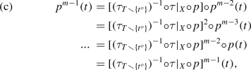
where the first equality holds by (b) at $n{=}m{-}1$, the second by (b) at $n{=}m{-}2$, ..., and the last by (b) at $n{=}1$. Finally, the claim holds because

$$\begin{aligned}\begin{gathered} t^o = p^m(t) = p{ \circ }p^{m-1}(t) = p{ \circ }[({ \tau }|_{T{ \smallsetminus }{ \lbrace }t^o{ \rbrace }})^{-1}{ \circ }{ \tau }|_X{ \circ }p]^{m-1}(t), \nonumber \end{gathered}\end{aligned}$$

where the first equality holds by the definition of m, the second is a rearrangement, and the third holds by (c).

Claim 8 : :

[T2$\,{}^{\prime }$] holds. Take $t{}^{\prime }{ \ }{ \in }{ \ }T{}^{\prime }{ \smallsetminus }{ \lbrace }t^{\prime o}{ \rbrace }$. Then Claim 1 implies $({ \tau }|_{T{ \smallsetminus }{ \lbrace }t^o{ \rbrace }})^{-1}(t{}^{\prime })$ ${ \in }$ $T{ \smallsetminus }{ \lbrace }t^o{ \rbrace }$. Thus by Claim 7, there exists $m{ \ }{ \ge }{ \ }1$ such that

$$\begin{aligned}\begin{gathered} t^o = p{ \circ }[({ \tau }|_{T{ \smallsetminus }{ \lbrace }t^o{ \rbrace }})^{-1}{ \circ }{ \tau }|_X{ \circ }p]^{m-1}{ \circ }({ \tau }|_{T{ \smallsetminus }{ \lbrace }t^o{ \rbrace }})^{-1}(t{}^{\prime }). \nonumber \end{gathered}\end{aligned}$$

It can now be argued that

$$\begin{aligned} t^{\prime o}=&{ \ }{ \tau }|_X(t^o) \nonumber \\ =&{ \ }{ \tau }|_X{ \circ }p{ \circ }[({ \tau }|_{T{ \smallsetminus }{ \lbrace }t^o{ \rbrace }})^{-1}{ \circ }{ \tau }|_X{ \circ }p]^{m-1}{ \circ }({ \tau }|_{T{ \smallsetminus }{ \lbrace }t^o{ \rbrace }})^{-1}(t{}^{\prime }) \nonumber \\ =&{ \ }[{ \tau }|_X{ \circ }p{ \circ }({ \tau }^{-1}|_{T{ \smallsetminus }{ \lbrace }t^o{ \rbrace }})^{-1}]^m(t{}^{\prime }) \nonumber \\ =&{ \ }(p{}^{\prime })^m(t{}^{\prime }). \nonumber \end{aligned}$$

The first equation holds by the definition of $t^{\prime o}$ and the fact that $t^o{ \ }{ \in }{ \ }X$ in any functioned tree (by remark [iv] in the paragraph following SP Eq. (1)). The second equation holds by the definition of m, the third is a rearrangement, and the fourth holds by Claim 5.

  $\square$

Fig. 8

$\mathbf {Set}$ diagram for Claims 3 and 5

Lemma A.14

Suppose ${ \varPi }= (T,C,{ \otimes })$ is an $\mathbf {NCP}$ preform. Also suppose ${ \tau }{:}T\rightarrow T{}^{\prime }$ and ${ \delta }{:}C\rightarrow C{}^{\prime }$ are bijections. Define ${ \otimes }{}^{\prime }$ by surjectivity and ${ \otimes }{}^{\prime \,\mathsf {gr}}=$${ \lbrace }\,({ \tau }(t),{ \delta }(c),{ \tau }(t^{\sharp })\,|\,$ $(t,c,t^{\sharp }){ \in }{ \otimes }^{\mathsf {gr}}\,{ \rbrace }$. Also define ${ \varPi }{}^{\prime } = (T{}^{\prime },C{}^{\prime },{ \otimes }{}^{\prime })$. Then (a) ${ \varPi }{}^{\prime }$ is an $\mathbf {NCP}$ preform and (b) $[{ \varPi },{ \varPi }{}^{\prime },{ \tau },{ \delta }]$ is an $\mathbf {NCP}$ isomorphism.

Proof

(a). By [P1] there exist $F{:}T{ \rightrightarrows } C$ and $t^o{ \ }{ \in }{ \ }T$ such that ${ \otimes }$ is a bijection from $F^{\mathsf {gr}}$ onto $T{ \smallsetminus }{ \lbrace }t^o{ \rbrace }$. Define $F{}^{\prime }{:}T{}^{\prime }{ \rightrightarrows } C{}^{\prime }$ by $F{}^{\prime \,\mathsf {gr}}=$ ${ \lbrace }({ \tau }(t),{ \delta }(c))|(t,c){ \in }F^{\mathsf {gr}}{ \rbrace }$. Also define $t^{\prime o}= { \tau }(t^o)$. It suffices to show that

This is done by Claims 6, 7, and 9.

 

Claim 1::

$({ \tau },{ \delta })|_{F^{\mathsf {gr}}}{:}F^{\mathsf {gr}}\rightarrow F{}^{\prime \,\mathsf {gr}}$ is a bijection. This follows from the bijectivity of ${ \tau }$, the bijectivity of ${ \delta }$, and the definition of $F{}^{\prime }$.

Claim 2::

${ \tau }|_{{ \tau }{ \smallsetminus }{ \lbrace }t^o{ \rbrace }}{:}T{ \smallsetminus }{ \lbrace }t^o{ \rbrace }\rightarrow T{}^{\prime }{ \smallsetminus }{ \lbrace }t^{\prime o}{ \rbrace }$ is a bijection. This follows from the bijectivity of ${ \tau }$ and the definition of $t^{\prime o}$.

Claim 3::

${ \tau }|_{{ \tau }{ \smallsetminus }{ \lbrace }t^o{ \rbrace }}{ \circ }{ \otimes }{ \circ }[({ \tau },{ \delta })|_{F^{\mathsf {gr}}}]^{-1}$ is a bijection from $F{}^{\prime \,\mathsf {gr}}$ onto $T{}^{\prime }{ \smallsetminus }{ \lbrace }t^{\prime o}{ \rbrace }$. The claim follows from composition. In particular, $(({ \tau },{ \delta })|_{F^{\mathsf {gr}}})^{-1}{:}F{}^{\prime \,\mathsf {gr}}\rightarrow F^{\mathsf {gr}}$ is a bijection by Claim 1, ${ \otimes }{:}F^{\mathsf {gr}}\rightarrow T{ \smallsetminus }{ \lbrace }t^o{ \rbrace }$ is a bijection by the definitions of F and $t^o$, and ${ \tau }_{T{ \smallsetminus }{ \lbrace }t^o{ \rbrace }}{:}T{ \smallsetminus }{ \lbrace }t^o{ \rbrace }\rightarrow T{}^{\prime }{ \smallsetminus }{ \lbrace }t^{\prime o}{ \rbrace }$ is a bijection by Claim 2. These three functions appear on the top, left, and bottom of Fig. 9.

Claim 4::

${ \otimes }{}^{\prime \,\mathsf {gr}}= ({ \tau }|_{T{ \smallsetminus }{ \lbrace }t^o{ \rbrace }}{ \circ }{ \otimes }{ \circ }[({ \tau },{ \delta })|_{F^{\mathsf {gr}}}]^{-1})^{\mathsf {gr}}$. It will be argued that

$$\begin{aligned} { \otimes }{}^{\prime \,\mathsf {gr}}&={ \ }{ \lbrace }\,({ \tau }(t),{ \delta }(c),{ \tau }(t^{\sharp }))\,|\,(t,c,t^{\sharp }){ \in }{ \otimes }^{\mathsf {gr}}\,{ \rbrace }\nonumber \\&={ \ }{ \lbrace }\,({ \tau }(t),{ \delta }(c),{ \tau }(t^{\sharp }))\,|\,(t,c){ \in }F^{\mathsf {gr}},\,t^{\sharp }{=}{ \otimes }(t,c)\,{ \rbrace }\nonumber \\&={ \ }{ \lbrace }\,(({ \tau },{ \delta })(t,c),{ \tau }|_{T{ \smallsetminus }{ \lbrace }t^o{ \rbrace }}{ \circ }{ \otimes }(t,c))\,|\,(t,c){ \in }F^{\mathsf {gr}}\,{ \rbrace }\nonumber \\&={ \ }{ \lbrace }\,(({ \tau },{ \delta })(t,c),{ \tau }|_{T{ \smallsetminus }{ \lbrace }t^o{ \rbrace }}{ \circ }{ \otimes }(t,c))\,|\,(t{}^{\prime },c{}^{\prime }){ \in }F{}^{\prime \,\mathsf {gr}},\,(t,c){=}[({ \tau },{ \delta })|_{F^{\mathsf {gr}}}]^{-1}(t{}^{\prime },c{}^{\prime })\,{ \rbrace }\nonumber \\&={ \ }{ \lbrace }\,(({ \tau },{ \delta }){ \circ }[({ \tau },{ \delta })|_{F^{\mathsf {gr}}}]^{-1}(t{}^{\prime },c{}^{\prime }),{ \tau }|_{T{ \smallsetminus }{ \lbrace }t^o{ \rbrace }}{ \circ }{ \otimes }{ \circ }[({ \tau },{ \delta })|_{F^{\mathsf {gr}}}]^{-1}(t{}^{\prime },c{}^{\prime })\,|\,(t{}^{\prime },c{}^{\prime }){ \in }F{}^{\prime \,\mathsf {gr}}\,{ \rbrace }\nonumber \\&={ \ }{ \lbrace }\,((t{}^{\prime },c{}^{\prime }), { \tau }|_{T{ \smallsetminus }{ \lbrace }t^o{ \rbrace }}{ \circ }{ \otimes }{ \circ }[({ \tau },{ \delta })|_{F^{\mathsf {gr}}}]^{-1} (t{}^{\prime },c{}^{\prime })\,|\,(t{}^{\prime },c{}^{\prime }){ \in }F{}^{\prime \,\mathsf {gr}}\,{ \rbrace }\nonumber \\&={ \ }(\,{ \tau }|_{T{ \smallsetminus }{ \lbrace }t^o{ \rbrace }}{ \circ }{ \otimes }{ \circ }[({ \tau },{ \delta })|_{F^{\mathsf {gr}}}]^{-1}\,)^{\mathsf {gr}}. \nonumber \end{aligned}$$

The first equality holds by the lemma’s definition of ${ \otimes }{}^{\prime }$. The second holds by the definition of F, and the third by the definition of $t^o$. The fourth holds by Claim 1. The fifth and sixth are rearrangements. The seventh holds by Claim 1.

Claim 5::

${ \otimes }{}^{\prime } = { \tau }|_{T{ \smallsetminus }{ \lbrace }t^o{ \rbrace }}{ \circ }{ \otimes }{ \circ }[({ \tau },{ \delta })|_{F^{\mathsf {gr}}}]^{-1}$, that is, Fig. 9 commutes. This follows from Claim 4 because [a] ${ \otimes }{}^{\prime }$ is surjective by definition and [b] ${ \tau }|_{T{ \smallsetminus }{ \lbrace }t^o{ \rbrace }}$ is surjective by Claim 2.

Claim 6::

[P1 ${}^{\prime }$] holds. This follows from Claims 3 and 5.

Claim 7::

[P2 ${}^{\prime }$] holds. Define p by [P2]. [P2] implies that [a] (T, p) is a functioned tree. Define $p{}^{\prime }$ by [P2${}^{\prime }$]. Claim 6 and SP Lemma C.1(a) implies [b] $p{}^{\prime }$ is well-defined and [c] $p{}^{\prime }$ is surjective. Because of [b], it suffices to show that $(T{}^{\prime },p{}^{\prime })$ is a functioned tree.

Toward that end, consider Lemma A.13. Lemma A.13’s assumptions are met by [a] and the bijectivity of ${ \tau }$. Thus Lemma A.13 implies that $(T{}^{\prime },p^{\star })$ is a functioned tree, where the function $p^{\star }$ is defined by [d] $p^{\star }$ being surjective and [e] ${{p^{\star }}{^{\mathsf {gr}}}} = { \lbrace }\,({ \tau }(t^{\sharp }),{ \tau }(t))\,|\,(t^{\sharp },t){ \in }p^{\mathsf {gr}}\,{ \rbrace }$. Thus it suffices to show that $p{}^{\prime } = p^{\star }$.

Toward that end, note [c] and [d] imply that both $p{}^{\prime }$ and $p^{\star }$ are surjective. Thus it suffices to show $p{}^{\prime \,\mathsf {gr}}= {{p^{\star }}{^{\mathsf {gr}}}}$. It will be argued that

$$\begin{aligned} p{}^{\prime \,\mathsf {gr}}=&{ \ }{ \lbrace }{ \ }(t^{\prime \sharp },t{}^{\prime }){ \in }(T{}^{\prime })^2{ \ }|{ \ }({ \exists } c{}^{\prime }{ \in }C{}^{\prime })(t{}^{\prime },c{}^{\prime },t^{\prime \sharp }){ \in }{ \otimes }{}^{\prime \,\mathsf {gr}}{ \ }{ \rbrace }\nonumber \\ =&{ \ }{ \lbrace }{ \ }(t^{\prime \sharp },t{}^{\prime }){ \in }(T{}^{\prime })^2{ \ }|{ \ }({ \exists } c{}^{\prime }{ \in }C{}^{\prime })({ \exists } (t,c,t^{\sharp }){ \in }{ \otimes }^{\mathsf {gr}}){ \ }(t{}^{\prime },c{}^{\prime },t^{\prime \sharp }){=}({ \tau }(t),{ \delta }(c),{ \tau }(t^{\sharp })){ \ }{ \rbrace }\nonumber \\ =&{ \ }{ \lbrace }{ \ }(t^{\prime \sharp },t{}^{\prime }){ \in }(T{}^{\prime })^2{ \ }|{ \ }({ \exists } (t,c,t^{\sharp }){ \in }{ \otimes }^{\mathsf {gr}}){ \ }(t{}^{\prime },t^{\prime \sharp }){=}({ \tau }(t),{ \tau }(t^{\sharp })){ \ }{ \rbrace }\nonumber \\ =&{ \ }{ \lbrace }{ \ }({ \tau }(t^{\sharp }),{ \tau }(t)){ \ }|{ \ }({ \exists } c{ \in }C)(t,c,t^{\sharp }){ \in }{ \otimes }^{\mathsf {gr}}{ \ }{ \rbrace }\nonumber \\ =&{ \ }{ \lbrace }{ \ }({ \tau }(t^{\sharp }),{ \tau }(t)){ \ }|{ \ }(t^{\sharp },t){ \in }p^{\mathsf {gr}}{ \ }{ \rbrace }\nonumber \\ =&{ \ }{{p^{\star }}{^{\mathsf {gr}}}}. \nonumber \end{aligned}$$

The first equality holds by the definition of $p{}^{\prime }$ two paragraphs ago, and the second equality holds by the definition of ${ \otimes }{}^{\prime }$ in the lemma statement. The ${ \subseteq }$ direction of the third equality holds simply because the variable $c{}^{\prime }$ does not appear in the right-hand side. The ${ \supseteq }$ direction follows from ${ \otimes }^{\mathsf {gr}}{ \ }{ \subseteq }{ \ }T{ \times }C{ \times }T$ and ${ \delta }{:}C\rightarrow C{}^{\prime }$. The fourth equality holds because the codomain of ${ \tau }$ is $T{}^{\prime }$. The fifth equality follows from the definition of p two paragraphs ago, and the sixth equality follows from [e].

Claim 8::

$({ \forall }c{}^{\prime }{ \in }C{}^{\prime }){ \ }(F{}^{\prime })^{-1}(c{}^{\prime }) = { \tau }(F^{-1}({ \delta }^{-1}(c{}^{\prime })))$. Take $c{}^{\prime }{ \ }{ \in }{ \ }C{}^{\prime }$. It is argued, in seven steps, that $(F{}^{\prime })^{-1}(c{}^{\prime })$ by definition is ${ \lbrace }t{}^{\prime }{ \in }T{}^{\prime }|c{}^{\prime }{ \in }F{}^{\prime }(t{}^{\prime }){ \rbrace }$, which by rearrangement is ${ \lbrace }t{}^{\prime }{ \in }T{}^{\prime }|(t{}^{\prime },c{}^{\prime }){ \in }F{}^{\prime \,\mathsf {gr}}{ \rbrace }$, which, by the definition of $F{}^{\prime }$, the bijectivity of ${ \tau }$, and the bijectivity of ${ \delta }$, is ${ \lbrace }t{}^{\prime }{ \in }T{}^{\prime }|({ \tau }^{-1}(t{}^{\prime }),{ \delta }^{-1}(c{}^{\prime })){ \in }F^{\mathsf {gr}}{ \rbrace }$, which by the bijectivity of ${ \tau }$ is ${ \lbrace }t{}^{\prime }|({ \exists } t{ \in }T)\,t{}^{\prime }{=}{ \tau }(t),\,({ \tau }^{-1}(t{}^{\prime }),{ \delta }^{-1}(c{}^{\prime })){ \in }F^{\mathsf {gr}}{ \rbrace }$, which by rearrangement is ${ \lbrace }{ \tau }(t)|({ \exists } t{ \in }T)({ \tau }^{-1}{ \circ } { \tau }(t),{ \delta }^{-1}(c{}^{\prime })){ \in }F^{\mathsf {gr}}{ \rbrace }$, which by rearrangement is ${ \tau }({ \lbrace }t{ \in }T|(t,{ \delta }^{-1}(c{}^{\prime })){ \in } F^{\mathsf {gr}}{ \rbrace }$, which by rearrangement is ${ \tau }(F^{-1}({ \delta }^{-1}(c{}^{\prime })))$.

Claim 9::

[P3 ${}^{\prime }$] holds. It must be shown that

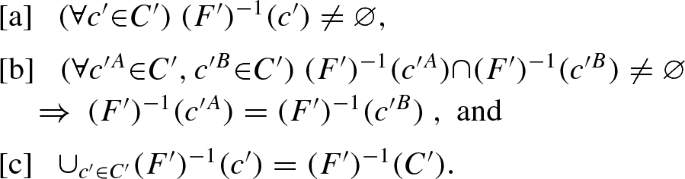
To show [a], take $c{}^{\prime }$. By the bijectivity of ${ \delta }$, ${ \delta }^{-1}(c{}^{\prime }){ \ }{ \in }{ \ }C$. Thus by [P3], $F^{-1}({ \delta }^{-1}(c{}^{\prime }))$ ${ \ne }$ ${ \varnothing }$. Thus ${ \tau }(F^{-1}({ \delta }^{-1}(c{}^{\prime }))){ \ }{ \ne }{ \ }{ \varnothing }$. Thus by Claim 8, $(F{}^{\prime })^{-1}(c{}^{\prime }){ \ }{ \ne }{ \ }{ \varnothing }$. To show [b], suppose that [b] were false. Then there would be $c{}^{\prime A}$ and $c{}^{\prime B}$ such that $(F{}^{\prime })^{-1}(c{}^{\prime A})$ and $(F{}^{\prime })^{-1}(c{}^{\prime B})$ intersect and are unequal. Hence by Claim 8, ${ \tau }(F^{-1}({ \delta }^{-1}(c{}^{\prime A})))$ and ${ \tau }(F^{-1}({ \delta }^{-1}(c{}^{\prime A})))$ intersect and are unequal. Hence by the bijectivity of ${ \tau }$, $F^{-1}({ \delta }^{-1}(c{}^{\prime A}))$ and $F^{-1}({ \delta }^{-1}(c{}^{\prime B}))$ intersect and are unequal. This contradicts [P3] because both ${ \delta }^{-1}(c{}^{\prime A})$ and ${ \delta }^{-1}(c{}^{\prime B})$ belong to C by the bijectivity of ${ \delta }$. Finally, [c] holds by definition (recall the last sentence of note 5).

 

Fig. 9

$\mathbf {Set}$ diagram for Claims 3 and 5

(b). This paragraph shows that $[{ \varPi },{ \varPi }{}^{\prime },{ \tau },{ \delta }]$ is a morphism. ${ \varPi }$ is a preform by assumption and ${ \varPi }{}^{\prime }$ is a preform by part (a). [PM1] and [PM2] hold by assumption (a fortiori). [PM3] holds with equality by the definition of ${ \otimes }{}^{\prime }$.

Finally, SP Theorem 3.7 implies that $[{ \varPi },{ \varPi }{}^{\prime },{ \tau },{ \delta }]$ is an isomorphism because [a] it is a morphism by the previous paragraph and [b] ${ \tau }$ and ${ \delta }$ are bijective by assumption. $\square$

Lemma A.15

Suppose ${ \varPhi }= (I,T,(C_i)_{i{ \in }I},{ \otimes })$ is an $\mathbf {NCF}$ form. Also suppose ${ \iota }{:}I\rightarrow I{}^{\prime }$, ${ \tau }{:}T\rightarrow T{}^{\prime }$, and ${ \delta }{:}{ \cup }_{i{ \in }I}C_i\rightarrow C{}^{\prime }$ are bijections. Define ${ \otimes }{}^{\prime }$ by surjectivity and ${ \otimes }{}^{\prime \,\mathsf {gr}}= { \lbrace }({ \tau }(t),{ \delta }(c),{ \tau }(t^{\sharp })|(t,c,t^{\sharp }){ \in }{ \otimes }^{\mathsf {gr}}{ \rbrace }$. Also define $(C{}^{\prime }_{i{}^{\prime }})_{i{}^{\prime }{ \in }I{}^{\prime }}$ at each $i{}^{\prime }$ by $C{}^{\prime }_{i{}^{\prime }} = { \delta }(C_{{ \iota }^{-1}(i{}^{\prime })})$. Also define ${ \varPhi }{}^{\prime } = (I{}^{\prime },T{}^{\prime },(C{}^{\prime }_{i{}^{\prime }})_{i{}^{\prime }{ \in }I{}^{\prime }},{ \otimes }{}^{\prime })$. Then (a) ${ \varPhi }{}^{\prime }$ is an $\mathbf {NCF}$ form and (b) $[{ \varPhi },{ \varPhi }{}^{\prime },{ \iota },{ \tau },{ \delta }]$ is an $\mathbf {NCF}$ isomorphism.

Proof

Define $C = { \cup }_{i{ \in }I}C_i$. Define ${ \varPi }= (T,C,{ \otimes })$. Define ${ \varPi }{}^{\prime } = (T{}^{\prime },C{}^{\prime },{ \otimes }{}^{\prime })$.  

Claim 1 : :

(a) ${ \varPi }{}^{\prime }$ is an $\mathbf {NCP}$ preform and (b) $[{ \varPi },{ \varPi }{}^{\prime },{ \tau },{ \delta }]$ is an $\mathbf {NCP}$ isomorphism. Consider Lemma A.14. The assumptions of Lemma A.14 are met because [i] ${ \varPi }$ is an $\mathbf {NCP}$ preform by [F1], [ii] ${ \tau }{:}T\rightarrow T{}^{\prime }$ is a bijection by assumption, and [iii] ${ \delta }{:}C\rightarrow C{}^{\prime }$ is a bijection because $C = { \cup }_{i{ \in }I}C_i$ by definition and ${ \delta }{:}{ \cup }_{i{ \in }I}C_i\rightarrow C{}^{\prime }$ is a bijection by assumption. Further, Lemma A.14’s definitions of ${ \otimes }{}^{\prime }$ and ${ \varPi }{}^{\prime }$ coincide with the present definitions of ${ \otimes }{}^{\prime }$ and ${ \varPi }{}^{\prime }$. Thus Lemma A.14 implies this claim’s two conclusions.

Claim 2 : :

$C{}^{\prime } = { \cup }_{i{}^{\prime }{ \in }I{}^{\prime }}C{}^{\prime }_{i{}^{\prime }}$. It is argued, in four steps, that $C{}^{\prime }$ by the bijectivity of ${ \delta }$ equals ${ \delta }({ \cup }_{i{ \in }I}C_i)$, which by rearrangement equals ${ \cup }_{i{ \in }I}{ \delta }(C_i)$, which by the bijectivity of ${ \iota }$ equals ${ \cup }_{i{}^{\prime }{ \in }I{}^{\prime }}{ \delta }(C_{{ \iota }^{-1}(i{}^{\prime })})$, which by the definition of $(C{}^{\prime }_{i{}^{\prime }})_{i{}^{\prime }{ \in }I{}^{\prime }}$ equals ${ \cup }_{i{}^{\prime }{ \in }I{}^{\prime }}C{}^{\prime }_{i{}^{\prime }}$.

Claim 3 : :

${ \varPhi }{}^{\prime }$ satisfies [F1]. It must be shown that $(T{}^{\prime },C^{\star },{ \otimes }{}^{\prime })$ is a preform where $C^{\star }$ is defined as ${ \cup }_{i{}^{\prime }{ \in }I{}^{\prime }}C{}^{\prime }_{i{}^{\prime }}$. Claim 2 implies that $C^{\star }= C{}^{\prime }$. Hence ${ \varPi }{}^{\prime } = (T{}^{\prime },C^{\star },{ \otimes }{}^{\prime })$. Hence Claim 1(a) implies that $(T{}^{\prime },C^{\star },{ \otimes }{}^{\prime })$ is a preform.

Claim 4 : :

${ \varPhi }{}^{\prime }$ satisfies [F2]. Take $i{}^{\prime }{ \ }{ \in }{ \ }I{}^{\prime }$ and $j{}^{\prime }{ \ }{ \in }{ \ }I{}^{\prime }{ \smallsetminus }{ \lbrace }i{}^{\prime }{ \rbrace }$. The bijectivity of ${ \iota }$ implies ${ \iota }^{-1}(i{}^{\prime }){ \ }{ \in }{ \ }I$ and ${ \iota }^{-1}(j{}^{\prime }){ \ }{ \in }{ \ }I{ \smallsetminus }{ \lbrace }{ \iota }^{-1}(i{}^{\prime }){ \rbrace }$. Thus [F2] for ${ \varPhi }$ implies $C_{{ \iota }^{-1}(i{}^{\prime })}\,{ \cap }\,C_{{ \iota }^{-1}(j{}^{\prime })} = { \varnothing }$. Hence the bijectivity of ${ \delta }$ implies ${ \delta }(C_{{ \iota }^{-1}(i{}^{\prime })})\,{ \cap } { \delta }(C_{{ \iota }^{-1}(j{}^{\prime })}) = { \varnothing }$. Hence the definition of $(C{}^{\prime }_{i{}^{\prime }})_{i{}^{\prime }{ \in }I{}^{\prime }}$ implies $C{}^{\prime }_{i{}^{\prime }}{ \cap }C{}^{\prime }_{j{}^{\prime }} = { \varnothing }$.

Claim 5 : :

${ \varPhi }{}^{\prime }$ satisfies [F3]. Take $t{}^{\prime }{ \ }{ \in }{ \ }T{}^{\prime }$. The bijectivity of ${ \tau }$ implies ${ \tau }^{-1}(t{}^{\prime }){ \ }{ \in }{ \ }T$. Hence [F3] for ${ \varPhi }$ implies there is $i{ \ }{ \in }{ \ }I$ such that $F({ \tau }^{-1}(t{}^{\prime })){ \ }{ \subseteq }{ \ }C_i$. Hence the bijectivity of ${ \iota }$ implies there is $i{}^{\prime }{ \ }{ \in }{ \ }I{}^{\prime }$ such that [a] $F({ \tau }^{-1}(t{}^{\prime })){ \ }{ \subseteq }{ \ }C_{{ \iota }^{-1}(i{}^{\prime })}$. Also, it will be shown [b] $F({ \tau }^{-1}(t{}^{\prime })) = { \delta }^{-1}(F{}^{\prime }(t{}^{\prime }))$ by arguing, in steps, that $F({ \tau }^{-1}(t{}^{\prime }))$ by rearrangement equals ${ \lbrace }c{ \in }C|({ \tau }^{-1}(t{}^{\prime }),c){ \in }F^{\mathsf {gr}}{ \rbrace }$, which by Claim 1(b) and SP Proposition 3.8(c) equals ${ \lbrace }c{ \in }C|(t{}^{\prime },{ \delta }(c)){ \in }F{}^{\prime \,\mathsf {gr}}{ \rbrace }$, which by the bijectivity of ${ \delta }$ equals ${ \lbrace }c|({ \exists } c{}^{\prime }{ \in }C{}^{\prime })$ $c{=}{ \delta }^{-1}(c{}^{\prime }),\,(t{}^{\prime },{ \delta }(c)){ \in }F{}^{\prime \,\mathsf {gr}}{ \rbrace }$, which by rearrangement equals ${ \lbrace }{ \delta }^{-1}(c{}^{\prime })|$ $({ \exists } c{}^{\prime }{ \in }C{}^{\prime })(t{}^{\prime },c{}^{\prime }){ \in }F{}^{\prime \,\mathsf {gr}}{ \rbrace }$, which by rearrangement equals ${ \delta }^{-1}({ \lbrace }c{}^{\prime }{ \in }C{}^{\prime }|(t{}^{\prime },c{}^{\prime }){ \in }F{}^{\prime \,\mathsf {gr}}{ \rbrace })$, which by rearrangement equals ${ \delta }^{-1}(F{}^{\prime }(t{}^{\prime }))$. [a] and [b] imply ${ \delta }^{-1}(F{}^{\prime }(t{}^{\prime })){ \ }{ \subseteq }{ \ }C_{{ \iota }^{-1}(i{}^{\prime })}$. Hence the bijectivity of ${ \delta }$ implies $F{}^{\prime }(t{}^{\prime }){ \ }{ \subseteq }{ \ }{ \delta }(C_{{ \iota }^{-1}(i{}^{\prime })})$. Hence the definition of $C{}^{\prime }_{i{}^{\prime }}$ implies $F{}^{\prime }(t{}^{\prime }){ \ }{ \subseteq }{ \ }C{}^{\prime }_{i{}^{\prime }}$.

Claim 6 : :

${ \varPhi }{}^{\prime }$ is an $\mathbf {NCF}$ form. This follows from Claims 3–5.

Claim 7 : :

$[{ \varPhi },{ \varPhi }{}^{\prime },{ \iota },{ \tau },{ \delta }]$ is an $\mathbf {NCF}$ morphism. ${ \varPhi }$ is an $\mathbf {NCF}$ form by assumption, and ${ \varPhi }{}^{\prime }$ is an $\mathbf {NCF}$ form by Claim 6. [FM1] holds because $[{ \varPi },{ \varPi }{}^{\prime },{ \tau },{ \delta }]$ is an $\mathbf {NCP}$ morphism a fortiori by Claim 1(b). [FM2] holds by assumption. For [FM3], take $i{ \ }{ \in }{ \ }I$. It is argued, in two steps, that ${ \delta }(C_i)$ by the bijectivity of ${ \iota }$ equals ${ \delta }(C_{{ \iota }^{-1}{ \circ }{ \iota }(i)})$, which by definition of $C{}^{\prime }_{{ \iota }(i)}$ equals $C{}^{\prime }_{{ \iota }(i)}$.

Claim 8 : :

$[{ \varPhi },{ \varPhi }{}^{\prime },{ \iota },{ \tau },{ \delta }]$ is an $\mathbf {NCF}$ isomorphism. This follows from the reverse direction of Corollary 2.5 because [a] $[{ \varPhi },{ \varPhi }{}^{\prime },{ \iota },{ \tau },{ \delta }]$ is an $\mathbf {NCF}$ morphism by Claim 7, [b] $[{ \varPi },{ \varPi }{}^{\prime },{ \tau },{ \delta }]$ is an $\mathbf {NCP}$ isomorphism by Claim 1(b), and [c] ${ \iota }$ is a bijection by assumption.

 

Conclusion. The lemma’s conclusions follow from Claims 6 and 8. $\square$

Appendix B: $\mathbf {CsqF}$

Proof B.1

(for Proposition 3.1). The proposition follows from Claims 1–8 and 13–14.  

Claim 1 : :

(a) holds. Suppose [a] $t^o{ \ }{ \ne }{ \ }{ \lbrace }{ \rbrace }$. [Csq1] states [b] ${ \lbrace }{ \rbrace }{ \ }{ \in }{ \ }T$. [a] and [b] imply ${ \lbrace }{ \rbrace }{ \ }{ \in }{ \ }T{ \smallsetminus }{ \lbrace }t^o{ \rbrace }$. Thus by [P1], there are $t{ \ }{ \in }{ \ }T$ and $c{ \ }{ \in }{ \ }C$ such that $(t,c,{ \lbrace }{ \rbrace }){ \ }{ \in }{ \ }{ \otimes }^{\mathsf {gr}}$. Thus by [Csq2], $p({ \lbrace }{ \rbrace }){ \oplus }(c)$ $= { \lbrace }{ \rbrace }$. This is impossible because the left-hand sequence has positive length and the right-hand sequence has zero length.

Claim 2 : :

(b) holds. Take $t^{\sharp }{ \ }{ \in }{ \ }T{ \smallsetminus }{ \lbrace }{ \lbrace }{ \rbrace }{ \rbrace }$. Claim 1 (a) implies $t^{\sharp }{ \ }{ \in }{ \ }T{ \smallsetminus }{ \lbrace }t^o{ \rbrace }$. Thus the reverse direction of SP Proposition 3.1(a) implies $(p(t^{\sharp }),q(t^{\sharp }),t^{\sharp })$ ${ \in }$ ${ \otimes }$. Thus [Csq2] implies $p(t^{\sharp }){ \oplus }(q(t^{\sharp })) = t^{\sharp }$. Thus $p(t^{\sharp }) = {_1t^{\sharp }_{|t^{\sharp }|-1}}$ and $q(t^{\sharp }) = t^{\sharp }_{|t^{\sharp }|}$.

Claim 3 : :

(c) holds. Assume $(t,c,t^{\sharp }){ \ }{ \in }{ \ }{ \otimes }^{\mathsf {gr}}$. Then [P1] yields $(t,c,t^{\sharp }){ \ }{ \in } { \ }T{ \times }C{ \times }T$, and [Csq2] yields $t{ \oplus }(c) = t^{\sharp }$. Conversely, suppose [1] $(t,c,t^{\sharp }){ \ }{ \in }{ \ }T{ \times }C{ \times }T$ and [2] $t{ \oplus }(c) = t^{\sharp }$. [2] implies [3] $t = {_1t^{\sharp }_{|t^{\sharp }|-1}}$ and [4] $c = t^{\sharp }_{|t^{\sharp }|}$. Further, [4] implies $t^{\sharp }{ \ }{ \ne }{ \ }{ \lbrace }{ \rbrace }$. This and [1] implies [5] $t^{\sharp }{ \ }{ \in }{ \ }T{ \smallsetminus }{ \lbrace }{ \lbrace }{ \rbrace }{ \rbrace }$. [5] and Claim 2 (b) imply [6] $p(t^{\sharp }) = {_1t^{\sharp }_{|t^{\sharp }|-1}}$ and [7] $q(t^{\sharp }) = t^{\sharp }_{|t^{\sharp }|}$. [3] and [6] imply [8] $t = p(t^{\sharp })$. [4] and [7] imply [9] $c = q(t^{\sharp })$. Further, [5] and Claim 1 (a) imply $t^{\sharp }{ \ }{ \ne }{ \ }t^o$, and thus SP Proposition 3.1(a) implies [10] $(p(t^{\sharp }),q(t^{\sharp }),t^{\sharp }){ \ }{ \in }{ \ }{ \otimes }^{\mathsf {gr}}$. [8]–[10] imply $(t,c,t^{\sharp }){ \ }{ \in }{ \ }{ \otimes }^{\mathsf {gr}}$.

Claim 4 : :

(d) holds. By [P1], $F^{\mathsf {gr}}{ \subseteq }{ \ }T{ \times }C$. Thus it suffices to show $({ \forall }t{ \in }T,c{ \in }C)$ $(t,c){ \ }{ \in }{ \ }F^{\mathsf {gr}}$ iff $t{ \oplus }c{ \ }{ \in }{ \ }T$. Suppose $(t,c){ \ }{ \in }{ \ }F^{\mathsf {gr}}$. Then [P1] implies there is [1] $t^{\sharp }{ \ }{ \in }{ \ }T$ such that [2] $(t,c,t^{\sharp }){ \ }{ \in }{ \ }{ \otimes }^{\mathsf {gr}}$. [2] and Claim 3 (c) imply $t{ \oplus }(c) = t^{\sharp }$. This and [1] imply $t{ \oplus }(c){ \ }{ \in }{ \ }T$. Conversely, suppose $t{ \oplus }(c){ \ }{ \in }{ \ }T$. There there is $t^{\sharp }{ \ }{ \in }{ \ }T$ such that $t{ \oplus }(c) = t^{\sharp }$. Thus Claim 3 (c) implies $(t,c,t^{\sharp }){ \ }{ \in }{ \ }{ \otimes }^{\mathsf {gr}}$. This and [P1] imply $(t,c){ \ }{ \in }{ \ }F^{\mathsf {gr}}$.

Claim 5 : :

(e) holds. Take $t{ \ }{ \in }{ \ }T$. The following induction is on $m{ \ }{ \in }{ \ }{ \lbrace }0,1,...\,|t|{ \rbrace }$. For the initial step, assume $m = 0$. Then $p^0(t) = t = {_1t_{|t|}} = {_1t_{|t|-0}} = {_1t_{|t|-m}}$ by inspection. For the inductive step, assume $m > 0$. Note $m{ \ }{ \le }{ \ }|t|$ implies $|t|{-}m{ \ }{ \ge }{ \ }0$, which implies $|t|{-}(m{-}1) > 0$, which implies [1] $_1t_{|t|-(m-1)}{ \ }{ \ne }{ \ }{ \lbrace }{ \rbrace }$. Then it is argued, in steps, that $p^m(t)$ by $m > 0$ equals $p(p^{m-1}(t))$, which by the inductive hypothesis equals $p(_1t_{|t|-(m-1)})$, which by [1] and Claim 2 (b) at $t^{\sharp }= {_1t_{|t|-(m-1)}}$ equals $_1t_{|t|-(m-1)-1}$, which by rearrangement equals $_1t_{|t|-m}$.

Claim 6 : :

(f) holds. Take $t{ \ }{ \in }{ \ }T$. It will be shown that $p^{|t|}(t) = t^0$ by arguing, in steps, that $p^{|t|}(t)$ by Claim 5 (e) at $m = |t|$ equals $_1t_{|t|-|t|}$, which equals $_1t_0$, which equals ${ \lbrace }{ \rbrace }$, which by Claim 1 (a) equals $t^o$. This and the definition of k imply $k(t) = |t|$.

Claim 7 : :

(g) holds. Take $t{ \ }{ \in }{ \ }T$. By inspection, the result is equivalent to $({ \forall }{ \ell }{ \in }{ \lbrace }1,2,...\,|t|{ \rbrace })$ $t_{ \ell }= q{ \circ }p^{|t|-{ \ell }}(t)$. On the one hand, take $t = { \lbrace }{ \rbrace }$. Then $|t| = 0$ so the result is vacuously true. On the other hand, take $t{ \ }{ \ne }{ \ }{ \lbrace }{ \rbrace }$. Then take [1] ${ \ell }{ \ }{ \in }{ \ }{ \lbrace }1,2,...\,|t|{ \rbrace }$. First it will be shown that [2] $p^{|t|-{ \ell }}(t) = {_1t_{ \ell }}$ by arguing, in steps, that $p^{|t|-{ \ell }}(t)$ by Claim 5 (e) at $m = |t|{-}{ \ell }$ equals $_1t_{|t|-(|t|-{ \ell })}$, which by rearrangement equals $_1t_{ \ell }$. Then it is argued, in steps, that $q{ \circ }p^{|t|-{ \ell }}(t)$ by [2] equals $q(_1t_{ \ell })$, which by [1] and Claim 2 (b) equals $t_{ \ell }$.

Claim 8 : :

(h) holds. Suppose $c{ \ }{ \in }{ \ }C$. This and [P3] imply $F^{-1}(c){ \ }{ \ne }{ \ }{ \varnothing }$. Thus there is $t^\star { \ }{ \in }{ \ }T$ such that $(t^\star ,c){ \ }{ \in }{ \ }F^{\mathsf {gr}}$. This and Claim 4 (d) imply $t^*{ \oplus }(c){ \ }{ \in }{ \ }T$. Thus $c{ \ }{ \in }{ \ }R(t^*{ \oplus }(c)){ \ }{ \subseteq }{ \ }{ \cup }{ \lbrace }R(t)|t{ \in }T{ \rbrace }$. Conversely, suppose $b{ \ }{ \in }{ \ }{ \cup }{ \lbrace }R(t)|t{ \in }T{ \rbrace }$. There there is [1] $t^*{ \ }{ \in }{ \ }T$ such that [2] $b{ \ }{ \in }{ \ }R(t^*)$. [1] and Claim 7 (g) imply that $t^* = (q{ \circ }p^{|t^*|-{ \ell }}(t^*))^{|t^*|}_{{ \ell }=1}$. This and [2] imply there is ${ \ell }^*{ \ }{ \in }{ \ }{ \lbrace }1,2,...\,|t^*|{ \rbrace }$ such that $b = q{ \circ }p^{|t^*|-{ \ell }^*}(t^*)$. This implies $b{ \ }{ \in }{ \ }C$ since the codomain of q is C by the definition of q.

Claim 9 : :

$({ \forall }t^A{ \in }T,t^B{ \in }T)$ $(|t^A|\,{<}\,|t^B|{ \ }\text {and}{ \ }t^A\,{=}\,{_1t^B_{|t^A|}})$ iff $t^A{ \ }{ \subset }{ \ }t^B$. Take $t^A{ \ }{ \in }{ \ }T$ and $t^B{ \ }{ \in }{ \ }T$. First, suppose [1] $|t^A| < |t^B|$ and [2] $t^A = {_1t^B_{|t^A|}}$. [1] and the definition of $_1t^B_{|t^A|}$ imply [3] $_1t^B_{|t^A|}{ \ }{ \subset }{ \ }t^B$. [2] and [3] imply $t^A{ \ }{ \subset }{ \ }t^B$. Conversely, suppose [4] $t^A{ \ }{ \subset }{ \ }t^B$. [Csq1] implies [5] $t^A = { \lbrace }(1,t^A_1),(2,t^A_2),...\,(|t^A|,t^A_{|t^A|}){ \rbrace }$ and [6] $t^B = { \lbrace }(1,t^B_1),(2,t^B_2),...(|t^B|,t^B_{|t^B|}){ \rbrace }$. By inspection, [4]–[6] imply $|t^A| < |t^B|$ and $t^A = {_1t^B_{|t^A|}}$.

Claim 10 : :

$({ \forall }t^A{ \in }T,t^B{ \in }T)$ $(|t^A|\,{ \le }\,|t^B|{ \ }\text {and}{ \ }t^A\,{=}\,{_1t^B_{|t^A|}})$ iff $t^A{ \ }{ \subseteq }{ \ }t^B$.²⁶ In the proof of Claim 9, change < to ${ \le }$, and ${ \subset }$ to ${ \subseteq }$.

Claim 11 : :

$({ \forall }t^A{ \in }T,t^B{ \in }T){ \ }t^A{ \ }{ \prec }{ \ }t^B$ iff $t^A{ \ }{ \subset }{ \ }t^B$. Take $t^A{ \ }{ \in }{ \ }T$ and $t^B{ \ }{ \in }{ \ }T$. First, suppose $t^A{ \ }{ \prec }{ \ }t^B$. This and the definition of ${ \prec }$ imply there is [1] $m{ \ }{ \in }{ \ }{ \lbrace }1,2,...\,k(t^B){ \rbrace }$ such that [2] $t^A = p^m(t^B)$. [1] and Claim 6 (f) imply [3] $m{ \ }{ \in }{ \ }{ \lbrace }1,2,...\,|t^B|{ \rbrace }$. Finally, it is argued, in steps, that $t^A$ by [2] equals $p^m(t^B)$, which by [3] and Claim 5 (e) equals ${_1t^B_{|t^B|-m}}$, which by [3] is a strict subset of $_1t^B_{|t^B|}$, which by inspection equals $t^B$. Conversely, suppose $t^A{ \ }{ \subset }{ \ }t^B$. This and Claim 9 imply [1] $|t^A| < |t^B|$ and [2] $t^A = {_1t^B_{|t^A|}}$. For convenience, let [3] $m = |t^B|{-}|t^A|$. Note [1] and $|t^A|{ \ }{ \ge }{ \ }0$ imply [4] $m{ \ }{ \in }{ \ }{ \lbrace }1,2,...\,|t^B|{ \rbrace }$. It will now be shown that [5] $t^A = p^m(t^B)$ by arguing, in steps, that $t^A$ by [2] equals $_1t^B_{|t^A|}$, which by [3] equals $_1t^B_{|t^B|-m}$, which by [4] and Claim 5 (e) at $t = t^B$ equals $p^m(t^B)$. Finally, [5], [4], and the definition of ${ \prec }$ imply $t^A{ \ }{ \prec }{ \ }t^B$.

Claim 12 : :

$({ \forall }t^A{ \in }T,t^B{ \in }T){ \ }t^A{ \ }{ \preccurlyeq }{ \ }t^B$ iff $t^A{ \ }{ \subseteq }{ \ }t^B$. Take $t^A{ \ }{ \in }{ \ }T$ and $t^B{ \ }{ \in }{ \ }T$. First, suppose $t^A{ \ }{ \preccurlyeq }{ \ }t^B$. Then by the definition of ${ \preccurlyeq }$, either $t^A{ \ }{ \prec }{ \ }t^B$ or $t^A = t^B$. In the first case, Claim 11 implies $t^A{ \ }{ \subset }{ \ }t^B$. Thus $t^A{ \ }{ \subseteq }{ \ }t^B$ in both cases. Conversely, suppose $t^A{ \ }{ \subseteq }{ \ }t^B$. Then either $t^A{ \ }{ \subset }{ \ }t^B$ or $t^A = t^B$. In the first case, Claim 11 implies $t^A{ \ }{ \prec }{ \ }t^B$. Thus the definition of ${ \preccurlyeq }$ implies $t^A{ \ }{ \preccurlyeq }{ \ }t^B$ in both cases.

Claim 13 : :

(i) holds. Combine Claims 9 and 11.

Claim 14 : :

(j) holds. Combine Claims 10 and 12.

  $\square$

Lemma B.2

Suppose $(T,C,{ \otimes })$ is a node-and-choice preform with its $t^o$, p, q, and k. Let $\bar{T}= { \lbrace }\,(q{ \circ }p^{k(t)-{ \ell }}(t))^{k(t)}_{{ \ell }=1}\,|\,t{ \in }T\,{ \rbrace }$. Then

$$\begin{aligned}\begin{gathered} T{ \ }{ \ni }{ \ }t{ \ }\mapsto { \ }(q{ \circ }p^{k(t)-{ \ell }}(t))^{k(t)}_{{ \ell }=1}{ \ }{ \in }{ \ }\bar{T}\nonumber \end{gathered}\end{aligned}$$

is a well-defined bijection. Its inverse is

(to be clear, ).

Proof

Let ${ \alpha }$ be the function from T to $\bar{T}$, and conversely, let ${ \beta }$ be the function to T from $\bar{T}$.

This paragraph shows that ${ \beta }{ \circ }{ \alpha }$ is the identity function on T. The composition is well-defined because [1] the domain of ${ \beta }$ is $\bar{T}$ and [2] the range of ${ \alpha }$ is $\bar{T}$ by the definition of $\bar{T}$. Thus it suffices to show $({ \forall }t{ \in }T){ \ }{ \beta }{ \circ }{ \alpha }(t) = t$. Toward that end, take $t{ \ }{ \in }{ \ }T$. First, suppose $k(t) = 0$. It is argued, in steps, that ${ \beta }{ \circ }{ \alpha }(t)$ by the definition of ${ \alpha }$ equals ${ \beta }({ \lbrace }{ \rbrace })$, which by the definition of ${ \beta }$ equals $t^o$, which by $k(t) = 0$ equals t. Second, suppose $k(t) = 1$. It is argued, in steps, that ${ \beta }{ \circ }{ \alpha }(t)$ by the definition of ${ \alpha }$ equals ${ \beta }[(q(t))]$, which by the definition of ${ \beta }$ equals $t^o{ \otimes }q(t)$, which by $k(t) = 1$ equals $p(t){ \otimes }q(t)$, which by SP Proposition 3.1(b) equals t. Third and finally, suppose $k(t){ \ }{ \ge }{ \ }2$. It will be argued that

$$\begin{aligned} { \beta }{ \circ }{ \alpha }(t) =&{ \ }{ \beta }({ \ }(q{ \circ }p^{k(t)-{ \ell }}(t))^{k(t)}_{{ \ell }=1}{ \ }) \nonumber \\ =&{ \ }[[...[[t^o{ \otimes }q{ \circ }p^{k(t)-1}(t)]{ \otimes }q{ \circ }p^{k(t)-2}(t)]\,...{ \ }]{ \otimes }q{ \circ }p(t)]{ \otimes }q(t) \nonumber \\ =&{ \ }[[...[[p^{k(t)}(t){ \otimes }q{ \circ }p^{k(t)-1}(t)]{ \otimes }q{ \circ }p^{k(t)-2}(t)]\,...{ \ }]{ \otimes }q{ \circ }p(t)]{ \otimes }q(t) \nonumber \\ =&{ \ }[[...[[p{ \circ }p^{k(t)-1}(t){ \otimes }q{ \circ }p^{k(t)-1}(t)]{ \otimes }q{ \circ }p^{k(t)-2}(t)]\,...{ \ }]{ \otimes }q{ \circ }p(t)]{ \otimes }q(t) \nonumber \\ =&{ \ }[[...[p^{k(t)-1}(t){ \otimes }q{ \circ }p^{k(t)-2}]\,...{ \ }]{ \otimes }q{ \circ }p(t)]{ \otimes }q(t) \nonumber \\&{ \ }{ \cdot }{ \ }{ \cdot }{ \ }{ \cdot }\nonumber \\ =&{ \ }p(t){ \otimes }q(t) = t. \nonumber \end{aligned}$$

The first equality holds by the definition of ${ \alpha }$, the second by the definition of ${ \beta }$, and the third by the definition of k. The fourth and fifth equalities hold by a rearrangement and SP Proposition 3.1(b). The sixth equality holds by $k(t){-}2$ similar applications of SP Proposition 3.1(b), and the final equality holds by a final application of SP Proposition 3.1(b).

This paragraph shows that ${ \alpha }{ \circ }{ \beta }$ is the identity function on $\bar{T}$. The composition is well-defined because [a] the domain of ${ \alpha }$ is T and [b] each value of ${ \beta }$ is a value of ${ \otimes }$ and the codomain of ${ \otimes }$ is a subset of T. Thus it suffices to show $({ \forall }\bar{t}{ \in }\bar{T}){ \ }{ \alpha }{ \circ }{ \beta }(\bar{t}) = \bar{t}$. Toward that end, take $\bar{t}$. First, suppose $\bar{t}= { \lbrace }{ \rbrace }$. It will be argued, in steps, that ${ \alpha }{ \circ }{ \beta }({ \lbrace }{ \rbrace })$ by the definition of ${ \beta }$ equals ${ \alpha }(t^o)$, which by the definition of ${ \alpha }$ equals ${ \lbrace }{ \rbrace }$. Second, suppose $\bar{t}{ \ }{ \ne }{ \ }{ \lbrace }{ \rbrace }$. Then it suffices to show that $({ \forall }{ \ell }{ \in }{ \lbrace }1,2,...|\bar{t}|{ \rbrace })$ $({ \alpha }{ \circ }{ \beta }(\bar{t}))_{ \ell }= \bar{t}_{ \ell }$. Toward this end, take ${ \ell }$. [i] First assume ${ \ell }< |\bar{t}|$. It will be argued that

$$\begin{aligned} ({ \alpha }{ \circ }{ \beta }(\bar{t}))_{ \ell }=&{ \ }q{ \circ }p^{k({ \beta }(\bar{t}))-{ \ell }}({ \beta }(\bar{t})) \nonumber \\ =&{ \ }q{ \circ }p^{|\bar{t}|-{ \ell }}({ \beta }(\bar{t})) \nonumber \\ =&{ \ }q{ \circ }p^{|\bar{t}|-{ \ell }}[{ \ }((...((t^o{ \otimes }\bar{t}_1){ \otimes }\bar{t}_2)\,\dots \,){ \otimes }\bar{t}_{|\bar{t}|-1}){ \otimes }\bar{t}_{|\bar{t}|}{ \ }] \nonumber \\ =&{ \ }q{ \circ }p^{|\bar{t}|-{ \ell }-1}[{ \ }((...((t^o{ \otimes }\bar{t}_1){ \otimes }\bar{t}_2)\,\dots \,){ \otimes }\bar{t}_{|\bar{t}|-2}){ \otimes }\bar{t}_{|\bar{t}|-1}{ \ }] \nonumber \\&{ \ }{ \cdot }{ \ }{ \cdot }{ \ }{ \cdot }\nonumber \\ =&{ \ }q{ \circ }p^{|\bar{t}|-{ \ell }-(|\bar{t}|-{ \ell })}[{ \ }((...((t^o{ \otimes }\bar{t}_1){ \otimes }\bar{t}_2)\,\dots \,){ \otimes }\bar{t}_{|\bar{t}|-(|\bar{t}|-{ \ell })-1}){ \otimes }\bar{t}_{|\bar{t}|-(|\bar{t}|-{ \ell })}{ \ }] \nonumber \\ =&{ \ }q{ \circ }p^0[{ \ }((...((t^o{ \otimes }\bar{t}_1){ \otimes }\bar{t}_2)\,\dots \,){ \otimes }\bar{t}_{{ \ell }-1}){ \otimes }\bar{t}_{ \ell }{ \ }] = \bar{t}_{ \ell }. \nonumber \end{aligned}$$

The first equality holds by the definition of ${ \alpha }$. The second equality holds because $k({ \beta }(\bar{t})) = |\bar{t}|$ by inspecting the definitions of k and ${ \beta }$. The third holds by the definition of ${ \beta }$. The fourth holds by the definition of p. The fifth holds by $|t|{-}{ \ell }{-}1$ similar applications of the definition of p. The sixth is a rearrangement. The seventh holds by the definition of q. [ii] Second assume ${ \ell }= |\bar{t}|$. Then it will be argued that

$$\begin{aligned} \begin{array}{c} ({ \alpha }{ \circ }{ \beta }(\bar{t}))_{|\bar{t}|} = q{ \circ }p^{k({ \beta }(\bar{t}))-|\bar{t}|}({ \beta }(\bar{t})) \nonumber \\ = q{ \circ }p^{|\bar{t}|-|\bar{t}|}({ \beta }(\bar{t})) = q({ \beta }(\bar{t})) = \bar{t}_{|\bar{t}|}{ \ }, \nonumber \end{array} \end{aligned}$$

The first equality holds by the definition of ${ \alpha }$ and ${ \ell }= |\bar{t}|$. The second equality holds because $k({ \beta }(\bar{t})) = |\bar{t}|$ by inspecting the definitions of k and ${ \beta }$. The third is trivial. The fourth holds by the definitions of q and ${ \beta }$. $\square$

Proof B.3

(for Theorem 3.2).

(a). Lemma B.2 implies $\bar{{ \tau }}{:}T\rightarrow \bar{T}$ is a bijection. Thus the assumptions of Lemma A.14 are met at $T{}^{\prime } = \bar{T}$, $C{}^{\prime } = C$, and ${ \delta }= \mathsf {id}_C$. Further, the definition of $\bar{{ \otimes }}$ here coincides with the definition of ${ \otimes }{}^{\prime }$ in Lemma A.14. Therefore Lemma A.14 implies that $(\bar{T},C,\bar{{ \otimes }})$ is an $\mathbf {NCP}$ preform, and that $[(T,C,{ \otimes }),(\bar{T},C,\bar{{ \otimes }}),\bar{{ \tau }},\mathsf {id}_C]$ is an $\mathbf {NCP}$ isomorphism. Thus [Csq1] and [Csq2] remain to be shown.

For [Csq1], note that the definition of $\bar{T}$ implies that $\bar{T}$ is a collection of finite sequences. Further, since $t^o{ \ }{ \in }{ \ }T$ by [P1], the definition of $\bar{T}$ implies that $(q{ \circ }p^{k(t^o)-{ \ell }}(t^o))^{k(t^o)}_{{ \ell }=1}{ \ }{ \in }{ \ }\bar{T}$. Thus, since $k(t^o) = 0$ by the definition of k, $(q{ \circ }p^{0-{ \ell }}(t^o))^0_{{ \ell }=1}{ \ }{ \in }{ \ }\bar{T}$. Thus ${ \lbrace }{ \rbrace }{ \ }{ \in }{ \ }\bar{T}$.

For [Csq2], take $(\bar{t},c,\bar{t}^{\sharp }){ \ }{ \in }{ \ }\bar{{ \otimes }}$. Then by the definition of $\bar{{ \otimes }}$, there are $t{ \ }{ \in }{ \ }T$ and $t^{\sharp }{ \ }{ \in }{ \ }T$ such that [a] $\bar{{ \tau }}(t) = \bar{t}$, [b] $\bar{{ \tau }}(t^{\sharp }) = \bar{t}^{\sharp }$, and [c] $(t,c,t^{\sharp }){ \ }{ \in }{ \ }{ \otimes }^{\mathsf {gr}}$. [a], [b], and the definition of $\bar{{ \tau }}$ imply [d] $\bar{t}= (q{ \circ }p^{k(t)-{ \ell }}(t))^{k(t)}_{{ \ell }=1}$ and [e] $\bar{t}^{\sharp }= (q{ \circ }p^{k(t^{\sharp })-{ \ell }}(t^{\sharp }))^{k(t^{\sharp })}_{{ \ell }=1}$. Also [c] and SP Proposition 3.1(b) imply [f] $t = p(t^{\sharp })$ and [g] $c = q(t^{\sharp })$. [f] and the definition of k imply [h] $k(t) = k(t^{\sharp }){-}1$. Finally, it is argued in steps that $\bar{t}{ \oplus }(c)$ by [d] is $(q{ \circ }p^{k(t)-{ \ell }}(t))^{k(t)}_{{ \ell }=1}{ \oplus }(c)$, which by [f]–[h] is $(q{ \circ }p^{k(t^{\sharp })-1-{ \ell }}{ \circ }p(t^{\sharp }))^{k(t^{\sharp })-1}_{{ \ell }=1}{ \oplus }(q(t^{\sharp }))$, which by rearrangement is $(q{ \circ }p^{k(t^{\sharp })-{ \ell }}(t^{\sharp }))^{k(t^{\sharp })-1}_{{ \ell }=1}{ \oplus }(q(t^{\sharp }))$, which by rearrangement is $(q{ \circ }p^{k(t^{\sharp })-{ \ell }}(p(t^{\sharp }))^{k(t^{\sharp })}_{{ \ell }=1}$, which by [e] is $\bar{t}^{\sharp }$.

(b). By assumption, $(I,T,(C_i)_{i{ \in }I},{ \otimes })$ is an $\mathbf {NCF}$ form. Thus [F1] implies $(T,{ \cup }_{i{ \in }I}C_i,{ \otimes })$ is an $\mathbf {NCP}$ preform. Further, part (b) defines $\bar{T}$, $\bar{{ \tau }}$, and $\bar{{ \otimes }}$ as part (a) did. Thus part (a) implies [1] $(\bar{T},{ \cup }_{i{ \in }I}C_i,\bar{{ \otimes }})$ is a $\mathbf {CsqP}$ preform.

Meanwhile, Lemma B.2 implies $\bar{{ \tau }}{:}T\rightarrow \bar{T}$ is a bijection. Thus the assumptions of Lemma A.15 are met at $I{}^{\prime } = I$, ${ \iota }= \mathsf {id}_I$, $T{}^{\prime } = \bar{T}$, $C{}^{\prime } = { \cup }_{i{ \in }I}C_i$, and ${ \delta }= \mathsf {id}_{{ \cup }_{i{ \in }I}C_i}$. Further, the definition of $\bar{{ \otimes }}$ here coincides with the definition of ${ \otimes }{}^{\prime }$ in Lemma A.15. Also, the transparent definitions of ${ \iota }$ and ${ \delta }$ here, and the definition of $(C{}^{\prime }_{i{}^{\prime }})_{i{}^{\prime }{ \in }I{}^{\prime }}$ in Lemma A.15, imply that $(C{}^{\prime }_{i{}^{\prime }})_{i{}^{\prime }{ \in }I{}^{\prime }} = (C_i)_{i{ \in }I}$. Hence Lemma A.15 implies that [2] $(I,\bar{T},(C_i)_{i{ \in }I},\bar{{ \otimes }})$ is an $\mathbf {NCF}$ form, and [3] $[(I,T,(C_i)_{i{ \in }I},{ \otimes }),$ $(I,\bar{T},(C_i)_{i{ \in }I},\bar{{ \otimes }}),$ $\mathsf {id}_I,\bar{{ \tau }},$ $\mathsf {id}_{{ \cup }_{i{ \in }I}C_i}]$ is an $\mathbf {NCF}$ isomorphism.

[1] and [2] imply that $(I,\bar{T},(C_i)_{i{ \in }I},\bar{{ \otimes }})$ is a $\mathbf {CsqF}$ form. This and [3] are part (b)’s conclusions.$\square$

Lemma B.4

Suppose $(T,C,{ \otimes })$ is a $\mathbf {CsqP}$ preform. Then the following are equivalent.

• (a) $(T,C,{ \otimes })$ has no absentmindedness.

• (b) .

• (c) $({ \forall }t{ \in }T,H{ \in }{ \mathcal H}){ \ }|{ \lbrace }\,{ \ell }\,{:}\,1{ \le }{ \ell }{ \le }|t|,\,t_{ \ell }{ \in }F(H)\,{ \rbrace }|{ \ }{ \le }{ \ }1$.²⁷

• (d) $({ \forall }t{ \in }T){ \ }|R(t)| = |t|$.

• (e) $R|_T$ is injective.

Proof

The lemma follows from Claims 5–7.

 

Claim 1::

Not (a) ${\Rightarrow }$ not (b). Assume absentmindedness. Then there are [a] $H{ \ }{ \in }{ \ }{ \mathcal H}$, [b] $t{ \ }{ \in }{ \ }H$, and [c] $s{ \ }{ \in }{ \ }H$ such that [d] $s{ \ }{ \prec }{ \ }t$. [d] and Proposition 3.1(i) imply [e] $|s| < |t|$ and [f] $s = {_1t_{|s|}}$. [f] and [c] imply [g] ${_1t_{|s|}}{ \ }{ \in }{ \ }H$. [a], [b], [e], and [g] show property (b) is violated at ${ \ell }= |s|$.

Claim 2::

Not (b) ${\Rightarrow }$ not (c). Assume not (b). Then there is $H{ \ }{ \in }{ \ }{ \mathcal H}$, [a] $t{ \ }{ \in }{ \ }H$, and [b] ${ \ell }< |t|$ such that [c] $_1t_{ \ell }{ \ }{ \in }{ \ }H$. [b] implies $t_{{ \ell }+1}$ is well-defined; thus Proposition 3.1(d) implies $t_{{ \ell }+1}{ \ }{ \in }{ \ }F({_1t_{ \ell }})$; and thus [c] implies [d] $t_{{ \ell }+1}{ \ }{ \in }{ \ }F(H)$. [d] and [a] imply $t_{{ \ell }+1}{ \ }{ \in }{ \ }F(t)$; and thus $t^* = t{ \oplus }(t_{{ \ell }+1})$ is a member of T. Finally, it will be argued, in steps, that $|{ \lbrace }{ \ell }{}^{\prime }{:}1{ \le }{ \ell }{}^{\prime }{ \le }|t^*|,t^*_{{ \ell }{}^{\prime }}{ \in }F(H){ \rbrace }|$ by [d] is at least $|{ \lbrace }{ \ell }{}^{\prime }{:}1{ \le }{ \ell }{}^{\prime }{ \le }|t^*|,t^*_{{ \ell }{}^{\prime }}{=}t_{{ \ell }+1}{ \rbrace }|$, which by the construction of $t^*$ is at least $|{ \lbrace }{ \ell }{+}1,|t|{+}1{ \rbrace }|$, which by [b] is 2.

Claim 3::

Not (c) ${\Rightarrow }$ not (d). Assume not (c). Then there are $t{ \ }{ \in }{ \ }T$ and $H{ \ }{ \in }{ \ }{ \mathcal H}$ such that $|{ \lbrace }{ \ell }{:}1{ \le }{ \ell }{ \le }|t|,t_{ \ell }{ \in }F(H){ \rbrace }|{ \ }{ \ge }{ \ }2$. Hence there are ${ \ell }$ and ${ \ell }{}^{\prime }$ such that [a] ${ \ell }< { \ell }{}^{\prime }$, [b] $t_{{ \ell }}{ \ }{ \in }{ \ }F(H)$, and [c] $t_{{ \ell }{}^{\prime }}{ \ }{ \in }{ \ }F(H)$. It will be argued in three steps that [c] by Proposition 3.1(b) implies $q({_1t_{{ \ell }{}^{\prime }}}){ \ }{ \in }{ \ }F(H)$, which by Lemma A.1(c) implies $p({_1t_{{ \ell }{}^{\prime }}}){ \ }{ \in }{ \ }H$, which by Proposition 3.1(b) implies [d] $_1t_{{ \ell }{}^{\prime }-1}{ \ }{ \in }{ \ }H$. [b] and [d] imply $t_{ \ell }{ \ }{ \in }{ \ }F(_1t_{t{}^{\prime }-1})$. Thus $t^* = {_1t_{{ \ell }{}^{\prime }-1}}{ \oplus }(t_{ \ell })$ is a member of T. Further, [a] implies $t^*_{ \ell }$ is well-defined and equal to $t_{ \ell }$. Thus $t^*_{ \ell }= t^*_{{ \ell }{}^{\prime }}$. This and [a] again imply $|R(t^*)| < |t^*|$.

Claim 4::

Not (d) ${\Rightarrow }$ not (a). Assume not (d). There there is $t{ \ }{ \in }{ \ }T$ such that $|R(t)|{ \ }{ \ne }{ \ }|t|$. Since $|R(t)| > |t|$ is inconceivable, $|R(t)| < |t|$. Thus there are ${ \ell }$ and ${ \ell }{}^{\prime }$ in ${ \lbrace }1,2,...\,|t|{ \rbrace }$ such that [a] ${ \ell }< { \ell }{}^{\prime }$ and [b] $t_{ \ell }= t_{{ \ell }{}^{\prime }}$. Proposition 3.1(d) implies [c] ${_1t_{{ \ell }-1}}{ \ }{ \in }{ \ }F^{-1}(t_{ \ell })$ and [d] ${_1t_{{ \ell }{}^{\prime }-1}}{ \ }{ \in }{ \ }F^{-1}(t_{{ \ell }{}^{\prime }})$. [b] and [d] imply [e] ${_1t_{{ \ell }{}^{\prime }-1}}{ \ }{ \in }{ \ }F^{-1}(t_{ \ell })$. [P3] implies [f] $F^{-1}(t_{ \ell }){ \ }{ \in }{ \ }{ \mathcal H}$. Finally, [a] implies ${ \ell }{-}1 < { \ell }{}^{\prime }{-}1$; thus Proposition 3.1(i) implies [g] ${_1t_{{ \ell }-1}}{ \ }{ \prec }{ \ }{_1t_{{ \ell }{}^{\prime }-1}}$. [f], [c], [e], and [g] imply absentmindedness.

Claim 5::

(a), (b), (c), and (d) are equivalent. This follows from Claims 1–4.

Claim 6::

Not (d) ${\Rightarrow }$ not (e). Assume not (d). Then there is $t{ \ }{ \in }{ \ }T$ such that $|R(t)|{ \ }{ \ne }{ \ }|t|$. Thus since $|R(t)| > |t|$ is inconceivable, $|R(t)| < |t|$. Thus there are ${ \ell }$ and ${ \ell }{}^{\prime }$ in ${ \lbrace }1,2,...\,|t|{ \rbrace }$ such that [a] ${ \ell }< { \ell }{}^{\prime }$ and [b] $t_{ \ell }= t_{{ \ell }{}^{\prime }}$. [a] and [b] imply $R({_1t_{{ \ell }{}^{\prime }-1}}) = R({_1t_{{ \ell }{}^{\prime }}})$. Thus $R|_T$ is not injective.

Claim 7::

Not (e) ${\Rightarrow }$ not (d). Assume not (e). Then $R|_T$ is not injective. Then there are s and t in T such that [a] $s{ \ }{ \ne }{ \ }t$ and [b] $R(s) = R(t)$.

On the one hand, suppose there is not an ${ \ell }$ in ${ \lbrace }1,2,...\,\text {min}{ \lbrace }|s|,|t|{ \rbrace }{ \rbrace }$ such that $s_{ \ell }{ \ }{ \ne }{ \ }t_{ \ell }$. Then [c] $_1s_{\text {min}{ \lbrace }|s|,|t|{ \rbrace }} = {_1t_{\text {min}{ \lbrace }|s|,|t|{ \rbrace }}}$. Thus [a] implies $|s|{ \ }{ \ne }{ \ }|t|$. Hence $|s| < |t|$ or $|t| < |s|$. Without loss of generality assume [d] $|s| < |t|$. Hence [c] implies [e] $s = {_1t_{|s|}}$. [d] implies $t_{|s|+1}$ exists. Thus [b] implies $s{ \ }{ \ne }{ \ }{ \lbrace }{ \rbrace }$ and there is [f] ${ \ell }{ \ }{ \in }{ \ }{ \lbrace }1,2,...\,|s|{ \rbrace }$ such that [g] $s_{ \ell }= t_{|s|+1}$. But [e] implies $s_{ \ell }= t_{ \ell }$, and thus [g] implies $t_{ \ell }= t_{|s|+1}$. This and [f] imply $|R(t)| < |t|$. In other words, property (d) is violated.

On the other hand, suppose there is an ${ \ell }$ in ${ \lbrace }1,2,...\,\text {min}{ \lbrace }|s|,|t|{ \rbrace }{ \rbrace }$ such that $s_{ \ell }{ \ }{ \ne }{ \ }t_{ \ell }$. Let j be the smallest such ${ \ell }$. Then [h] $_1s_{j-1} = {_1t_{j-1}}$ and [i] $s_j{ \ }{ \ne }{ \ }t_j$. Proposition 3.1(d) implies $s_j{ \ }{ \in }{ \ }F({_1s_{j-1}})$ and $t_j{ \ }{ \in }{ \ }F({_1t_{j-1}})$, and thus, [h] implies [j] ${ \lbrace }s_j,t_j{ \rbrace }{ \ }{ \subseteq }{ \ }F({_1s_{j-1}})$. A fortiori [j] and [P3] imply there is $H{ \ }{ \in }{ \ }{ \mathcal H}$ such that ${_1s_{j-1}}{ \ }{ \in }{ \ }H$. Hence [j] also implies [k] ${ \lbrace }s_j,t_j{ \rbrace }{ \ }{ \subseteq }{ \ }F(H)$. Further, [b] and [i] imply there is $j^*{ \ }{ \in }{ \ }{ \lbrace }1,2,...\,|s|{ \rbrace }$ such that [l] $j^*{ \ }{ \ne }{ \ }j$ and [m] $s_{j^*} = t_j$. [m] and [k] imply [n] ${ \lbrace }s_j,s_{j^*}{ \rbrace }{ \ }{ \subseteq }{ \ }F(H)$. Finally, it is argued, in steps, that $|{ \lbrace }\,{ \ell }\,{:}\,1{ \le }{ \ell }{ \le }|s|,s_{ \ell }{ \in } F(H)\,{ \rbrace }|$ is at least as great as $|{ \lbrace }j,j^*{ \rbrace }|$ by [n], which is 2 by [l]. Thus the proposition’s property (c) is violated. So Claim 5((c)$\Leftrightarrow$(d)) implies property (d) is violated.

  $\square$

Appendix C: $\mathbf {CsetF}$

Lemma C.1

Suppose C is a set, $t\,{ \subseteq }\,C$, $c\,{ \in }\,C$, and $t^{\sharp }\,{ \subseteq }\,C$. Then the following are equivalent. (a) $c\,{ \notin }\,t$ and $t{ \cup }{ \lbrace }c{ \rbrace }\,{=}\,t^{\sharp }$. (b) $t\,{ \ne }\,t^{\sharp }$ and $t{ \cup }{ \lbrace }c{ \rbrace }\,{=}\,t^{\sharp }$. (c) $t\,{ \ne }\,t^{\sharp }$ and $t\,{=}\,t^{\sharp }{ \smallsetminus }{ \lbrace }c{ \rbrace }$. (d) $t\,{ \subseteq }\,t^{\sharp }$ and ${ \lbrace }c{ \rbrace }\,{=}\,t^{\sharp }{ \smallsetminus }t$.

Proof

(a)$\Leftrightarrow$(b). It suffices to show that if $t{ \cup }{ \lbrace }c{ \rbrace }= t^{\sharp }$, then $c{ \ }{ \notin }{ \ }t$ and $t{ \ }{ \ne }{ \ }t^{\sharp }$ are equivalent. Toward that end, assume $t{ \cup }{ \lbrace }c{ \rbrace }= t^{\sharp }$. Then both directions of the equivalence hold by inspection.

(b)$\Leftrightarrow$(c). It suffices to show that if $t{ \ }{ \ne }{ \ }t^{\sharp }$, then $t{ \cup }{ \lbrace }c{ \rbrace }= t^{\sharp }$ and $t = t^{\sharp }{ \smallsetminus }{ \lbrace }c{ \rbrace }$ are equivalent. Toward that end, assume [1] $t{ \ }{ \ne }{ \ }t^{\sharp }$. For the forward direction, assume [2] $t{ \cup }{ \lbrace }c{ \rbrace }= t^{\sharp }$. [1] and [2] imply [3] $c{ \ }{ \notin }{ \ }t$. [2] implies $(t{ \cup }{ \lbrace }c{ \rbrace }){ \smallsetminus }{ \lbrace }c{ \rbrace }= t^{\sharp }{ \smallsetminus }{ \lbrace }c{ \rbrace }$, and [3] implies the left-hand side is t. For the reverse direction, assume [4] $t = t^{\sharp }{ \smallsetminus }{ \lbrace }c{ \rbrace }$. [1] and [4] imply [5] $c{ \ }{ \in }{ \ }t^{\sharp }$. [4] implies $t{ \cup }{ \lbrace }c{ \rbrace }= (t^{\sharp }{ \smallsetminus }{ \lbrace }c{ \rbrace }){ \cup }{ \lbrace }c{ \rbrace }$, and [5] implies the right-hand side is $t^{\sharp }$.

(a)$\Leftrightarrow$(d). Assume (a). That is, assume [a] $c{ \ }{ \notin }{ \ }t$ and [b] $t{ \cup }{ \lbrace }c{ \rbrace }= t^{\sharp }$. [b] implies $t{ \ }{ \subseteq }{ \ }t^{\sharp }$. Further, [b] implies $(t{ \cup }{ \lbrace }c{ \rbrace }){ \smallsetminus }t = t^{\sharp }{ \smallsetminus }t$, and [a] implies that the left-hand side is ${ \lbrace }c{ \rbrace }$. Conversely, assume (d). That is, assume [c] $t{ \ }{ \subseteq }{ \ }t^{\sharp }$ and [d] ${ \lbrace }c{ \rbrace }= t^{\sharp }{ \smallsetminus }t$. [d] implies $c{ \ }{ \notin }{ \ }t$. Further, [d] implies $t{ \cup }{ \lbrace }c{ \rbrace }= t{ \cup }(t^{\sharp }{ \smallsetminus }t)$, and [c] implies the right-hand side is $t^{\sharp }$. $\square$

Proof C.2

(for Proposition 4.1). The proposition is proved by Claims 1, 3, 5, 6, 9, 10, 11, 12, 14, 15, 16, 18, and 19.  

Claim 1::

(a) holds. Suppose [a] $t^o{ \ }{ \ne }{ \ }{ \lbrace }{ \rbrace }$. [Cset1] states [b] ${ \lbrace }{ \rbrace }{ \ }{ \in }{ \ }T$. [a] and [b] imply ${ \lbrace }{ \rbrace }{ \ }{ \in }{ \ }T{ \smallsetminus }{ \lbrace }t^o{ \rbrace }$. Thus by [P1], there is $t{ \ }{ \in }{ \ }T$ and $c{ \ }{ \in }{ \ }C$ such that $(t,c,{ \lbrace }{ \rbrace }){ \ }{ \in }{ \ }{ \otimes }^{\mathsf {gr}}$. Thus by [Cset2], $t{ \cup }{ \lbrace }c{ \rbrace }$ $= { \lbrace }{ \rbrace }$. This implies $c{ \ }{ \in }{ \ }{ \lbrace }{ \rbrace }$, which is impossible.

Claim 2::

${ \otimes }{^{\mathsf {gr}}} { \ }{ \subseteq }{ \ }{ \lbrace }\,(t,c,t^{\sharp }){ \in }T{ \times }C{ \times }T\,|\,c{ \notin }t,\,t{ \cup }{ \lbrace }c{ \rbrace }{=}t^{\sharp }\,{ \rbrace }$. Take $(t,c,t^{\sharp }){ \ }{ \in }{ \ }{ \otimes }^{\mathsf {gr}}$. [P1] yields [a] $(t,c,t^{\sharp }){ \ }{ \in }{ \ }T{ \times }C{ \times }T$. [P2] yields [b] $t = p(t^{\sharp })$. Remark [ii] in the paragraph following SP Eq. (1) yields [c] $p(t^{\sharp }){ \ }{ \ne }{ \ }t^{\sharp }$. [b] and [c] imply [d] $t{ \ }{ \ne }{ \ }t^{\sharp }$. [Cset2] yields [e] $t{ \cup }{ \lbrace }c{ \rbrace }{=}t^{\sharp }$. [d] and [e] yield [f] $c{ \ }{ \notin }{ \ }t$. [a], [f], and [e] are the desired results.

Claim 3::

(b) holds. Take $t^{\sharp }{ \ }{ \in }{ \ }T{ \smallsetminus }{ \lbrace }{ \lbrace }{ \rbrace }{ \rbrace }$. Claim 1 (a) implies that $t^{\sharp }{ \ }{ \in }{ \ }T{ \smallsetminus }{ \lbrace }t^o{ \rbrace }$. Thus SP Proposition 3.1(a) implies that $(p(t^{\sharp }),q(t^{\sharp }),t^{\sharp })$ ${ \in }$ ${ \otimes }{^{\mathsf {gr}}}$. Thus Claim 2 implies that $q(t^{\sharp }){ \ }{ \notin }{ \ }p(t^{\sharp })$ and $p(t^{\sharp }){ \cup }{ \lbrace }q(t^{\sharp }){ \rbrace }= t^{\sharp }$.

Claim 4::

$({ \forall }t{ \in }T,{ \forall }m{ \in }{ \lbrace }0,1,2,...\,k(t){ \rbrace })$ $|p^m(t)| = |t|\,{-}\,m$. Note by inspection, that Claim 3 (b) implies [a] $({ \forall }t^{\sharp }{ \in }T{ \smallsetminus }{ \lbrace }{ \lbrace }{ \rbrace }{ \rbrace })$ $|p(t^{\sharp })| = |t^{\sharp }|{-}1$. To prove the present claim, take $t{ \ }{ \in }{ \ }T$. Induction will show $({ \forall }m{ \in }{ \lbrace }0,1,2,...\,k(t){ \rbrace })$ $|p^m(t)| = |t|\,{-}\,m$. For the initial step ($m{=}0$), $|p^0(t)| = |t| = |t|{-}0 = |t|{-}m$ by inspection. For the inductive step ($m{ \ge }1$), first note that by assumption $m{ \ }{ \le }{ \ }k(t)$, which trivially implies $m{-}1 < k(t)$, which by the definition of k implies $p^{m-1}(t){ \ }{ \ne }{ \ }t^o$, which by Claim 1 (a) implies [b] $p^{m-1}(t){ \ }{ \ne }{ \ }{ \lbrace }{ \rbrace }$. Then it is argued, in steps, that $|p^m(t)|$ by rearrangement equals $|p{ \circ }p^{m-1}(t)|$, which by [b] and [a] at $t^{\sharp }= p^{m-1}(t)$ equals $|p^{m-1}(t)| - 1$, which by the inductive hypothesis equals $(|t|{-}(m{-}1)) - 1$, which by rearrangement equals $|t|-m$.

Claim 5::

(c) holds. Take $t{ \ }{ \in }{ \ }T$. Note [a] $|p^{k(t)}(t)| = |t|\,{-}\,k(t)$ by Claim 4 at $m\,{=}\,k(t)$. Also note [b] $|p^{k(t)}(t)| = |t^o| = |{ \lbrace }{ \rbrace }| = 0$ by the definition of k(t) and by Claim 1 (a). [a] and [b] imply $|t|\,{-}\,k(t) = 0$. Hence $|t| = k(t)$.

Claim 6::

(d) holds. Take $t{ \ }{ \in }{ \ }T$. Consider an induction on $m{ \ }{ \in }{ \ }{ \lbrace }0,1,...\,|t|{ \rbrace }$. For the initial step ($m{=}0$), $p^m(t) = p^0(t) = t$ and $t{ \smallsetminus }p^m(t) = t{ \smallsetminus }p^0(t) = t{ \smallsetminus }t = { \lbrace }{ \rbrace }= { \lbrace }\,q{ \circ }p^n(t)\,|\,0{>}n{ \ge }0\,{ \rbrace }= { \lbrace }\,q{ \circ }p^n(t)\,|\,m{>}n{ \ge }0\,{ \rbrace }$. For the inductive step ($m{ \ge }1$), note $m{ \ }{ \le }{ \ }|t|$ by assumption; which implies $m{-}1 < |t|$; which implies $m{-}1 < k(t)$ by Claim 5 (c); which implies $p^{m-1}(t){ \ }{ \ne }{ \ }t^o$ by the definition of k; which implies $p^{m-1}(t){ \ }{ \ne }{ \ }{ \lbrace }{ \rbrace }$ by Claim 1 (a). Hence, Claim 3 (b) at $t^{\sharp }= p^{m-1}(t)$ implies $q{ \circ }p^{m-1}(t){ \ }{ \notin } { \ }p{ \circ }p^{m-1}(t)$ and $p{ \circ }p^{m-1}(t){ \cup }{ \lbrace }q{ \circ }p^{m-1}(t){ \rbrace }= p^{m-1}(t)$. By Lemma C.1(a)$\Leftrightarrow$(d), this is equivalent to $p{ \circ }p^{m-1}(t){ \ }{ \subseteq }{ \ }p^{m-1}(t)$ and $p^{m-1}(t){ \smallsetminus }p{ \circ }p^{m-1}(t) = { \lbrace }q{ \circ }p^{m-1}(t){ \rbrace }$. By a small rearrangement, this is equivalent to [c] $p^m(t){ \ }{ \subseteq }{ \ }p^{m-1}(t)$ and [d] $p^{m-1}(t){ \smallsetminus }p^m(t)$ $=$ ${ \lbrace }q{ \circ }p^{m-1}(t){ \rbrace }$. Meanwhile, the inductive hypothesis is [e] $p^{m-1}(t){ \ }{ \subseteq }{ \ }t$ and [f] $t{ \smallsetminus }p^{m-1}(t)$ $=$ ${ \lbrace }\,q{ \circ }p^n(t)\,|\,m{-}1{>}n{ \ge }0\,{ \rbrace }$. [c] and [e] imply [g] $p^m(t){ \ }{ \subseteq }{ \ }t$. [c] and [e] also imply [h] $t{ \smallsetminus }p^m(t)$ $=$ $(t{ \smallsetminus }p^{m-1}(t)){ \ }{ \cup }{ \ }(p^{m-1}(t){ \smallsetminus }p^m(t))$. [h], [f], and [d] imply [i] $t{ \smallsetminus }p^m(t)$ $=$ ${ \lbrace }\,q{ \circ }p^n(t)\,|\,m{-}1{>}n{ \ge }0\,{ \rbrace }$ ${ \cup }$ ${ \lbrace }q{ \circ }p^{m-1}(t){ \rbrace }$. The right-hand side of [i] is equal to ${ \lbrace }\,q{ \circ }p^n(t)\,|\,m{-}1{ \ge }n{ \ge }0\,{ \rbrace }$, which is equal to ${ \lbrace }\,q{ \circ }p^n(t)\,|\,m{>}n{ \ge }0\,{ \rbrace }$. Hence [i] is equivalent to [j] $t{ \smallsetminus }p^m(t)$ $=$ ${ \lbrace }\,q{ \circ }p^n(t)\,|\,m{>}n{ \ge }0\,{ \rbrace }$. [g] and [j] are the desired results.

Claim 7::

$({ \forall }t^A{ \in }T,t^B{ \in }T)$ $t^A{ \ }{ \prec }{ \ }t^B$ ${\Rightarrow }$ $t^A{ \ }{ \subset }{ \ }t^B$. Suppose $t^A{ \ }{ \prec }{ \ }t^B$. Then the definitions of ${ \prec }$ and k imply there is [a] $m{ \ }{ \in }{ \ }{ \lbrace }1,2,...\,k(t^B){ \rbrace }$ such that [b] $t^A = p^m(t^B)$. [a] and Claim 5 (c) imply $m{ \ }{ \in }{ \ }{ \lbrace }1,2,...\,|t^B|{ \rbrace }$. Thus Claim 6 (d) at $t = t^B$ implies [c] $p^m(t^B){ \ }{ \subseteq }{ \ }t^B$ and [d] $t^B{ \smallsetminus }p^m(t^B) = { \lbrace }\,q{ \circ }p^n(t^B)\,|\,m{>}n{ \ge }0\,{ \rbrace }$. Since $m{ \ }{ \ge }{ \ }1$ by [a], ${ \lbrace }\,q{ \circ }p^n(t^B)\,|\,m{>}n{ \ge }0\,{ \rbrace }$ is nonempty. Thus [c] and [d] imply $p^m(t^B){ \ }{ \subset }{ \ }t^B$. Thus [b] implies $t^A{ \ }{ \subset }{ \ }t^B$.

Claim 8::

$({ \forall }t^A{ \in }T,t^B{ \in }T)$ $t^A{ \ }{ \preccurlyeq }{ \ }t^B$ ${\Rightarrow }$ $t^A{ \ }{ \subseteq }{ \ }t^B$. Suppose $t^A{ \ }{ \preccurlyeq }{ \ }t^B$. Then the definition of ${ \preccurlyeq }$ implies $t^A{ \ }{ \prec }{ \ }t^B$ or $t^A = t^B$. The first implies $t^A{ \ }{ \subseteq }{ \ }t^B$ by Claim 7. The second implies $t^A{ \ }{ \subseteq }{ \ }t^B$ trivially.

Claim 9::

(e) holds. Take $t{ \ }{ \in }{ \ }T$. It is argued, in steps, that t trivially equals $t{ \smallsetminus }{ \lbrace }{ \rbrace }$, which by Claim 1 (a) equals $t{ \smallsetminus }t^o$, which by the definition of k equals $t{ \smallsetminus }p^{k(t)}(t)$, which by Claim 5 (c) equals $t{ \smallsetminus }p^{|t|}(t)$, which by Claim 6 (d) at $m = |t|$ equals ${ \lbrace }\,q{ \circ }p^n(t)\,|\,|t|{>}n{ \ge }0\,{ \rbrace }$

Claim 10::

(f) holds. Forward direction. Take $c{ \ }{ \in }{ \ }C$. By [P3], $F^{-1}(c)$ is a member of a partition, and thus, it is nonempty. Take $t^*{ \ }{ \in }{ \ }F^{-1}(c)$. By [P1], $t^*{ \otimes }c{ \ }{ \in }{ \ }T$. Thus by [Cset2], $t^*{ \cup }{ \lbrace }c{ \rbrace }{ \ }{ \in }{ \ }T$. Thus c belongs to an element of T. Reverse direction. Take any t. [Cset1] implies that t is a set. Take $b{ \ }{ \in }{ \ }t$. By Claim 9 (e), there is n such that $b = q{ \circ }p^n(t)$. Thus, since the codomain of q is C, $b{ \ }{ \in }{ \ }C$.

Claim 11::

(g) holds. Suppose there were $H{ \ }{ \in }{ \ }{ \mathcal H}$, [a] $t^A{ \ }{ \in }{ \ }H$, and [b] $t^B{ \ }{ \in }{ \ }H$ such that [c] $t^A{ \ }{ \prec }{ \ }t^B$. [c] and the definition of ${ \prec }$ imply there is [d] $m > 1$ such that [e] $t^A = p^m(t^B)$. [d] and [e] imply $t^A = p{ \circ }p^{m-1}(t^B)$. Thus [P2]’s definition of p implies there is $c{ \ }{ \in }{ \ }C$ such that [f] $(t^A,c,p^{m-1}(t^B)){ \ }{ \in }{ \ }{ \otimes }^{\mathsf {gr}}$. Thus the definition of F implies $c{ \ }{ \in }{ \ }F(t^A)$. This, [a], [b], and SP Proposition 3.2(16a) imply $c{ \ }{ \in }{ \ }F(t^B)$. Thus the definition of F implies there is $t^{\star }{ \ }{ \in }{ \ }T$ such that $(t^B,c,t^{\star }){ \ }{ \in }{ \ }{ \otimes }^{\mathsf {gr}}$. This and Claim 2 implies [g] $c{ \ }{ \notin }{ \ }t^B$. But, [f] and Claim 2 imply [h] $c{ \ }{ \in }{ \ }p^{m-1}(t^B)$. And, the definition of ${ \preccurlyeq }$ implies $p^{m-1}(t^B){ \ }{ \preccurlyeq }{ \ }t^B$, and thus Claim 8 implies [i] $p^{m-1}(t^B){ \ }{ \subseteq }{ \ }t^B$. [h] and [i] imply $c{ \ }{ \in }{ \ }t^B$, which contradicts [g].

Claim 12::

(h) holds. Suppose $|t{ \cap }F(H)|{ \ }{ \ge }{ \ }2$. Then by Claim 9 (e), there exist distinct $m{}^{\prime }$ and m such that ${ \lbrace }{ \ }q{ \circ }p^{m{}^{\prime }}(t),{ \ }q{ \circ }p^m(t){ \ }{ \rbrace }$ ${ \subseteq }$ F(H). Thus by Lemma A.1(c), [a] ${ \lbrace }{ \ }p^{m{}^{\prime }+1}(t),{ \ }p^{m+1}(t){ \ }{ \rbrace }$ ${ \subseteq }{ \ }H$. Without loss of generality assume $m{}^{\prime } > m$. Then $p^{m{}^{\prime }+1}(t) = p^{m{}^{\prime }-m}{ \circ }p^{m+1}(t)$. Hence [b] $p^{m{}^{\prime }+1}(t){ \ }{ \prec }{ \ }p^{m+1}(t)$ by the definition of ${ \prec }$. [a] and [b] show there is absentmindedness, which contradicts Claim 11 (g).

Claim 13::

$({ \forall }t^A{ \in }T,t^B{ \in }T)$ $t^A{ \ }{ \subset }{ \ }t^B$ implies $({ \forall }m{ \in }{ \lbrace }0,1,...\,|t^A|{ \rbrace })$ $p^m(t^A)$ $=$ $p^{m+|t^B|-|t^A|}(t^B)$. Suppose [1] $t^A{ \ }{ \subset }{ \ }t^B$. Consider the following induction on m.

For the initial step, assume [2] $m = |t^A|$. It is argued, in steps, that $p^m(t^A)$ by [2] equals $p^{|t^A|}(t^A)$, which by Claim 5 (c) equals $p^{k(t^A)}(t^A)$, which by the definition of k equals $t^o$, which by the definition of k again equals $p^{k(t^B)}(t^B)$, which by Claim 5 (c) again equals $p^{|t^B|}(t^B)$, which by manipulation equals $p^{|t^A|+|t^B|-|t^A|}(t^B)$, which by [2] again equals $p^{m+|t^B|-|t^A|}(t^B)$. For the inductive step, assume [3] $m < |t^A|$. (The next two sentences concern $p^m(t^A)$ alone.) [3] and Claim 5 (c) imply $m < k(t^A)$, which by the definition of k implies $p^m(t^A){ \ }{ \ne }{ \ }t^o$. This and SP Proposition 3.1(a) at $t^{\sharp }= p^m(t^A)$ yield [4] $p^{m+1}(t^A){ \ }{ \otimes }{ \ }q{ \circ }p^m(t^A) = p^m(t^A)$. (The next three sentences concern $p^{m+|t^B|-|t^A|}(t^B)$ alone.) [3] and manipulation imply $m{+}|t^B|{-}|t^A| < |t^A|{+}|t^B|{-}|t^A| = |t^B|$, which by Claim 5 (c) implies $m{+}|t^B|{-}|t^A| < k(t^B)$, which by the definition of k implies $p^{m{+}|t^B|{-}|t^A|}(t^B){ \ }{ \ne }{ \ }t^o$. This and SP Proposition 3.1(a) at $t^{\sharp }= p^{m{+}|t^B|{-}|t^A|}(t^B)$ yield [5] $p^{m+1+|t^B|-|t^A|}(t^B){ \ }{ \otimes }{ \ }q{ \circ }p^{m+|t^B|-|t^A|}(t^B) = p^{m+|t^B|-|t^A|}(t^B)$. Since the inductive hypothesis is $p^{m+1}(t^A) = p^{m+1+|t^B|-|t^A|}(t^B)$, [5] yields [6] $p^{m+1}(t^A){ \ }{ \otimes }{ \ }q{ \circ }p^{m+|t^B|-|t^A|}(t^B) = p^{m+|t^B|-|t^A|}(t^B)$. [4], [6], and the definition of F yield [7] ${ \lbrace }{ \ }q{ \circ }p^m(t^A),{ \ }q{ \circ }p^{m+|t^B|-|t^A|}(t^B){ \ }{ \rbrace }$ ${ \subseteq }$ $F(p^{m+1}(t^A))$. Also, Claim 9 (e) and [1] yield [8] $q{ \circ }p^m(t^A){ \ }{ \in } { \ }t^A{ \ }{ \subseteq }{ \ }t^B$. Also, Claim 9 (e) yields [9] $q{ \circ }p^{m+|t^B|-|t^A|}(t^B){ \ }{ \in }{ \ }t^B$. [7], [8], [9], and Claim 12 (h) imply [10] $q{ \circ }p^m(t^A) = q{ \circ }p^{m+|t^B|-|t^A|}(t^B)$. Finally, it is argued, in steps, that $p^m(t^A)$ by [4] equals $p^{m+1}(t^A){ \otimes }q{ \circ }p^m(t^A)$, which by [10] equals $p^{m+1}(t^A)$ ${ \otimes }$ $q{ \circ }p^{m+|t^B|-|t^A|}(t^B)$, which by [6] equals $p^{m+|t^B|-|t^A|}(t^B)$.

Claim 14::

(i) holds. This follows from Claim 13 at $m = 0$.

Claim 15::

(j) holds. Because of Claim 7, it suffices to show the reverse direction. Toward that end, suppose [1] $t^A{ \ }{ \subset }{ \ }t^B$. [1] and Claim 14 (i) imply $t^A = p^{|t^B|-|t^A|}(t^B)$. Further, [1] and [Cset1] imply $|t^B|{-}|t^A| > 0$. The last two sentences and the definition of ${ \prec }$ imply $t^A{ \ }{ \prec }{ \ }t^B$.

Claim 16::

(k) holds. Because of Claim 8, it suffices to show the reverse direction. Toward that end, suppose $t^A{ \ }{ \subseteq }{ \ }t^B$. Then either $t^A{ \ }{ \subset }{ \ }t^B$ or $t^A = t^B$. In the first case, Claim 15 (j) implies $t^A{ \ }{ \preccurlyeq }{ \ }t^B$. In the second case, $t^A{ \ }{ \preccurlyeq }{ \ }t^B$ holds trivially by the definition of ${ \preccurlyeq }$.

Claim 17::

$({ \forall }t{ \in }T,c{ \in }C,t^{\sharp }{ \in }T)$ ($c\,{ \notin }\,t$ and $t{ \cup }{ \lbrace }c{ \rbrace }\,{=}\,t^{\sharp }$) ${\Rightarrow }$ $(t,c)\,{=}\,(p(t^{\sharp }),q(t^{\sharp }))$. Suppose [a] $c{ \ }{ \notin }{ \ }t$ and [b] $t{ \cup }{ \lbrace }c{ \rbrace }= t^{\sharp }$. [a] and [b] imply [c] $t{ \ }{ \subset }{ \ }t^{\sharp }$ and [d] $|t^{\sharp }|{-}|t| = 1$. [c] and Claim 14 (i) at $(t^A,t^B) = (t,t^{\sharp })$ imply $t = p^{|t^{\sharp }|-|t|}(t^{\sharp })$. This and [d] imply [e] $t = p(t^{\sharp })$. Further, [c] implies [f] $t^{\sharp }{ \ }{ \ne }{ \ }{ \lbrace }{ \rbrace }$. Next it is argued, in steps, that ${ \lbrace }c{ \rbrace }$ by [a]–[b] equals $t^{\sharp }{ \smallsetminus }t$, which by [e] equals $t^{\sharp }{ \smallsetminus }p(t^{\sharp })$, which by [f] and Claim 3 (b) equals ${ \lbrace }q(t^{\sharp }){ \rbrace }$. Thus [g] $c = q(t^{\sharp })$. [e] and [g] are the required results.

Claim 18::

(l) holds. By Claim 2, it suffices to show the reverse direction. Toward that end, suppose [a] $c{ \ }{ \notin }{ \ }t$ and [b] $t{ \cup }{ \lbrace }c{ \rbrace }= t^{\sharp }$. [b] implies $t^{\sharp }{ \ }{ \ne }{ \ }{ \lbrace }{ \rbrace }$. Thus Claim 1 (a) implies $t^{\sharp }{ \ }{ \ne }{ \ }t^o$. Thus SP Proposition 3.1(a) implies [c] $p(t^{\sharp }){ \otimes }q(t^{\sharp }) = t^{\sharp }$. Also, [a], [b], and Claim 17 imply [d] $(t,c) = (p(t^{\sharp }),q(t^{\sharp }))$. [c] and [d] imply $t{ \otimes }c = t^{\sharp }$.

Claim 19::

(m) holds. It is argued, in three steps, that $(t,c){ \ }{ \in }{ \ }F^{\mathsf {gr}}$ by [P1] is equivalent to [a] $(t,c){ \in }T{ \times }C$ and [b] $({ \exists } t^{\sharp }{ \in }T)\,(t,c,t^{\sharp }){ \in }{ \otimes }^{\mathsf {gr}}$, which by Claim 18 (l) is equivalent to [a] and [b${}^{\prime }$] $({ \exists } t^{\sharp }{ \in }T)\,c\,{ \notin }\,t$ and $t{ \cup }{ \lbrace }c{ \rbrace }\,{=}\,t^{\sharp }$, which by rearrangement is equivalent to [a] and [b${}^{\prime \prime }$] $c\,{ \notin }\,t$ and $t{ \cup }{ \lbrace }c{ \rbrace }\,{ \in }\,T$.

  $\square$

Proof C.3

(for Theorem 4.2). (a). Lemma B.4[(a)${\Rightarrow }$(e)] implies $R|_{\bar{T}}{:}\bar{T}\rightarrow T$ is a bijection. Thus the assumptions of Lemma A.14 are met at [1] its $(T,C,{ \otimes })$ equal to $(\bar{T},{\bar{C}},\bar{{ \otimes }})$ here, [2] its ${ \tau }{:}T\rightarrow T{}^{\prime }$ equal to $R|_{\bar{T}}{:}\bar{T}\rightarrow T$ here, and [3] its ${ \delta }{:}C\rightarrow C{}^{\prime }$ equal to $\mathsf {id}_{{\bar{C}}}{:}{\bar{C}}\rightarrow {\bar{C}}$ here. Further, the definition of ${ \otimes }{}^{\prime }$ in the lemma coincides with the definition of ${ \otimes }$ here. Therefore the lemma implies that $(T,{\bar{C}},{ \otimes })$ is an $\mathbf {NCP}$ preform, and that $[(\bar{T},{\bar{C}},\bar{{ \otimes }}),(T,{\bar{C}},{ \otimes }),R|_{\bar{T}},\mathsf {id}_{{\bar{C}}}]$ is an $\mathbf {NCP}$ isomorphism. Thus it remains to show that $(T,{\bar{C}},{ \otimes })$ is a $\mathbf {CsetP}$ preform. By definition, it suffices to show [Cset1] and [Cset2].

For [Cset1], first note that $\bar{T}$ is a collection of (finite) sequences by assumption. Hence T is a collection of finite sets by the definitions of T and R. Further, ${ \lbrace }{ \rbrace }$ belongs to $\bar{T}$ by [Csq1]. Hence $R({ \lbrace }{ \rbrace }) = { \lbrace }{ \rbrace }$ belongs to T.

For [Cset2], take $(t,\bar{c},t^{\sharp }){ \ }{ \in }{ \ }{ \otimes }^{\mathsf {gr}}$. Then by the definition of ${ \otimes }$, there are $\bar{t}{ \ }{ \in }{ \ }\bar{T}$ and $\bar{t}^{\sharp }{ \ }{ \in }{ \ }\bar{T}$ such that [a] $R(\bar{t}) = t$, [b] $R(\bar{t}^{\sharp }) = t^{\sharp }$, and [c] $(\bar{t},\bar{c},\bar{t}^{\sharp }){ \ }{ \in }{ \ }\bar{{ \otimes }}$. [c] and [Csq2] imply [d] $\bar{t}{ \oplus }(\bar{c}) = \bar{t}^{\sharp }$. Finally, in steps, $t{ \cup }{ \lbrace }\bar{c}{ \rbrace }$ by [a] equals $R(\bar{t}){ \cup }{ \lbrace }\bar{c}{ \rbrace }$, which by inspection equals $R(\bar{t}{ \oplus }(\bar{c}))$, which by ([d]) equals $R(\bar{t}^{\sharp })$, which by [b] equals $t^{\sharp }$.

(b). Lemma B.4[(a)${\Rightarrow }$(e)] implies $R|_{\bar{T}}{:}\bar{T}\rightarrow T$ is a bijection. Thus the assumptions of Lemma A.15 are met at [1] its $(I,T,(C_i)_{i{ \in }I},{ \otimes })$ equal to $({\bar{I}},\bar{T},({\bar{C}}_{\bar{i}})_{{\bar{i}}{ \in }{\bar{I}}},\bar{{ \otimes }})$ here, [2] its ${ \iota }{:}I\rightarrow I{}^{\prime }$ equal to $\mathsf {id}_{{\bar{I}}}{:}{\bar{I}}\rightarrow {\bar{I}}$ here, [3] its ${ \tau }{:}T\rightarrow T{}^{\prime }$ equal to $R|_{\bar{T}}{:}\bar{T}\rightarrow T$ here, and [4] its ${ \delta }{:}{ \cup }_{i{ \in }I}C_i\rightarrow C{}^{\prime }$ equal to $\mathsf {id}_{{ \cup }_{{\bar{i}}{ \in }{\bar{I}}}{\bar{C}}_{\bar{i}}}{:}{ \cup }_{{\bar{i}}{ \in }{\bar{I}}}{\bar{C}}_{\bar{i}}\rightarrow { \cup }_{{\bar{i}}{ \in }{\bar{I}}}{\bar{C}}_{\bar{i}}$ here. Also, the definition of ${ \otimes }{}^{\prime }$ in Lemma A.15 coincides with the definition of ${ \otimes }$ here. Also, the transparent definitions of ${ \delta }$ and ${ \iota }$ here, and the definition of $(C{}^{\prime }_{i{}^{\prime }})_{i{}^{\prime }{ \in }I{}^{\prime }}$ in Lemma A.15, imply $(C{}^{\prime }_{i{}^{\prime }})_{i{}^{\prime }{ \in }I{}^{\prime }}$ there equals $({\bar{C}}_{\bar{i}})_{{\bar{i}}{ \in }{\bar{I}}}$ here. Hence Lemma A.15 implies that $({\bar{I}},T,({\bar{C}}_{\bar{i}})_{{\bar{i}}{ \in }{\bar{I}}},{ \otimes })$ is an $\mathbf {NCF}$ form, and that $[({\bar{I}},\bar{T},({\bar{C}}_{\bar{i}})_{{\bar{i}}{ \in }{\bar{I}}},\bar{{ \otimes }}),$ $({\bar{I}},T,({\bar{C}}_{\bar{i}})_{{\bar{i}}{ \in }{\bar{I}}},{ \otimes }),$ $\mathsf {id}_{{\bar{I}}},R|_{\bar{T}},\mathsf {id}_{{ \cup }_{{\bar{i}}{ \in }{\bar{I}}}C_{\bar{i}}}]$ is an $\mathbf {NCF}$ isomorphism.

It remains to show that $({\bar{I}},T,({\bar{C}}_{\bar{i}})_{{\bar{i}}{ \in }{\bar{I}}},{ \otimes })$ is a $\mathbf {CsetF}$ form. Since the previous paragraph showed that it is an $\mathbf {NCF}$ form, it suffices to show that its preform $(T,{ \cup }_{{\bar{i}}{ \in }{\bar{I}}}{\bar{C}}_{\bar{i}},{ \otimes })$ is an $\mathbf {CsetP}$ preform. By assumption, $(\bar{T},{ \cup }_{{\bar{i}}{ \in }{\bar{I}}}{\bar{C}}_{\bar{i}},\bar{{ \otimes }})$ is a $\mathbf {CsqP}_{{{\tilde{\mathbf {a}}}}}$ preform. Thus the assumption of part (a) is met at $(\bar{T},{\bar{C}},\bar{{ \otimes }}) = (\bar{T},{ \cup }_{{\bar{i}}{ \in }{\bar{I}}}{\bar{C}}_{\bar{i}},\bar{{ \otimes }})$. Further, part (b) defines T and ${ \otimes }$ just as part (a) does. Hence part (a) implies $(T,{ \cup }_{{\bar{i}}{ \in }{\bar{I}}}{\bar{C}}_{\bar{i}},{ \otimes })$ is a $\mathbf {CsetP}$ preform. $\square$

References

Abramsky, S., R. Jagadeesan, and P. Malacaria. 2000. Full Abstraction for PCF. Information and Computation 163: 409–470.
Abramsky, S., and V. Winschel. 2017. Coalgebraic Analysis of Subgame-Perfect Equilibria in Infinite Games without Discounting. Mathematical Structures in Computer Science 27: 751–761.
Alós-Ferrer, C., and K. Ritzberger. 2016. The Theory of Extensive Form Games. Berlin: Springer.
Awodey, S. 2010. Category Theory, 2nd ed. Oxford.
Blackburn, P., M. de Rijke, and Y. Venema. 2001. Modal Logic. Cambridge.
Conradie, W., S. Ghilardi, and A. Palmigiano. 2014. Unified Correspondence. In Johan van Benthem on Logic and Information Dynamics, ed. A. Baltag and S. Smets, 933–975. Berlin: Springer.
Dockner, E., S. Jørgensen, N.V. Long, and G. Sorger. 2000. Differential Games in Economics and Management Science. Cambridge.
Ghani, N., C. Kupke, A. Lambert, and F.N. Forsberg. 2018. A Composition Treatment of Iterated Open Games. Theoretical Computer Science 741: 48–57.
Halmos, P.R. 1974. Naive Set Theory. Berlin: Springer.
Harris, C. 1985. Existence and Characterization of Perfect Equilibrium in Games of Perfect Information. Econometrica 53: 613–628.
Hedges, J. 2017. Morphisms of Open Games. ArXiv:1711.07059v2.
Hodges, W. 2013. In Logic and Games, The Stanford Encyclopedia of Philosophy (Fall 2018 Edition), ed. Zalta, E.N. https://plato.stanford.edu/archives/fall2018/entries/logic-games/.
Honsell, F., M. Lenisa, and R. Redamalla. 2012. Categories of Coalgebraic Games. In Mathematical Foundations of Computer Science 2012, Lecture Notes in Computer Science, vol. 7464, ed.B. Rovan, V. Sassone, and P. Widmayer, 503–515. Berlin: Springer.
Hyland, J., and C.-H.L. Ong. 2000. On Full Abstraction for PCF: I, II, and III. Information and Computation 163: 285–408.
Jiménez, A. 2014. Game Theory from the Category Theory Point of View, 20. Colombia: Universidad Distrital Francisco José de Caldas.
Kline, J.J., and S. Luckraz. 2016. Equivalence between Graph-Based and Sequence-Based Extensive Form Games. Economic Theory Bulletin 4: 85–94. referred to as KL16.
Kuhn, H.W. 1953. Extensive Games and the Problem of Information. In Classics in Game Theory, ed. H.W. Kuhn, 46–68. Princeton (1997). Originally in Contributions to the Theory of Games, ed. H.W. Kuhn and A.W. Tucker, 193–216. Princeton (1953).
Lapitsky, V. 1999. On Some Categories of Games and Corresponding Equilibria. International Game Theory Review 1: 169–185.
Mac Lane, S. 1998. Categories for the Working Mathematician, 2nd ed. Berlin: Springer.
Machover, M., and S.D. Terrington. 2014. Mathematical Structures of Simple Voting Games. Mathematical Social Sciences 71: 61–68.
Mas-Colell, A., M.D. Whinston, and J.R. Green. 1995. Microeconomic Theory. Oxford.
McCusker, G. 2000. Games and Full Abstraction for FPC. Information and Computation 160: 1–61.
Mertens, J.-F. 2002. Stochastic Games. Handbook of Game Theory, vol. 3, 1811–1832. North-Holland.
Osborne, M.J., and A. Rubinstein. 1994. A Course in Game Theory. MIT.
Pacuit, E. 2007. Some Comments on History Based Structures. Journal of Applied Logic 5: 613–624.
Parikh, R., and R. Ramanujam. 1985. Distributed Processes and the Logic of Knowledge. In Logic of Programs, Lecture Notes in Computer Science, vol. 193, 256–268. Berlin: Springer.
Piccione, M., and A. Rubinstein. 1997. On the Interpretation of Decision Problems with Imperfect Recall. Games and Economic Behavior 20: 3–24.
Selten, R. 1975. Reexamination of the Perfectness Concept for Equilibrium Points in Extensive Games. International Journal of Game Theory 4: 25–55.
Shoham, Y., and K. Leyton-Brown. 2009. Multiagent Systems: Algorithmic, Game-Theoretic, and Logical Foundations. Cambridge
Simmons, H. 2011. An Introduction to Category Theory. Cambridge
Streufert, P.A. 2016. The Category of Node-and-Choice Forms for Extensive-Form Games. Western University, Department of Economics Research Report 2016–5.
Streufert, P.A. 2018. The Category of Node-and-Choice Preforms for Extensive-Form Games. Studia Logica (Special Issue: Logics for Social Behaviour) 106: 1001–1064. referred to as SP.
Streufert, P.A. 2019. Equivalences among Five Game Specifications, including a New Specification whose Nodes are Sets of Past Choices. International Journal of Game Theory 48: 1–32. referred to as SE.
Tutte, W.T. 1984. Graph Theory. Addison-Wesley.
van Benthem, J. 2001. Correspondence Theory. In Handbook of Philosophical Logic, vol. 3, 2nd ed, ed. D. Gabbay, and F. Guenthner, 325–408. Kluwer.
van Benthem, J. 2014. Logic in Games. MIT.
Vannucci, S. 2007. Game Formats as Chu Spaces. International Game Theory Review 9: 119–138.
von Neumann, J., and O. Morgenstern. 1944. Theory of Games and Economic Behavior. Princeton.
Author information
Authors and Affiliations
Corresponding author
Editor information
Editors and Affiliations