Rasch Model (The Dichotomous Case)

Abstract

There are many different IRT models. The simplest model specification is the dichotomous Rasch model. The word “dichotomous” refers to the case where each item is scored as correct or incorrect (0 or 1).

Appendices

Hands-on Practices

Task 1

In EXCEL, compute the probability of success under the Rasch model, given an ability measure and an item difficulty measure. Plot the item characteristic curve. Follow the steps below.

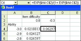
• Step 1 In EXCEL, create a spreadsheet with the first column showing abilities from −3 to 3, in steps of 0.1. In Cell B2, type in a value for an item difficulty, say 0.8, as shown below.

  

• Step 2 In Cell B4, compute the probability of success: Type the following formula, as shown

  $$ = \exp \left( {\$ A 4- B\$ 2} \right)/\left( { 1+ \exp \left( {\$ A 4- B\$ 2} \right)} \right) $$
  

• Step 3 Autofill the rest of column B, for all ability values, as shown

  

• Step 4 Make a XY (scatter) plot of ability against probability of success, as shown below.

  

  This graph shows the probability of success (Y axis) against ability (X axis), for an item with difficulty 0.8.

• Q1. When the ability equals the item difficulty (0.8 in this case), what is the probability of success?

• Step 5 Add another item in the spreadsheet with item difficulty of −0.3. In Cell C2, enter −0.3. Autofill cell C4 from cell B4. Then autofill the column of C for the other ability values.

  

• Step 6 Plot the probability of success on both items, as a function of ability (hint: plot columns A, B and C).

  

• Q2. A person with ability −1.0 has a probability of 0.14185 of getting the first item right. At what ability does a person have the same probability of getting the second item right?

• Q3. What is the difference between the abilities of the two persons where Person A’s probability of getting the first item right is the same as Person B’s probability of getting the second item right?

• Q4. How does this difference relate to the item difficulties of the two items?

• Q5. If there is a very difficult item (say, with difficulty value of 2), can you sketch the probability curves on the above graph (without computing it in EXCEL)? Check your graph with an actual computation and plot in EXCEL.

Task 2. Compare Logistic and Normal Ogive Functions

The following shows an excerpt of an EXCEL spreadsheet.

In column A, set a sequence of abilities from −3 to 3, in steps of 0.1.

In column B, compute the logistic function

$$ \frac{{\exp \left( {\theta - \delta } \right)}}{{1 + \exp \left( {\theta - \delta } \right)}} $$

where $\theta$ is the person-parameter (ability in column A) and $\delta$ is zero. More specifically, type the formula “=exp(A2)/(1 + exp(A2))” in cell B2, and auto-fill column B.

In column C, compute the normal ogive function (i.e., cumulative normal distribution with mean 0 and standard deviation 1). Specifically, in column C2, type the formula “=normdist(A2, 0, 1, 1)”.

In column D, compute the logistic function, but this time, use a scale parameter of 1.7. Specifically, in cell D2, type the formula “=exp(1.7 * A2)/(1 + exp(1.7 * A2))”.

Make a scatter plot of columns A to D on the same graph. You should get a graph like the following:

Which two functions overlap with each other?

Since the ability scale has an arbitrary scale factor, it does not matter whether we use $\frac{{\exp \left( {\theta - \delta } \right)}}{{1 + \exp \left( {\theta - \delta } \right)}}$ or $\frac{{\exp \left( {1.7\left( {\theta - \delta } \right)} \right)}}{{1 + \exp \left( {1.7\left( {\theta - \delta } \right)} \right)}}$.

The latter form is still a Rasch model, and it is very close to the normal ogive function. For this reason, some software programs set the ability scale with a scale factor of 1.7 instead of 1. This will not affect the interpretations of IRT results in any way.

Task 3. Compute the Likelihood Function

To understand the idea of raw score as sufficient statistic for ability estimate, this hands-on practice shows the comparison between likelihood functions for different item response patterns with the same raw test score.

We will use EXCEL for this exercise. Figure 7.10 shows an EXCEL spreadsheet.

Fig. 7.10

Computation of likelihood function

In this example, a test has five items where the item difficulties are −2, −1, 0, 1 and 2 (see Row 2 in the spreadsheet in Fig. 7.10). In cells A5 to A17, there is a list of abilities from −3 to 3. Row 3 contains an item response pattern. In this example, it is assumed that a student obtained a score of three by answering Items 1, 3 and 5 correctly. In cells B5 to F17, compute the probability of the item response with given ability. The EXCEL formula in B5 is “=EXP(B$3 * ($A5 − B$2))/(1 + EXP($A5 − B$2))”. The multiplier “B$3” in the formula is the item response. This formula evaluates to $\frac{{\exp \left( {\theta - \delta_{i} } \right)}}{{1 + \exp \left( {\theta - \delta_{i} } \right)}}$ when the item response is 1, and $\frac{1}{{1 + \exp \left( {\theta - \delta_{i} } \right)}}$ when the item response is 0. Column G is the likelihood which is the product of the probabilities in cells B to F.

Scanning down column G, the largest value (maximum) is in row 12, when the ability is 0.5. This is the ability that “maximises” the likelihood. So the ability estimate for a response pattern of “10101” (right-wrong-right-wrong-right) will be around 0.5.

Repeat this computation for a different response pattern but still for a raw score of 3. For example, use the response pattern “01101” in cells B3 to F3. What is the maximum likelihood and which ability corresponds to this maximum likelihood?

Plot the likelihood functions for both response patterns “10101” and “01101” as a function of ability. Figure 7.11 shows such a graph.

Fig. 7.11

Likelihood as a function of ability and item response pattern

Repeat this for another response pattern, say, “11100”, and plot the likelihood for the three response patterns on the same graph.

Discussion Points

• 1. In relation to the Hands-on Practices Task 3, discuss the concept of “raw score as sufficient statistic for ability estimate”. For example, given a raw score, how do different response patterns affect the estimation of ability? Given a raw score, compare the likelihood functions for similarities and differences for different response patterns. Would different response patterns impact on the fit of the items to the model?

• 2. From a fairness point of view, do you think the ability estimate should be the same for the same raw score irrespective of the actual items answered correctly? If not, how would you score the items? Consider the illustrative example. If Items 9 and 10 are administered, one student got Item 9 right but Item 10 wrong, the other student got Item 9 wrong but Item 10 right, so both students got 1 out of 2. Should they have the same ability estimate?

• 3. Discuss the concept of “sample-free” in Rasch models. In what ways are estimated statistics sample-free and sample-dependent?