Conclusion of Volume 2

Abstract

This final short chapter summarizes the logical and historical development told in the two Volumes from the first intuition of Lorentz invariance to the current frontier of research in Gravity Theory. The conclusive hope of the author is spelled out. He will be satisfied if his reader has strengthened his belief in that the Universe is Gravitation, Gravitation is Geometry but Geometry is enormously variegated and full of yet undiscovered surprises.

Appendices

This appendix is present also in Volume 1. It is repeated in Volume 2 for reader’s convenience.

Appendix A: Spinors and Gamma Matrix Algebra

This appendix is present also in Volume 1. It is repeated in Volume 2 for reader’s convenience.

10.1.1 A.1 Introduction to the Spinor Representations of SO(1,D−1)

The spinor representations of the orthogonal and pseudo-orthogonal groups have different structure in various dimensions. Starting from the representation of the Dirac gamma matrices one begins with a complex representation whose dimension is equal to the dimension of the gammas. A vector in this complex linear space is named a Dirac spinor. Typically Dirac spinors do not form irreducible representations. Depending on the dimensions, one can still impose SO(1,D−1) invariant conditions on the Dirac spinor that separate it into irreducible parts. These constraints can be of two types:

• (a) A reality condition which maintains the number of components of the spinor but relates them to their complex conjugates by means of linear relations. This reality condition is constructed with an invariant matrix $\mathcal{C}$, named the charge conjugation matrix whose properties depend on the dimensions D.

• (b) A chirality condition constructed with a chirality matrix Γ _D+1 that halves the number of components of the spinor. The chirality matrix exists only in even dimensions.

Depending on which conditions can be imposed, besides Dirac spinors, in various dimensions D, one has Majorana spinors, Weyl spinors and, in certain dimensions, also Majorana-Weyl spinors. In this appendix we discuss the properties of gamma matrices and we present the various types of irreducible spinor representations in all relevant dimensions from D=4 to D=11. The upper bound D=11 is dictated by supersymmetry since supergravity, i.e. the supersymmetric extension of Einstein gravity, can be constructed in all dimensions up to D=11, which is maximal in this respect.

10.1.2 A.2 The Clifford Algebra

In order to describe spinors one needs the Dirac gamma matrices. These form the Clifford algebra:

$$ \{ \varGamma_a , \varGamma_b\} = 2 \eta_{ab} $$

(A.2.1)

where η _ab is the invariant metric of SO(1,D−1), that we always choose according to the mostly minus conventions, namely:

$$ \eta_{ab} = \mbox{diag}( +,-,-,\ldots,-) $$

(A.2.2)

To study the general properties of the Clifford algebra (A.2.1) we use a direct construction method.

We begin by fixing the following conventions. Γ ⁰=Γ ₀ corresponding to the time direction is Hermitian:

$$ \varGamma^\dagger_0 = \varGamma_0 $$

(A.2.3)

while the matrices Γ _i =−Γ ⁱ corresponding to space directions are anti-Hermitian:

$$ \varGamma^\dagger_i = - \varGamma_i $$

(A.2.4)

In the study of Clifford algebras it is necessary to distinguish the case of even and odd dimensions.

10.1.2.1 A.2.1 Even Dimensions

When D=2ν is an even number the representation of the Clifford algebra (A.2.1) has dimension:

$$ \operatorname{dim}\varGamma_a = 2^{\frac{D}{2}} = 2^\nu $$

(A.2.5)

In other words the gamma matrices are 2^ν×2^ν. The proof of such a statement is easily obtained by iteration. Suppose that we have the gamma matrices γ _a corresponding to the case ν′=ν−1, satisfying the Clifford algebra (A.2.1) in D−2 dimensions and that they are 2^ν′-dimensional. We can write down the following representation for the gamma matrices in D-dimension by means of the following 2^ν×2^ν matrices:

(A.2.6)

which satisfy the correct anticommutation relations and have the correct hermiticity properties specified above. This representation admits the following interpretation in terms of matrix tensor products:

$$ \varGamma_{a^\prime} = \gamma_{a^\prime} \otimes \sigma_1 ; \qquad \varGamma_{D-2} = \mathbf{1}\otimes{ \mathrm{i}} \sigma_3 ;\qquad \varGamma_{D-1} = \mathbf{1} \otimes{\mathrm{i}} \sigma_2 $$

(A.2.7)

where σ _1,2,3 denote the Pauli matrices:

$$ \sigma_1 = \left ( \begin{array}{c@{\quad}c} 0 & 1 \\ 1 & 0 \end{array} \right ) ;\qquad \sigma_2 = \left ( \begin{array}{c@{\quad}c} 0 & -{\mathrm{i}} \\ {\mathrm{i}} & 0 \end{array} \right ) ;\qquad \sigma_3 = \left ( \begin{array}{c@{\quad}c} 1 & 0 \\ 0 & - 1 \end{array} \right ) $$

(A.2.8)

To complete the proof of our statement we just have to show that for ν=2, corresponding to D=4 we have a 4-dimensional representation of the gamma matrices. This is well established. For instance we have the representation:

(A.2.9)

In D=2ν one can construct the chirality matrix defined as follows:

$$ \varGamma_{D+1} = \alpha_D \varGamma_0 \varGamma_1 \varGamma_2 \ldots \varGamma_{D-1} ; \qquad|\alpha_D|^2 = 1 $$

(A.2.10)

where α _D is a phase-factor to be fixed in such a way that:

$$ \varGamma^2_{D+1} = \mathbf{1} $$

(A.2.11)

By direct evaluation one can verify that:

$$ \{ \varGamma_a , \varGamma_{D+1} \} = 0 \quad a = 0,1,2,\ldots , D-1 $$

(A.2.12)

The normalization α _D is easily derived. We have:

$$ \varGamma_0 \varGamma_1 \ldots \varGamma_{D-1} = ( -)^{\frac {1}{2} D(D-1)} \varGamma_{D-1} \varGamma_{D-2} \varGamma_{D-1} $$

(A.2.13)

so that imposing (A.2.11) results into the following equation for α _D :

$$ \alpha^2_D ( -)^{\frac {1}{2} D(D-1)} ( -)^{(D-1)} = 1 $$

(A.2.14)

which has solution:

$$ \begin{array}{cc@{\quad}l} \alpha_D & = 1 &\mbox{if } \nu = 2\mu+1 \sim\mbox{odd} \\[2pt] \alpha_D & = {\mathrm{i}}& \mbox{if } \nu = 2\mu \sim \mbox{even} \end{array} $$

(A.2.15)

With the same token we can show that the chirality matrix is Hermitian:

$$ \varGamma_{D+1}^\dagger = \alpha^\star ( -)^{\frac {1}{2} D(D-1)} ( -)^{(D-1)} \varGamma_0 \varGamma_1 \varGamma_2 \ldots \varGamma_{D-1} = \varGamma_{D+1} $$

(A.2.16)

10.1.2.2 A.2.2 Odd Dimensions

When D=2ν+1 is an odd number, the Clifford algebra (A.2.1) can be represented by 2^ν×2^ν matrices. It suffices to take the matrices Γ _a′ corresponding to the even case D′=D−1 and add to them the matrix Γ _D =iΓ _D′+1, which is anti-Hermitian and anti-commutes with all the other ones.

10.1.3 A.3 The Charge Conjugation Matrix

Since Γ _a and their transposed $\varGamma_{a}^{T}$ satisfy the same Clifford algebras it follows that there must be a similarity transformation connecting these two representations of the same algebra on the same carrier space. Such statement relies on Schur’s lemma and it is proved in the following way. We introduce the notation:

$$ \varGamma_{a_1\dots a_n} \equiv \varGamma_{[a_1} \varGamma_{a_2} \dots \varGamma_{a_n]} = \frac{1}{n!} \sum _{P} (-)^{\delta_{P}} \varGamma_{a_{P(a_1)}} \ldots \varGamma_{a_{P(a_n)}} $$

(A.3.1)

where ∑ _P denotes the sum over the n! permutations of the indices and δ _P the parity of permutation P, i.e. the number of elementary transpositions of which it is composed. The set of all matrices $1, \varGamma_{a} , \varGamma_{a_{1}a_{2}}, \ldots,\varGamma_{a_{1} \ldots a_{D}}$ constitutes a finite group of 2^[D/2]-dimensional matrices. Furthermore the groups generated in this way by Γ _a , −Γ _a or $\varGamma_{a}^{T}$ are isomorphic. Hence by Schur’s lemma two irreducible representations of the same group, with the same dimension and defined over the same vector space, must be equivalent, that is there must be a similarity transformation that connects the two. The matrix realizing such a similarity is called the charge conjugation matrix. Instructed by this discussion we define the charge conjugation matrix by means of the following equations:

(A.3.2)

By definition ${{\mathcal{C}}_{\pm }}$ connects the representation generated by Γ _a to that generated by $\pm \varGamma_{a}^{T}$. In even dimensions both ${{\mathcal{C}}_{-}}$ and ${{\mathcal{C}}_{+}}$ exist, while in odd dimensions only one of the two is possible. Indeed in odd dimensions Γ _D−1 is proportional to Γ ₀ Γ ₁…Γ _D−2 so that the ${{\mathcal{C}}_{-}}$ and ${{\mathcal{C}}_{+}}$ of D−1 dimensions yield the same result on Γ _D−1. This decides which $\mathcal{C}$ exists in a given odd dimension.

Another important property of the charge conjugation matrix follows from iterating (A.3.2). Using Schur’s lemma one concludes that ${{\mathcal{C}}_{\pm }}=\alpha \mathcal{C}_{\pm }^{T}$ so that iterating again we obtain α ²=1. In other words ${{\mathcal{C}}_{+}}$ and ${{\mathcal{C}}_{-}}$ are either symmetric or antisymmetric. We do not dwell on the derivation which can be obtained by explicit iterative construction of the gamma matrices in all dimensions and we simply collect below the results for the properties of ${{\mathcal{C}}_{\pm }}$ in the various relevant dimensions (see Table A.1).

Table A.1 Structure of charge conjugation matrices in various space-time dimensions

10.1.4 A.4 Majorana, Weyl and Majorana-Weyl Spinors

The Dirac conjugate of a spinor ψ is defined by the following operation:

$$ \overline {\psi} \equiv \psi^\dagger \varGamma_0 $$

(A.4.1)

and the charge conjugate of ψ is defined as:

$$ {{\psi }^{c}}=\mathcal{C}_{\psi }^{-T} $$

(A.4.2)

where $\mathcal{C}$ is the charge conjugation matrix. When we have such an option we can either choose ${{\mathcal{C}}_{+}}$ or ${{\mathcal{C}}_{-}}$. By definition a Majorana spinor λ satisfies the following condition:

$$ \lambda = \lambda^c = C \varGamma_0^T \lambda^\star $$

(A.4.3)

Equation (A.4.3) is not always self-consistent. By iterating it a second time we get the consistency condition:

$$ \mathcal{C}\Gamma _{0}^{T}\mathcal{C}={{\Gamma }_{0}} $$

(A.4.4)

There are two possible solutions to this constraint. Either ${{\mathcal{C}}_{-}}$ is antisymmetric or ${{\mathcal{C}}_{+}}$ is symmetric. Hence, in view of the results displayed above, Majorana spinors exist only in

$$ D = 4,8,9,10,11 $$

(A.4.5)

In D=4,10,11 they are defined using the ${{\mathcal{C}}_{-}}$ charge conjugation matrix while in D=8,9 they are defined using ${{\mathcal{C}}_{+}}$.

Weyl spinors, on the contrary, exist in every even dimension; by definition they are the eigenstates of the Γ _D+1 matrix, corresponding to the +1 or −1 eigenvalue. Conventionally the former eigenstates are named left-handed, while the latter are named right-handed spinors:

$$ {{\Gamma }_{D+1}}{{\psi }_{\left( \begin{matrix} L \\ R \\\end{matrix} \right)}}=\pm {{\psi }_{\left( \begin{matrix} L \\ R \\\end{matrix} \right)}} $$

(A.4.6)

In some special dimensions we can define Majorana-Weyl spinors which are both eigenstates of Γ _D+1 and satisfy the Majorana condition (A.4.3). In order for this to be possible we must have:

$$ \mathcal{C}\Gamma _{0}^{T}\Gamma _{D+1}^{\bigstar }{{\psi }^{\bigstar }}={{\Gamma }_{D+1}}\psi $$

(A.4.7)

which implies:

$$ \mathcal{C}\Gamma _{0}^{T}\Gamma _{D+1}^{\bigstar }\Gamma _{0}^{T}{{\mathcal{C}}^{-1}}={{\Gamma }_{D+1}} $$

(A.4.8)

With some manipulations the above condition becomes:

$$ \mathcal{C}{{\Gamma }_{D+1}}{{\mathcal{C}}^{-1}}=-\Gamma _{D+1}^{T} $$

(A.4.9)

which can be checked case by case, using the definition of Γ _D+1 as product of all the other gamma matrices. In the range 4≤D≤11 the only dimension where (A.4.9) is satisfied is D=10 which is the critical dimensions for superstrings. This is not a pure coincidence.

Summarizing we have:

Spinors in 4≤D≤11
D	Dirac	Majorana	Weyl	Majora-Weyl
4	Yes	Yes	Yes	No
5	Yes	No	No	No
6	Yes	No	Yes	No
7	Yes	No	No	No
8	Yes	Yes	Yes	No
9	Yes	Yes	No	No
10	Yes	Yes	Yes	Yes
11	Yes	Yes	No	No

10.1.5 A.5 A Particularly Useful Basis for D=4 γ-Matrices

In this section we construct a D=4 gamma matrix basis which is convenient for various purposes. Let us first specify the basis and then discuss its convenient properties.

In terms of the standard matrices (A.2.8) we realize the $\mathfrak {so}(1,3)$ Clifford algebra:

$$ \{ \gamma_a , \gamma_b \} = 2 \eta_{ab} ; \qquad\eta_{ab} = \mbox{diag} ( + , - , - , - ) $$

(A.5.1)

by setting:

(A.5.2)

where γ ₅ is the chirality matrix and $\mathcal{C}$ is the charge conjugation matrix. In this basis the generators of the Lorentz algebra $\mathfrak {so}(1,3)$, namely γ _ab are particularly simple and nice 4×4 matrices. Explicitly we get:

(A.5.3)

Let us mention some relevant formulae that are easily verified in the above basis:

$$ \gamma_0\gamma_1 \gamma_2 \gamma_3 = {\mathrm{i}} \gamma_5 $$

(A.5.4)

and if we fix the convention:

$$ \varepsilon _{0123} = + 1 $$

(A.5.5)

we obtain:

$$ \frac {1}{24} \varepsilon ^{\mathit{abcd}} \gamma_a \gamma_b \gamma_c \gamma_d = - {\mathrm{i}} \gamma_5 $$

(A.5.6)

Appendix B: Auxiliary Tools for p-Brane Actions

In this appendix we collect some auxiliary calculations and algebraic tools relevant to the discussion of p-brane world volume actions presented in Chap. 7.

10.1.1 B.1 Notations and Conventions

General adopted notations for first order world volume actions are the following ones:

(B.1.1)

10.1.2 B.2 The κ-Supersymmetry Projector for D3-Branes

In this appendix we present the derivation of the κ-supersymmetry projector utilized in Sect. 7.5 to establish the κ-susy invariance of the D3-brane action. In particular we refer to (7.5.23).

Let us begin with property (a) and consider the ansatz in (7.5.26). By direct calculation we find:

$$ \begin{array}{rcl} \omega_{[4]}^{2} & = & \alpha_{4}^{2} (4!)^{2}\\[8pt] \omega_{[2]}^{2} & = & \dfrac{(\alpha_{2})^{2} \omega_{[0]} \omega_{[4]} }{3! \alpha_{0} \alpha_{4} } + 8 (\alpha_{2})^{2} \operatorname{Tr}\bigl(\widehat{F}^{\,2}\bigr) \end{array} $$

(B.2.1)

so that we get:

$$ \varGamma^{2} = \frac{1}{N^{2}} \biggl[ (4! \alpha_4)^2 + \omega_{[0]} \omega_{[4]} \biggl(\frac{(\alpha_2)^{2}}{3!\alpha_0 \alpha_4} + 2 \biggr) + 8(\alpha_2)^2 \operatorname{Tr}\bigl( \widehat{F}^2\bigr) \biggr] $$

(B.2.2)

so we obtain Γ ²=1 if the normalization factor N is chosen as in (7.5.27) and if the coefficients are chosen as in (7.5.28). This conclusion is easily reached using the identity (7.5.30) of the main text.

Let us now turn to property (b), namely to the condition

$$ \varGamma A_{k} = A_{k} $$

(B.2.3)

To implement it we need to calculate some γ matrix products:

$$ \begin{array}{rcl} \omega_{[4]} \gamma_{k} & = & \dfrac{1}{6} \tilde{ \gamma}_{k} \\[8pt] \omega_{[4]} \tilde{\gamma}_{k} & = & 6 \gamma_{k} \\[8pt] \omega_{[4]} \varPi_{k} & = & - \dfrac{1}{2} \skew{1}\widetilde{ \widehat {F}}^{\,ij}\gamma_{ijk} \equiv- \dfrac{1}{2} \widetilde{ \varDelta }_{k} \\[8pt] \omega_{[4]} \widetilde{\varPi}_{k} & = & - \dfrac{1}{2} \widehat{F}^{ij}\gamma_{ijk} \equiv- \dfrac{1}{2} \varDelta _{k} \end{array} $$

(B.2.4)

$$ \begin{array}{rcl} \omega_{[2]} \gamma_{k} & = & \dfrac{i}{2} \widetilde{ \varDelta }_{k} + i \widetilde{\varPi}_{k} \\[8pt] \omega_{[2]} \tilde{\gamma}_{k} & = & - 3 i \varDelta _{k} - 6 i \varPi_{k} \\[8pt] \omega_{[2]} \varPi_{k} & = & - \dfrac{i}{6} \bigl( \widehat{F}^{\,2}\bigr)_{kl} \tilde{\gamma}^{l} - i \omega_{[0]} \gamma_{k} \\[8pt] \omega_{[2]} \widetilde{\varPi}_{k} & = & i \bigl(\skew{1}\widetilde{ \widehat{F}}^{\,2}\bigr)_{kl} \gamma^{l} + \dfrac{i}{6} \omega_{[0]} \tilde{\gamma}_{k} \end{array} $$

(B.2.5)

Now we impose (B.2.3) and we obtain the following equations.

• The contributions from Δ _k and $\widetilde{\varDelta }_{k}$ are:

  $$ \begin{array}{rcl} \varDelta ^{m} h_{mk} \biggl(\dfrac{i}{2} f_{4} + 3 f_{2}\biggr) \otimes \sigma_{1} & = & 0 \\[14pt] \widetilde{\varDelta }_{k} \biggl( - \dfrac{i}{2} f_{3} + \dfrac{i}{2} f_{1} \biggr) \otimes\sigma_{2} & = & 0 \end{array} $$

  (B.2.6)

• For the contributions with γ _k we have two equations, one proportional to σ ₃ and one proportional to 1, namely:

  $$ \gamma_{k} \omega_{[0]} ( f_{1} - f_{3} ) \otimes\sigma_{3} = 0 $$

  (B.2.7)

  and

  $$ \frac{1}{N}(6{{f}_{2}}{{\mathbf{1}}_{4\times 4}}+i{{f}_{4}}{{\tilde{\hat{F}}}^{2}})h\otimes {{\mathbf{1}}_{2\times 2}}=\text{i}{{f}_{1}}{{\mathbf{1}}_{4\times 4}}\otimes {{\mathbf{1}}_{2\times 2}} $$

  (B.2.8)

  For:

  $$ \begin{array}{rcl} 6 f_{2} = \mathrm{i}f_1 \\[6pt] \mathrm{i} f_1 = -i f_4 \end{array} $$

  (B.2.9)

  and using the property (7.5.31) we obtain:

  

  (B.2.10)

• For the contributions with $\tilde{\gamma}_{k}$ we get the following equations:

  $$ \begin{array}{rcl} \tilde{\gamma}_{m} h^{m}_{\phantom{m}k} \omega_{[0]} \biggl( f_{2} + \dfrac{i}{6} f_4 \biggr) \otimes\mathbf{1}_{2 \times2} & = & 0 \\[14pt] N^{-1} \tilde{\gamma}_{m} \biggl[ \dfrac{1}{6} f_1 \delta^{m}_{\phantom{m}k} -\dfrac{1}{6} f_3 \bigl(\widehat{F}^{\,2}\bigr)^{m}_{\phantom{m}k} \biggr] \otimes\sigma_3 & = & f_2 \tilde{ \gamma}_{m} h^{m}_{\phantom{m}k} \otimes \sigma_3 \end{array} $$

  (B.2.11)

  Then if:

  

  (B.2.12)

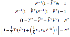
  we obtain that the second of equations (B.2.11) as a matrix equation becomes:

  $$ {{N}^{-1}}[\mathbf{1}-({{\hat{F}}^{2}})]=h $$

  (B.2.13)

  and just coincides with the solution (7.4.51) for the auxiliary field h in terms of the physical ones.

• Now we consider Π and $\widetilde{\varPi}$.

  The equation proportional to σ ₁ is:

  $$ \begin{array}{rcl} \alpha \omega_{[0]} \widetilde{\varPi}^{m} h_{mk} + \beta \varPi^{m} h_{mk} & = & N \gamma \varPi^{k} \\[8pt] \alpha \omega_{[0]} \skew{1}\widetilde{\widehat{F}}^{\,lm} h_{mk} \gamma_{l} + \beta\widehat{F}^{\,lm} h_{mk} \gamma_{l} & = & \gamma N \widehat{F}^{\,l}_{\phantom{\,l}k}\, \gamma_{l} \end{array} $$

  (B.2.14)

  in matrix form we have:

  

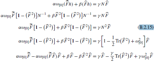  (B.2.15)

  if:

  $$ \beta =\gamma $$

  (B.2.16)

  and using (7.5.31), than (B.2.15) become:

  $$ \alpha {{\omega }_{[0]}}\tilde{\hat{F}}-\alpha \omega _{[0]}^{2}\hat{F}-\beta {{\hat{F}}^{2}}\hat{F}=-\frac{\gamma }{2}\text{Tr(}{{\hat{F}}^{2}}\text{)}\hat{F}+\gamma \omega _{[0]}^{2}\hat{F} $$

  (B.2.17)

  if:

  $$ \alpha =\gamma $$

  (B.2.18)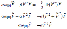
  

  (B.2.19)

  and it is correct by (7.5.31).

  The equation proportional to σ ₂ is:

  

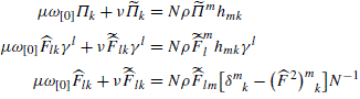  (B.2.20)

  for:

  $$ \begin{array}{rcl} \nu&=& \rho \\[4pt] \mu&=& \rho \end{array} $$

  (B.2.21)

  we obtain the first of the relations (7.5.31).

  Where:

  $$ \begin{array}{rcl@{\qquad }rcl@{\qquad }rcl} \alpha&=& -{i} f_{4} & \beta&=& 6 {i} f_{2} & \gamma&=& f_{3} \\[6pt] \mu&=& {i} f_{3} & \nu&= &{i} f_{1} & \rho&=& f_{4} \end{array} $$

  (B.2.22)

  Using the fact that $a_{5}= \frac{3}{4}$ and (7.5.18) we have that (B.2.6), (B.2.7), (B.2.9), (B.2.12), and (B.2.16), (B.2.18), (B.2.21) are automatically satisfied. This concludes the proof of property (b) and hence of κ supersymmetry.

Appendix C: Auxiliary Information About Some Superalgebras

10.1.1 C.1 The OSp$(\mathcal{N}\mathbf{|4})$ Supergroup, Its Superalgebra and Its Supercosets

In this appendix we provide some explicit information and a collection of very useful formulae relative to the very important class of supergroups OSp$(\mathcal{N}\text{ }\!\!|\!\!\text{ 4})$ which appears in the compactification of superstrings and of M-theory on anti de Sitter backgrounds. The presented material closely follows two sections of paper [1].

10.1.1.1 C.1.1 The Superalgebra

The real form $\mathfrak{o}\mathfrak{s}\mathfrak{p}(\mathcal{N}|4)$ of the complex $\mathfrak{o}\mathfrak{s}\mathfrak{p}(\mathcal{N}|4,\mathbb{C})$ Lie superalgebra which is relevant for the study of $\text{Ad}{{\text{S}}_{4}}\times \mathcal{G}|\mathcal{H}$ compactifications is that one where the ordinary Lie subalgebra is the following:

$$ \mathfrak{s}\mathfrak{p}\text{(4,}\mathbb{R}\text{)}\times \mathfrak{s}\mathfrak{o}\text{(}\mathcal{N}\text{)}\subset \mathfrak{o}\mathfrak{s}\mathfrak{p}\text{(}\mathcal{N}\text{ }\!\!|\!\!\text{ 4)} $$

(C.1.1)

This is quite obvious because of the isomorphism $\mathfrak {sp}(4,\mathbb{R}) \simeq \mathfrak {so}(2,3)$ which identifies $\mathfrak {sp}(4,\mathbb{R})$ with the isometry algebra of anti de Sitter space. The compact algebra $\mathfrak{s}\mathfrak{o}\text{(}\mathcal{N}\text{)}$ is instead the R-symmetry algebra acting on the supersymmetry charges.

The superalgebra $\mathfrak{o}\mathfrak{s}\mathfrak{p}\text{(}\mathcal{N}\text{ }\!\!|\!\!\text{ 4)}$ can be introduced as follows: consider the two graded $(4+\mathcal{N})\times (4+\mathcal{N})$ matrices:

(C.1.2)

where C is the charge conjugation matrix in D=4. The matrix $\widehat{C}$ has the property that its upper block is antisymmetric while its lower one is symmetric. On the other hand, the matrix $\widehat{H}$ has the property that both its upper and lower blocks are Hermitian. The $\mathfrak{o}\mathfrak{s}\mathfrak{p}\text{(}\mathcal{N}\text{ }\!\!|\!\!\text{ 4)}$ Lie algebra is then defined as the set of graded matrices Λ satisfying the two conditions:

$$ {{\Lambda }^{T}}\hat{C}+\hat{C}\Lambda =0 $$

(C.1.3)

$$ {{\Lambda }^{\dagger }}\hat{H}+\hat{H}\Lambda =0 $$

(C.1.4)

Equation (C.1.3) defines the complex $\mathfrak{o}\mathfrak{s}\mathfrak{p}\text{(}\mathcal{N}\text{ }\!\!|\!\!\text{ 4)}$ superalgebra while (C.1.4) restricts it to the appropriate real section where the ordinary Lie subalgebra is (C.1.1). The specific form of the matrices $\widehat{C}$ and $\widehat{H}$ is chosen in such a way that the complete solution of the constraints (C.1.3), (C.1.4) takes the following form:

(C.1.5)

and the Maurer-Cartan equations

$$ d \varLambda + \varLambda \wedge \varLambda = 0 $$

(C.1.6)

read as follows:

(C.1.7)

Interpreting E ^a as the vielbein, ω ^ab as the spin connection, and ψ ^a as the gravitino 1-form, (C.1.7) can be viewed as the structural equations of a supermanifold $\text{Ad}{{\text{S}}_{4|\mathcal{N}\times 4}}$ extending anti de Sitter space with $\mathcal{N}$ Majorana supersymmetries. Indeed the gravitino 1-form is a Majorana spinor since, by construction, it satisfies the reality condition

$$ C \overline{\psi}_A^T = \psi_A , \qquad \overline{\psi }_A \equiv \psi_A^\dagger \gamma_0 $$

(C.1.8)

The supermanifold $\text{Ad}{{\text{S}}_{4|\mathcal{N}\times 4}}$ can be identified with the following supercoset:

$$ \mathcal{M}_{\text{osp}}^{4|4\mathcal{N}}=\frac{\text{Osp}(\mathcal{N}|4)}{\text{SO}(\mathcal{N})\times \text{SO}(1,3)} $$

(C.1.9)

Alternatively, the Maurer Cartan equations can be written in the following more compact form:

(C.1.10)

where all 1-forms are real and, according to our conventions, the indices x, y, z, t are symplectic and take four values. The real symmetric bosonic 1-form Ω ^xy=Ω ^yx encodes the generators of the Lie subalgebra $\mathfrak {sp}(4,\mathbb{R})$, while the antisymmetric real bosonic 1-form ${{\Omega }^{xy}}={{\Omega }^{yx}}$ encodes the generators of the Lie subalgebra $\mathfrak{s}\mathfrak{o}(\mathcal{N})$. The fermionic 1-forms $\varPhi^{x}_{A}$ are real and, as indicated by their indices, they transform in the fundamental 4-dim representation of $\mathfrak {sp}(4,\mathbb{R})$ and in the fundamental $\mathcal{N}$-dim representation of $\mathfrak{s}\mathfrak{o}(\mathcal{N})$. Finally,

$$ {{\varepsilon }_{xy}}=-{{\varepsilon }_{yx}}=\left( \begin{matrix} 0 & 0 & 0 & 1 \\ 0 & 0 & -1 & 0 \\ 0 & 1 & 0 & 0 \\ -1 & 0 & 0 & 0 \\\end{matrix} \right) $$

(C.1.11)

is the symplectic invariant metric.

The relation between the formulation (C.1.7) and (C.1.10) of the same Maurer Cartan equations is provided by the Majorana basis of d=4 gamma matrices discussed in Appendix C.3.2. Using (A.5.2), the generators γ _ab and γ _a γ ₅ of the anti de Sitter group SO(2,3) turn out to be all given by real symplectic matrices, as is explicitly shown in (A.5.3) and the matrix $\mathcal{C}{{\gamma }_{5}}$ turns out to be proportional to ε _xy as shown in (C.3.7). On the other hand a Majorana spinor in this basis is proportional to a real object times a phase factor exp[−πi/4].

Hence (C.1.7) and (C.1.10) are turned ones into the others upon the identifications:

(C.1.12)

As it is always the case, the Maurer Cartan equations are just a property of the (super) Lie algebra and hold true independently of the (super) manifold on which the 1-forms are realized: on the supergroup manifold or on different supercosets of the same supergroup.

10.1.2 C.2 The Relevant Supercosets and Their Relation

Let us also consider the following pure fermionic coset:

$$ \mathcal{M}_{\text{osp}}^{0|4\mathcal{N}}=\frac{\text{Osp}(\mathcal{N}|4)}{\text{SO}(\mathcal{N})\times \text{Sp}(4,\mathbb{R})} $$

(C.2.1)

There is an obvious relation between these two supercosets that can be formulated in the following way:

$$ \mathcal{M}_{\text{osp}}^{0|4\mathcal{N}}\tilde{\ }\text{Ad}{{\text{S}}_{4}}\times \mathcal{M}_{\text{osp}}^{0|4\mathcal{N}} $$

(C.2.2)

In order to explain the actual meaning of (C.2.2) we proceed as follows. Let the graded matrix $\mathbb{L}\in \text{Osp(}\mathcal{N}\text{ }\!\!|\!\!\text{ 4)}$ be the coset representative of the coset $\mathcal{M}_{\text{osp}}^{4|4\mathcal{N}}$, such that the Maurer Cartan form Λ of (C.1.5) can be identified as:

$$ \varLambda= \mathbb{L}^{-1} \, d \mathbb{L} $$

(C.2.3)

Let us now factorize $\mathbb{L}$ as follows:

$$ \mathbb{L} = \mathbb{L}_F \mathbb{L}_B $$

(C.2.4)

where $\mathbb{L}_{F}$ is a coset representative for the coset:

$$ \frac{\text{Osp}(\mathcal{N}|4)}{\text{SO}(\mathcal{N})\times \text{Sp}(4,\mathbb{R})}\backepsilon {{\mathbb{L}}_{F}} $$

(C.2.5)

and $\mathbb{L}_{B}$ is the $\text{Osp(}\mathcal{N}\text{ }\!\!|\!\!\text{ 4)}$ embedding of a coset representative of AdS₄, namely:

(C.2.6)

In this way we find:

$$ \varLambda= \mathbb{L}_B^{-1} \varLambda_F \mathbb{L}_B + \mathbb{L}_B^{-1} \, d \mathbb{L}_B $$

(C.2.7)

Let us now write the explicit form of Λ _F in analogy to (C.1.5):

(C.2.8)

where Θ _A is a Majorana-spinor valued fermionic 1-form and where Δ _F is an $\mathfrak {sp}(4,\mathbb{R})$ Lie algebra valued 1-form presented as a 4×4 matrix. Both Θ _A as Δ _F and ${{\tilde{\mathcal{A}}}_{AB}}$ depend only on the fermionic θ coordinates and differentials.

On the other hand we have:

(C.2.9)

where the Ω _B is also an $\mathfrak {sp}(4,\mathbb{R})$ Lie algebra valued 1-form presented as a 4×4 matrix, but it depends only on the bosonic coordinates x ^μ of the anti de Sitter space AdS₄. Indeed, according to (C.1.5) we can write:

$$ \varDelta _B = - \frac {1}{4} B^{ab} \gamma_{ab} - 2 e \gamma_a \gamma_5 B^a $$

(C.2.10)

where {B ^ab,B ^a} are respectively the spin-connection and the vielbein of AdS₄, just as $\{{{\mathcal{B}}^{\alpha \beta }},{{\mathcal{B}}^{\alpha }}\}$ are the connection and vielbein of the internal coset manifold $\mathcal{M}{{}_{7}}$.

Inserting now these results into (C.2.7) and comparing with (C.1.5) we obtain:

(C.2.11)

The above formulae encode an important information. They show how the supervielbein and the superconnection of the supermanifold (C.1.9) can be constructed starting from the vielbein and connection of AdS₄ space plus the Maurer Cartan forms of the purely fermionic supercoset (C.2.1). In other words formulae (C.2.11) provide the concrete interpretation of the direct product (C.2.2). This will also be our starting point for the actual construction of the supergauge completion in the case of maximal supersymmetry and for its generalization to the cases of less supersymmetry.

10.1.2.1 C.2.1 Finite Supergroup Elements

We studied the osp$(\mathcal{N}\text{ }\!\!|\!\!\text{ 4})$ superalgebra but for our purposes we cannot confine ourselves to the superalgebra, we need also to consider finite elements of the corresponding supergroup. In particular the supercoset representative. Elements of the supergroup are described by graded matrices of the form:

(C.2.12)

where A,D are submatrices made out of even elements of a Grassmann algebra while Θ,Π are submatrices made out of odd elements of the same Grassmann algebra. It is important to recall, that the operations of transposition and Hermitian conjugation are defined as follows on graded matrices:

(C.2.13)

This is done in order that the supertrace should preserve the same formal properties enjoyed by the trace of ordinary matrices:

$$ \begin{array}{rcl} \operatorname{Str} ( M ) & = & \operatorname{Tr} ( A ) - \operatorname{Tr} (D ) \\[5pt] \operatorname{Str} ( M_1 M_2 ) & = & \operatorname{Str} (M_2 M_1 ) \end{array} $$

(C.2.14)

Equations (C.2.13) and (C.2.14) have an important consequence. The consistency of the equation:

$$ M^\dagger= \bigl( M^T \bigr)^\star $$

(C.2.15)

implies that the complex conjugate operation on a super matrix must be defined as follows:

(C.2.16)

Let us now observe that in the Majorana basis which we have adopted we have:

(C.2.17)

where the 4×4 matrix ε is given by (C.3.7). Therefore in this basis an orthosymplectic group element $\mathbb{L}\in \text{OSp(}\mathcal{N}\text{ }\!\!|\!\!\text{ 4)}$ which satisfies:

$$ {{\mathbb{L}}^{T}}\hat{C}\mathbb{L}=\hat{C} $$

(C.2.18)

$$ {{\mathbb{L}}^{\dagger }}\hat{H}\mathbb{L}=\hat{H} $$

(C.2.19)

has the following structure:

(C.2.20)

where the bosonic sub-blocks $\mathcal{I},\mathcal{O}$ are respectively 4×4 and $\mathcal{N}\times \mathcal{N}$ and real, while the fermionic ones Θ, Π are respectively $4\times \mathcal{N}$ and $\mathcal{N}\times 4$ and also real.

The orthosymplectic conditions (C.2.18) translate into the following conditions on the sub-blocks:

(C.2.21)

As we see, when the fermionic off-diagonal sub-blocks are zero the diagonal ones are respectively a symplectic and an orthogonal matrix.

If the graded matrix $\mathbb{L}$ is regarded as the coset representative of either one of the two supercosets (C.1.9), (C.2.1), we can evaluate the explicit structure of the left-invariant one form Λ. Using the $\mathcal{M}{{}^{0|4\times \mathcal{N}}}$ style of the Maurer Cartan equations (C.1.10) we obtain:

(C.2.22)

where the 1-forms Δ, $\mathcal{A}$ and Φ can be explicitly calculated, using the explicit form of the inverse coset representative:

(C.2.23)

(C.2.24)

10.1.2.2 C.2.2 The Coset Representative of $\mathbf{OSp}(\mathcal{N}\mathbf{|4})/\mathbf{SO}(\mathcal{N})\mathbf{\times Sp(4)}$

It is fairly simple to write an explicit form for the coset representative of the fermionic supermanifold

$$ {{\mathcal{M}}^{0|4\times \mathcal{N}}}\frac{\text{Osp}(\mathcal{N}|4)}{\text{Sp}(4,\mathbb{R})\times \text{SO}(\mathcal{N})} $$

(C.2.25)

by adopting the upper left block components Θ of the supermatrix (C.2.20) as coordinates. It suffices to solve (C.2.21) for the sub blocks $\mathcal{J},\mathcal{O}$, $\Pi$, Π. Such an explicit solution is provided by setting:

(C.2.26)

In this way we conclude that the coset representative of the fermionic supermanifold (C.2.25) can be chosen to be the following supermatrix:

(C.2.27)

By straightforward steps from (C.2.23) we obtain the inverse of the supercoset element (C.2.27) in the form:

(C.2.28)

Correspondingly we work out the explicit expression of the Maurer Cartan forms:

(C.2.29)

10.1.3 C.3 D=6 and D=4 Gamma Matrix Bases

In the discussion of the AdS₄×ℙ³ compactification we need to consider the decomposition of the D=10 gamma matrix algebra into the tensor product of the $\mathfrak {so}(6)$ Clifford algebra times that of $\mathfrak {so}(1,3)$. In this section we discuss an explicit basis for the $\mathfrak {so}(6)$ gamma matrix algebra using that of $\mathfrak {so}(7)$. Conventionally we identify the 7-matrix τ ₇ with the chirality matrix in d=6.

10.1.3.1 C.3.1 D=6 Clifford Algebra

In this section, the indices α,β,… run on six values and denote the vector indices of $\mathfrak {so}(6)$. In order to discuss the gamma matrix basis we introduce $\mathfrak {so}(7)$ indices

$$ \overline{\alpha} = \alpha, 7 $$

(C.3.1)

which run on seven values and we define the Clifford algebra with negative metric:

$$ \{ \tau_{\overline{\alpha}} , \tau_{\overline{\beta}} \} = - \delta_{\overline{\alpha\beta}} $$

(C.3.2)

This algebra is satisfied by the following, real, antisymmetric matrices:

(C.3.3)

10.1.3.2 C.3.2 D=4 γ-Matrix Basis and Spinor Identities

In this section we construct a basis of $\mathfrak {so}(1,3)$ gamma matrices such that it explicitly realizes the isomorphism $\mathfrak {so}(2,3) \sim \mathfrak {sp}(4,\mathbb{R})$ with the conventions used in the main text. Naming σ _i the standard Pauli matrices:

$$ \sigma_1 =\left ( \begin{array}{c@{\quad }c} 0 & 1 \\ 1 & 0 \ \end{array} \right ) ; \qquad\sigma_2 =\left ( \begin{array}{c@{\quad }c} 0 & -\mathrm{i} \\ \mathrm{i} & 0 \end{array} \right ) ; \qquad\sigma_3 =\left ( \begin{array}{c@{\quad }c} 1 & 0 \\ 0 & -1 \end{array} \right ) $$

(C.3.4)

we realize the $\mathfrak {so}(1,3)$ Clifford algebra:

$$ \{ \gamma_a , \gamma_b \} = 2 \eta_{ab} ; \qquad\eta_{ab} = \mbox{diag} ( + , - , - , - ) $$

(C.3.5)

by setting:

(C.3.6)

where γ ₅ is the chirality matrix and $\mathcal{C}$ is the charge conjugation matrix. Making now reference to (C.1.2) and (C.1.3) of the main text we see that the antisymmetric matrix entering the definition of the orthosymplectic algebra, namely ${{\mathcal{C}}_{{{\gamma }_{5}}}}$ is the following one:

(C.3.7)

namely it is proportional, through an overall i-factor, to a real completely off-diagonal matrix. On the other hand all the generators of the $\mathfrak {so}(2,3)$ Lie algebra, i.e. γ _ab and γ _a γ ₅ are real, symplectic 4×4 matrices. Indeed we have

(C.3.8)

On the other hand we find that $\mathcal{C}\gamma 0=\text{i1}$. Hence the Majorana condition becomes:

$$ \mathrm{i} \psi = \psi^\star $$

(C.3.9)

so that a Majorana spinor is just a real spinor multiplied by an overall phase $\exp [- i \frac{\pi}{4} ]$.

These conventions being fixed let χ _x (x=1,…,4) be a set of (commuting) Majorana spinors normalized in the following way:

(C.3.10)

Then by explicit evaluation we can verify the following Fierz identity:

$$ \frac {1}{2} \gamma^{ab} \chi_z \overline{\chi}_x \gamma_5 \gamma_{ab} \chi_y - \gamma_a \gamma_5 \chi_z \overline{ \chi}_x \gamma_a \chi_y = - 2\mathrm{i} \bigl[ ( C\gamma_5 )_{zx} \chi_y + ( C \gamma_5 )_{zy} \chi_x \bigr] $$

(C.3.11)

Another identity which we can prove by direct evaluation is the following one:

(C.3.12)

Finally let us mention some relevant formulae for the derivation of the AdS₄×ℙ³ compactification. With the above conventions we find:

$$ \gamma_0 \gamma_1 \gamma_2 \gamma_3 = \mathrm{i} \gamma_5 $$

(C.3.13)

and if we fix the convention:

$$ \varepsilon _{0123} = + 1 $$

(C.3.14)

we obtain:

$$ \frac {1}{24} \varepsilon ^{abcd} \gamma_a \gamma_b \gamma_c \gamma_d = - \mathrm{i} \gamma_5 $$

(C.3.15)

10.1.4 C.4 An $\mathfrak {so}(6)$ Inversion Formula

In order to discuss the conversion of supergravity forms into MC forms of the supercoset a key role is played by an inversion formula which we utilize in the main text and we discuss in this appendix. Let us define the following set of 6×6 matrices:

(C.4.1)

where η _A are the 6 internal Killing spinors and τ denote the 1-index and 2-index $\mathfrak {so}(6)$ gamma-matrices. By construction the barred $\overline{\tau}$s are antisymmetric 6×6 matrices, hence $\mathfrak {so}(6)$ generators in the fundamental representation just as the Kähler form K. Counting these matrices we find that they are 6+15+1, namely 22, which is too much as a set of independent generators of $\mathfrak {so}(6)$. This means that there must be linear dependences. By calculating traces of these matrices we find that the 6 matrices $\overline {\tau}^{\alpha}$ are linear independent and orthogonal to the 15, $\overline {\tau}^{\alpha\beta}$, and to the unique K while among these latter 16 matrices only 9 are linear independent.

This observation is important for the following reason. When we write the following formulae:

(C.4.2)

we are actually decomposing the $\mathfrak {so}(6)$ connection ${{\mathcal{A}}^{AB}}$ along an over-complete basis of 15+6=21 generators of $\mathfrak {so}(6)$, which is obviously a well defined operation.

It is interesting to establish the inverse formula, namely to express the original connection ${{\mathcal{A}}^{AB}}$ in terms of the over complete set of objects ΔB ^α and ΔB ^αβ. The inverse formula can be established by means of direct calculation in the explicit τ-matrix basis we have chosen and we find what follows:

$$ {{\mathcal{A}}_{AB}}={{\left( -2\Delta {{\mathcal{B}}^{\alpha }}{{{\bar{\tau }}}_{\alpha }}+\frac{1}{4e}{{\mathcal{B}}^{\alpha \beta }}{{{\bar{\tau }}}_{\alpha \beta }}-\frac{1}{4e}\Delta {{\mathcal{B}}^{\alpha \beta }}{{\mathcal{K}}_{\alpha \beta }}K \right)}_{AB}} $$

(C.4.3)

Appendix D: MATHEMATICA Package NOVAMANIFOLDA

In this section we describe the MATHEMATICA Package NOVAMANIFOLDA that can be downloaded as supplementary material form the Springer distribution site.

This notebook contains various packages for the calculation of the spin connection and the curvatures of various manifolds, both homogeneous (= cosets) and also non-homogeneous. It is divided in various sections.

10.1.1 Coset Manifolds (Euclidian Signature)

10.1.1.1 Instructions for the Use

This notebook has the following purpose, that of calculating the Riemann tensor and the connection of the several coset manifolds. In particular:

• (1) The manifold:

  $\frac{\text{SU}(3)}{\text{SU}(2) \times\mathrm{U(1)}} \,\mbox{=}\, \text {CP}_{2}$

• (2) The spheres:

  $\frac{\text{SO}(m+1)}{\text{SO}(m)} \,\mbox{=}\, S_{m}$

• (3) The manifold:

  $\frac{\text{SU}(3)}{U(1)} \,\mbox{=}\, N^{010}$

The calculation is done using the RUNCOSET package constructed by Prof. Leonardo Castellani. The input are the structure constants of the corresponding group that are calculated by suitable routines inserted in this package.

First read the two sections of PROGRAMME

and then start by the command

$\mathbf{start}$

If you want to calculate the structure constants for CP2, spheres or N010 you just type:

$\mathbf{cp2stru,spheres}\,\mathbf{or}\,\mathbf{n010stru}$

and then initialize the RUNCOSET programme by the command

$\mathbf{initial}$

then supply the file cc=fff

and you can calculate with the commands of RUNCOSET

that are described in the section below

10.1.1.2 Description of the Main Commands of RUNCOSET

The available commands one can use at this point are the following ones

1.

$\mathbf{doriemann2}$

This command generates as an output a tensor $\mathbf{Rie}\left[ \left[ \mathbf{a,b,c,d} \right] \right]={{\left( {{R}^{\text{ab}}} \right)}_{\text{cd}}}$ where $(R^{\text {ab}} )_{\text{cd}}$ is the Riemann tensor in the conventions of the old Kaluza-Klein literature, namely Universal mass relations Ann. of Phys. 162, (1985) 372 by D’Auria and Frè.

2.

$\mathbf{doconnection}$

This command generates as an output a tensor $\mathbf{connten}\left[ \left[ \mathbf{a,b} \right] \right]={{B}^{\text{ab}}}$ where $B^{\text{ab}}$ is the spin connection 1-form in the conventions of the old Kaluza-Klein literature, namely Universal mass relations Ann. of Phys. 162, (1985) 372 by D’Auria and Frè.

3.

$\mathbf{doconcomp}$

This command generates as an output a tensor $\mathbf{contor}\left[ \left[ \mathbf{c,a,b} \right] \right]={{\left( {{B}^{\text{ab}}} \right)}_{c}}$ where $(B^{\text{ab}} )_{c}$ is the torsion part of the spin connection 1-form in the conventions of the old Kaluza-Klein literature, namely Universal mass relations Ann. of Phys. 162, (1985) 372 by D’Auria and Frè.

4.

$\mathbf{doricci}$

This command generates as an output a tensor $\mathbf{ricten}\left[ \left[ \mathbf{a,b} \right] \right]=R_{\text{cb}}^{\text{ca}}$ where $R_{\text{cb}}^{\text{ca}}$ is the Ricci tensor in the conventions of the old Kaluza-Klein literature, namely Universal mass relations Ann. of Phys. 162, (1985) 372 by D’Auria and Frè.

5.

$\mathbf{docurvaform}$

This command generates the curvature 2-form once the Riemann tensor has been generated

Index ordering

The index ordering is as follows:

A=(a,i); a=1,.....,dim G/H; i=dim G/H+1,........,dim G

The index a enumerates the coset directions, while the index i enumerates the H subalgebra directions.

10.1.1.3 Structure Constants for CP2

This programme calculates the generators and the structure constants of SU(3) in such a way that the first 4 generators are those of the coset:

$\frac{\text{SU}(3)}{\text{SU}(2) \times U(1)}$

10.1.1.4 Spheres

This programme calculates the generators and the structure constants of the group SO(n+1) and orders them in such a way that the first n generators are those of the coset:

$\frac{\text{SO}(n+1)}{\text{SO}(n)}$

10.1.1.5 N010 Coset

This programme generates the structure constants of SU(3) but in such an order that the first 7 generators are those of the coset

$\frac{\text{SU}(3)}{U(1)}$

U(1) being generated by the 8th Gell Mann matrix

10.1.2 RUNCOSET Package (Euclidian Signature)

This is a new package based on the package “Cosets” that was written by Leonardo Castellani and which computes the Riemann tensor, Weyl tensor and the spin connection for G/H manifolds. The package has been modified and adapted to the way we want to perform our calculations.

10.1.3 Geometry of Quasi-Homogeneous Manifolds (Euclidian, or Lorentzian) and of General Manifolds (General Signature)

This routine is devised to calculate the geometry in the following very common situation where the vielbein of a space in dimension

is given in the following form:

where f _i (μ) are functions of the coordinate μ and σ ⁱ are vielbeins of an r-dimensional space for which the contorsion is already known:

We name such manifolds quasi-homogeneous

10.1.3.1 Main

You start this programme by typing $\mathbf{mainspin}$

10.1.3.2 Spin Connection and Curvature Routines

This routine is devised to calculate the intrinsic components of the spin connection once the contorsion tensor as already been calculated

There are two versions of the programme one for quasi-homogeneous manifolds called $\mathbf{spinpack}$ and one for general manifolds called $\mathbf{spinpackgen}$ in the second case you will be prompted to supply also the signature of space-time a n vector of plus or minus 1s = $\mathbf{signat}$

10.1.3.3 Routine Curvapack

This routine is devised to calculate the curvature of a manifold when the intrinsic components of the spin connection depend only on one coordinate μ and the first vielbein is

10.1.3.4 Routine Curvapackgen

This routine is devised to calculate the curvature two form and the Riemann tensor in a general situation for an arbitrary dimensional manifold and with the vielbein depending on all the coordinates. You can start this programme only after having computed the spin connection via the package $\mathbf{spinpack}$

10.1.3.5 Contorsion Routine for Mixed Vielbeins

This routine is devised to calculate the contorsion tensor in the following very common situation where the vielbein of a space in dimension

is given in the following form:

where f _i (μ) are functions of the coordinate μ and σ ⁱ are vielbeins of an r-dimensional space for which the contorsion is already known:

So that we find:

10.1.3.6 Calculation of the Contorsion for General Manifolds

This routine is devised to calculate the contorsion for general manifolds. The inputs are

1) the dimension n

2) the set of coordinates a n vector = $\mathbf{coordi}$

3) the set of differentials, a nnn vector = $\mathbf{diffe}$

4) the set of vielbein 1-forms a nnn vector = $\mathbf{fform}$

TO START this programme you type $\mathbf{contorgen}$ and then you follow instructions

10.1.4 Calculation for Cartan Maurer Equations and Vielbein Differentials (Euclidian Signature)

This package is devised to calculate the exterior differential of a set of 1-forms, for instance vielbeins or Cartan Maurer 1-forms.

This part is initialized by typing $\mathbf{extdiff}$ then you follow the computer instructions.

10.1.5 SO(3), SO(4) t’ Hooft Matrices and Euler Angles

This programme is devised to calculate the differential 1 forms on the 3 sphere in terms of the Euler angles, introducing the self-dual and antiself-dual generators of the SO(4) group, namely the ’t Hooft matrices. This calculation relies on the routine $\mathbf{spheres}$ belonging to another section of this notebook.

YOU START THIS PROGRAMME by TYPING $\mathbf{eulerus}$. When you will prompted for the sphere dimension you have to type 3.

The output 1-forms are encoded in two 3-vectors named $\mathbf{sigmap}$ and $\mathbf{sigmam}$, respectively.

10.1.5.1 Routine Thoft

Running $\mathbf{thoft}$ one generates the ’t Hooft matrices. The self-dual ones are named Jp1, Jp2, Jp3, the antiself-dual ones are named Jm1, Jm2, Jm3.

10.1.6 AdS Space in Four Dimensions (Minkowski Signature)

The routines of this section are deviced to calculate the algebra of SO(2, 3) the solvable parameterization of anti de Sitter space in four dimensions, to construct its Killing vectors and make various other checks. If you want to run the entire package and see what it does you can just type: $\mathbf{mainads4}$

10.1.6.1 Lie Algebra of SO(2, 3) and Killing Metric

In this section one defines the 10 generators of the SO(2, 3) Lie algebra

K0, K1, K2, K3, N1, N2, N3, J1, J2, J3

where J are the SO(3) rotations, N the three Lorentz boosts and K0, K1, K2, K3 the 4 translations generators.

The routine is activated by typing: $\mathbf{algso23}$

10.1.6.2 Solvable Subalgebra Generating the Coset and Construction of the Vielbein

This routine constructs the coset representative in solvable parameterization, the vierbein and the structure constants of the full Lie algebra.

The routine is activated by typing: $\mathbf{cosetto}$.

To run this routine you need first to run algso23

10.1.6.3 Killing Vectors

This programme verifies the Killing vectors in the solvable parameterization and then exhibits them explicitly.

The routine is initialized by typing: $\mathbf{verkilling}$

To run this routine you need to run first also23 and cosetto

10.1.6.4 Trigonometric Coordinates

In this section we turn to trigonometric coordinates in which the metric of AdS space has the following form:

10.1.7 Test of Killing Vectors

This routine is devised to test whether a set of vector fields are Killing vectors for a given metric.

The inputs to be given before running the routine are:

$\mathbf{ggmunu}$ = metric as n x n matrix;

$\mathbf{xmu}$ = set of coordinates as an n-vector;

$\mathbf{dxmu}$ = set of coordinate differentials as an n-vector;

$\mathbf{derdxmu}$ = set of coordinate derivatives as an n-vector;

$\mathbf{killus}$ = set of Killing vectors to be tested

$\mathbf{dim}$ = dimension of manifold

$\mathbf{kilnu}$ = number of Killing vectors;

the routine is than activated by typing $\mathbf{testkillus}$

Appendix E: Examples of the Use of the Package NOVAMANIFOLDA

In this appendix we describe some applications of the package Novamanifolda. The MATHEMATICA notebook file with these examples can be downloaded as supplementary material from the Springer distribution site.

10.1.1 MANIFOLDPROVA

In this Notebook we display some examples of the use of the package NOVAMANIFOLDA. Obviously you have to evaluate first the NoteBook Novamanifolda.

10.1.2 The 4-Dimensional Coset CP²

We initialize the programme

We calculate the structure constant of the SU(3) Lie algebra

The result of this calculation is a tensor named $\mathbf{fff}$ and stored in the computer memory (if you wanted another group, you had to calculate the structure constants of its Lie algebra and store them in a tri-tensor named also $\mathbf{fff}$. It is important that in ordering the generators the first dim G/H should correspond to the coset generators, while the late dim H should correspond to the stability subgroup H generators)

Next we initial the RUNCOSET programme

$\mathbf{initial}$

$\text{=======================================}$

$\text{Welcome to RUNCOSET, a new package built by Petrus}$

$\text{on Leonardus technology}$

$\text{It computes various geometric quantities of G$/$H cosets}$

$\text{Please insert the dimensions of the group G and}$

$\text{of the coset G$/$H}$

$\text{-----------------------------------------------}$

$\text{Now you need to provide the structure constants of the group}$

$\text{and the rescalings}$

$\text{The structure constants must be given as a tensor cc[[A,B,C]]; }$

$\text{The rescalings must be given as r[1]=?, r[2]=?...}$

$\text{-----------------------------------------------}$

$\{\text{Null}\}$

We supply the calculated SU(3) structure constants

$\mathbf{cc=fff;}$

we calculate the spin connection one-form for this coset.

$\mathbf{doconnection}$

$1 2\ \text{non-zero}$

$1 3\ \text{non-zero}$

$1 4\ \text{non-zero}$

$2 1\ \text{non-zero}$

$2 3\ \text{non-zero}$

$2 4\ \text{non-zero}$

$3 1\ \text{non-zero}$

$3 2\ \text{non-zero}$

$3 4\ \text{non-zero}$

$4 1\ \text{non-zero}$

$4 2\ \text{non-zero}$

$4 3\ \text{non-zero}$

$\text{I have finished the calculation}$

$\text{The tensor connten[[a,b]] giving the formal expression }$

$\text{of the spin connection B[a,b] as a 1-form}$

$\text{is ready for storing on hard disk}$

$\text{Store it in your preferred directory with the name you choose}$

$\text{----------------------------}$

$\{\text{Null}\}$

We display the result of this calculation. In the formula below om[i], (i=1,…,8) denote the Maurer Cartan one-forms of the SU(3) group ordered and normalized according to the conventions used for the structure constants.

$\mathbf{MatrixForm}\left[ \mathbf{connten} \right]$

$\left ( \begin{array}{c@{\quad }c@{\quad }c@{\quad }c} 0 & \frac{\omega_{7}}{2} & \frac{1}{2} (\sqrt{3} \omega_{5}+\omega_{6} ) & \frac{\omega_{8}}{2} \\ -\frac{\omega_{7}}{2} & 0 & \frac{\omega_{8}}{2} & \frac{1}{2} (\sqrt{3} \omega_{5}-\omega_{6} ) \\ \frac{1}{2} (-\sqrt{3} \omega_{5}-\omega_{6} ) & -\frac {\omega_{8}}{2} & 0 & \frac{\omega_{7}}{2} \\ -\frac{\omega_{8}}{2} & \frac{1}{2} (-\sqrt{3} \omega_{5}+\omega_{6} ) & -\frac{\omega_{7}}{2} & 0 \end{array} \right )$

Let us now insert the rescaling factors r[i]. These are as many as there are irreducible representations of H in the complementary subspace in the decomposition G=H⊕K. For CP2 the 4 coset generators span just one irreducible representation of the su(2)×u(1) Lie algebra, hence there is only one scaling factor.

Next we compute the torsion of the coset

$\mathbf{doconncomp}$

$\text{-------------------------------------}$

$\text{Now I calculate the torsion part of the spin connection}$

$\text{I have finished the calculation}$

$\text{The tensor contor[a,b]] giving the torsion part B[c,a,b] }$

$\text{of the spin connection B[a,b]}$

$\text{is ready for storing on hard disk}$

$\text{Store it in your preferred directory with the name you choose}$

$\text{----------------------------}$

$\{\text{Null}\}$

The CP2 coset is symmetric and torsionless and this is indeed verified by the computer

$\mathbf{contor}$

{{{0,0,0,0},{0,0,0,0},{0,0,0,0},{0,0,0,0}},

{{0,0,0,0},{0,0,0,0},{0,0,0,0},{0,0,0,0}},

{{0,0,0,0},{0,0,0,0},{0,0,0,0},{0,0,0,0}},

{{0,0,0,0},{0,0,0,0},{0,0,0,0},{0,0,0,0}}}

Then we calculate the Riemann tensor

$\mathbf{doriemann2}$

$\text{-------------------------------------}$

$\text{Now I calculate the Riemann tensor Rie(a,b,c,d)}$

$1 2 1\ 2\ \text{non-zero}$

$1 2 2\ 1\ \text{non-zero}$

$1 2 3\ 4\ \text{non-zero}$

$1 2 4\ 3\ \text{non-zero}$

$1 3 1\ 3\ \text{non-zero}$

$1 3 2\ 4\ \text{non-zero}$

$1 3 3\ 1\ \text{non-zero}$

$1 3 4\ 2\ \text{non-zero}$

$1 4 1\ 4\ \text{non-zero}$

$1 4 2\ 3\ \text{non-zero}$

$1 4 3\ 2\ \text{non-zero}$

$1 4 4\ 1\ \text{non-zero}$

$2 1 1\ 2\ \text{non-zero}$

$2 1 2\ 1\ \text{non-zero}$

$2 1 3\ 4\ \text{non-zero}$

$2 1 4\ 3\ \text{non-zero}$

$2 3 1\ 4\ \text{non-zero}$

$2 3 2\ 3\ \text{non-zero}$

$2 3 3\ 2\ \text{non-zero}$

$2 3 4\ 1\ \text{non-zero}$

$2 4 1\ 3\ \text{non-zero}$

$2 4 2\ 4\ \text{non-zero}$

$2 4 3\ 1\ \text{non-zero}$

$2 4 4\ 2\ \text{non-zero}$

$3 1 1\ 3\ \text{non-zero}$

$3 1 2\ 4\ \text{non-zero}$

$3 1 3\ 1\ \text{non-zero}$

$3 1 4\ 2\ \text{non-zero}$

$3 2 1\ 4\ \text{non-zero}$

$3 2 2\ 3\ \text{non-zero}$

$3 2 3\ 2\ \text{non-zero}$

$3 2 4\ 1\ \text{non-zero}$

$3 4 1\ 2\ \text{non-zero}$

$3 4 2\ 1\ \text{non-zero}$

$3 4 3\ 4\ \text{non-zero}$

$3 4 4\ 3\ \text{non-zero}$

$4 1 1\ 4\ \text{non-zero}$

$4 1 2\ 3\ \text{non-zero}$

$4 1 3\ 2\ \text{non-zero}$

$4 1 4\ 1\ \text{non-zero}$

$4 2 1\ 3\ \text{non-zero}$

$4 2 2\ 4\ \text{non-zero}$

$4 2 3\ 1\ \text{non-zero}$

$4 2 4\ 2\ \text{non-zero}$

$4 3 1\ 2\ \text{non-zero}$

$4 3 2\ 1\ \text{non-zero}$

$4 3 3\ 4\ \text{non-zero}$

$4 3 4\ 3\ \text{non-zero}$

$\text{I have finished the calculation}$

$\text{The tensor Rie(a,b,c,d) is ready for storing on hard disk}$

$\text{Store it in your preferred directory with the name you choose}$

$\text{-----------------------------}$

$\text{------------------------------------}$

$\text{Now I evaluate the curvature 2-form of your space}$

$\text{I find the following answer}$

$\text{The result is encoded in a tensor RR[i,j]}$

$\text{Its components are encoded in a tensor Rie[i,j,a,b]}$

$\{\text{Null}\}$

and we calculate the explicit form of the curvature two-form

$\mathbf{docurvaform}$

$\text{------------------------------------}$

$\text{I evaluate the curvature 2-form of your coset}$

$\text{I find the following answer}$

$\text{Now choose a value for the rescaling parameters}$

$\text{writing rullina = $\{$....$\}$}$

$\text{Then type redisplay}$

$\{\text{Null}\}$

Finally we calculate the Ricci tensor

$\mathbf{doricci}$

$\text{------------------------------------}$

$\text{Now I calculate the Ricci tensor}$

$1 1\ \text{non-zero}$

$2 2\ \text{non-zero}$

$3 3\ \text{non-zero}$

$4 4\ \text{non-zero}$

$\text{I have finished the calculation}$

$\text{The tensor ricten[[a,b]] giving the Ricci tensor }$

$\text{is ready for storing on hard disk}$

$\text{Store it in your preferred directory with the name you choose}$

$\text{---------------------------}$

$\{\text{Null}\}$

$\mathbf{MatrixForm}\left[ \mathbf{ricten} \right]$

$\left ( \begin{array}{c@{\quad }c@{\quad }c@{\quad }c} \frac{3 \lambda^{2}}{4} & 0 & 0 & 0 \\ 0 & \frac{3 \lambda^{2}}{4} & 0 & 0 \\ 0 & 0 & \frac{3 \lambda^{2}}{4} & 0 \\ 0 & 0 & 0 & \frac{3 \lambda^{2}}{4} \end{array} \right )$

The above expression of the Ricci tensor is provided in the flat indices. Indeed the Ricci tensor is the trace of the Riemann tensor calculated in the flat basis as components of the curvature two-form along the vielbein basis.

10.1.3 Calculation of the (Pseudo-)Riemannian Geometry of a Kasner Metric in Vielbein Formalism

As an example of calculation of the pseudo-Riemannian geometry in vielbein formalism we consider in this section the case of a Kasner cosmological metric

We initialize this general package by typing contorgen

$\mathbf{contorgen}$

$\text{Give me the dimension of your space}$

$\text{Your space has dimension n = }4$

$\text{Now I stop and you give me three vectors of dimension }4$

$\text{vector fform = vector of 1-form vielbeins}$

$\text{vector coordi = vector of coordinates}$

$\text{vector diffe = vector of differentials}$

$\text{Then resume the calculation typing: contorgenresume}$

$\text{If you already have the contorsion type}$

$\text{spinpackgen}$

$\{\text{Null}\}$

Next we supply the information required by the computer, namely, vielbein, coordinates and coordinate differentials

We proceed the calculation evaluating the external differential of the vielbein

$\mathbf{contorgenresume}$

$\text{I calculate the exterior differentials of the vielbeins}$

$\text{--------------------}$

$\text{I finished!}$

$\text{Next I calculate the inverse vielbein}$

$\text{Done!}$

$\text{I resume the calculation of the contorsion}$

$\text{I calculate the contorsion c[i,j,k] for }$

$\text{I have finished!}$

$\text{The result, encoded in a vector dE[i] is the following:}$

$\text{-----------------------------}$

$\text{The contorsion is encoded in tensor named contens}$

$\text{------------------------------}$

$\text{Now you can begin the calculation of the spin connection by typing spinpackgen}$

$\{\text{Null}\}$

We initialize the calculation of the spin connection

$\mathbf{spinpackgen}$

$\text{I start}$

$\text{now give me the contorsion tensor}$

$\text{by writing cont = ?}$

$\text{and give me the signature a vector of +/- 1}$

$\text{by writing signat = ? }$

$\text{then resume the calculation by typing spinresumegen}$

$\{\text{Null}\}$

Requested by the computer we indicate the file containing the contorsion and we specify the signature

We conclude the calculation of the spin connection

$\mathbf{spinresumegen}$

$\text{I resume the calculation of the spin connection}$

$\text{-----------------}$

$\text{the result is}$

$\text{Task finished}$

$\text{The result is encoded in a tensor omega[i,j]}$

$\text{Its components are encoded in a tensor ometen[i,j,m]}$

$\text{If you want the curvature, type curvapack for quasi-homogeneous manifolds}$

$\text{Otherwise, type curvapackgen for general manifolds}$

$\{\text{Null}\}$

Next we calculate the curvature two form and the Ricci tensor

$\mathbf{curvapackgen}$

$\text{-----------------}$

$\text{I calculate the Riemann tensor}$

$\text{I tell you my steps:}$

$\text{a = }1$

$\text{b = }1$

$\text{b = }2$

$\text{b = }3$

$\text{b = }4$

$\text{a = }2$

$\text{b = }1$

$\text{b = }2$

$\text{b = }3$

$\text{b = }4$

$\text{a = }3$

$\text{b = }1$

$\text{b = }2$

$\text{b = }3$

$\text{b = }4$

$\text{a = }4$

$\text{b = }1$

$\text{b = }2$

$\text{b = }3$

$\text{b = }4$

$\text{Finished}$

$\text{------------------------------------}$

$\text{Now I evaluate the curvature 2-form of your space}$

$\text{I find the following answer}$

$\text{The result is encoded in a tensor RR[i,j]}$

$\text{Its components are encoded in a tensor Rie[i,j,a,b]}$

$\text{-------------------------------------}$

$\text{Now I calculate the Ricci tensor}$

$1 1\ \text{non-zero}$

$2 2\ \text{non-zero}$

$3 3\ \text{non-zero}$

$4 4\ \text{non-zero}$

$\text{I have finished the calculation}$

$\text{The tensor ricten[a,b]] giving the Ricci tensor }$

$\text{is ready for storing on hard disk}$

We display the Ricci tensor

$\mathbf{ricten}$

The above result presents the Ricci tensor for a Kasner like metric with three independent scale factors for each of the three Euclidian axes.