Passive Quadripoles; Recurrent Circuits of Various Structure: Investigation of Their Peculiarities for Modeling Process of Currents Distribution in Short-Circuited Rotor Windings

Abstract

This chapter develops methods of current investigation in elements of U-shaped passive recurrent circuits with various structure of their links (symmetric, asymmetrical, etc.) in relation to the design of short-circuited rotor windings of large A.C. machines; peculiarities of investigation methods for asymmetrical recurrent circuits are described in detail.

This chapter develops methods of current investigation in elements of U-shaped passive recurrent circuits with various structure of their links (symmetric, asymmetrical, etc.) in relation to the design of short-circuited rotor windings of large A.C. machines; peculiarities of investigation methods for asymmetrical recurrent circuits are described in detail. This chapter establishes a basis for the investigation of currents in elements of active U-shaped recurrent circuits used in subsequent chapters for distribution of currents in short-circuited rotor windings. Methods are proved with numerical examples.

The content of this chapter is development of the methods stated in [1, 2, 11–14].

6.1 General Comments

Generalized characteristics allow using analytical methods to solve problems of currents distribution in damper winding elements of salient pole synchronous machines and in squirrel cages (with broken bars)—of induction machines. Practical advantages of these methods in solution of the problem considered, in comparison with numerical are known; they allow us to determine general regularities of currents distribution in various constructions of short-circuited rotor windings, including operation in nonlinear circuit. For this purpose, peculiarities of investigation methods of symmetrical recurrent circuits are stated in detail in this chapter, methods of investigation of asymmetrical recurrent circuits of various structure with account of various constructions of machine short-circuited rotor windings of specified types are developed.

In the following chapters, these methods for the first time in engineering practice were used to solve the problems of currents distribution in elements of modern winding constructions in nonlinear networks of A.C. machines; it demanded a number of additional checks of validity of results. Methods differ in description completeness of physical processes, strictness of their solution and clarity of physical interpretation of results based on common ground.

Earlier, these methods were successfully used practically in investigation of eddy currents and losses in modern constructions of stator coil windings in A.C. machines. They will be given in Chap. 23.

In relation to problems considered, the structure of recurrent circuits has a number of peculiarities determined by specific features of various constructions of short-circuited windings found in practice.

6.2 Representation of Short-Circuited Rotor Winding Elements in the Form of Quadripoles and Recurrent Circuits

It is convenient to consider a loop of short-circuited rotor winding in A.C. machine formed by two adjacent bars and two ring portions concluded between them as a quadripole. A number of such quadripoles makes a recurrent circuit.

For more accurate representation of peculiarities in investigation methods of quadripoles and recurrent circuits developed in this monograph, let us begin with stating results of their development with quadripoles and passive recurrent circuits. Such quadripoles feature the absence of power sources (EMF) inside each of them.

Let us note that real problems to be investigated in the following chapters are more difficult: in each loop of short-circuited rotor winding of A.C. machines in operational modes there are EMFs induced by resulting field in machine air gap. For their investigation, we will use methods, typical for active quadripoles; each containing power sources (EMF) inside. Methods of investigation of these recurrent circuits with EMF in every loop differing in amplitude and phase, are developed in the following chapters on the basis of results obtained in this chapter.

6.3 Passive Symmetrical and Asymmetrical Quadripoles

Let us designate the voltage and current at passive quadripole input as ${\text{U}}_{1} ,\text{I}_{1}$, and at output—${\text{U}}_{2} ,\text{I}_{2}$. We use one of notations for equations of this quadripole which establish the relation between ${\text{U}}_{1} ,\text{I}_{1} \,{\text{and}}\,{\text{U}}_{2} ,\text{I}_{2}$:

$$ \begin{aligned} {\text{U}}_{1} & = {\text{AU}}_{2} + {\text{BI}}_{2} , \\ \text{I}_{1} & = {\text{CU}}_{2} + {\text{DI}}_{2} . \\ \end{aligned} $$

(6.1)

Here A, B, C, D—constants determined by quadripole impedances [1, 2]. We note that between the constants in Eq. (6.1) the following relation takes place: ${\text{AD}} - {\text{BC}} = 1$. Thus, passive quadripole is characterized by only three independent constants. With their help, the quadripole can be represented with one of two equivalent circuits: T-shaped (two longitudinal elements with impedances ${\text{Z}}_{{{\text{R}}_{1} }} ,{\text{Z}}_{{{\text{R}}_{3} }}$ and one cross element with impedance ${\text{Z}}_{{{\text{B}}_{1} }}$ are star connected) or U-shaped (two cross elements with impedances ${\text{Z}}_{{{\text{B}}_{1} }} ,{\text{Z}}_{{{\text{B}}_{3} }}$ and one longitudinal element with impedance ${\text{Z}}_{{{\text{R}}_{1} }}$ are delta connected). T-shaped equivalent circuit is symmetrical if ${\text{Z}}_{{{\text{R}}_{1} }} = {\text{Z}}_{{{\text{R}}_{3} }}$, otherwise $({\text{Z}}_{{{\text{R}}_{1} }} \ne {\text{Z}}_{{{\text{R}}_{3} }} )$ it is asymmetrical. Similarly, U-shaped equivalent circuit is symmetrical if ${\text{Z}}_{{{\text{B}}_{1} }} = {\text{Z}}_{{{\text{B}}_{3} }}$, otherwise $({\text{Z}}_{{{\text{B}}_{1} }} \ne {\text{Z}}_{{{\text{B}}_{3} }} )$ it is asymmetrical.

In further statement, we will use these both equivalent circuits.

6.4 Structural Features of Passive Symmetrical and Asymmetrical Recurrent Circuits

If we have a number of quadripoles and output terminals (2′, 2″) of one (Fig. 6.1) are connected to input terminals (3′, 3″) of the following, we obtain the recurrent circuit (Fig. 6.2) consisting of N₀ cross elements; its component quadripoles are links of such a circuit. In further statement, we will differentiate the following types of passive recurrent circuits:

Fig. 6.1

Quadripoles and recurrent circuit

Fig. 6.2

Passive recurrent circuit

• on the ratio of values of longitudinal or cross elements: symmetrical and asymmetrical;

• in the structure: open and closed.

Let us consider in more detail, primarily, the first type of recurrent circuits (symmetrical and asymmetrical):

• symmetrical circuits; in such a circuit all quadripoles forming it are symmetrical: impedance of all cross elements, for example, AA′, BB′, . . ., FF′ satisfies the following ratio:

  $$ {\text{Z}}_{\text{B}} = {\text{idem}} $$

  (6.2)

and all longitudinal elements, for example, AB, BC,…, EF—to the ratio:

$$ {\text{Z}}_{\text{R}} = {\text{idem}} $$

(6.3)

• asymmetrical circuits; in such a circuit one or several elements satisfy the ratios:

  $$ {\text{Z}}_{\text{R}} \ne {\text{idem}}\,{\text{or}}\,{\text{Z}}_{\text{B}} \ne {\text{idem}} $$

  (6.4)

In asymmetrical circuits we allocate one class naming it as asymmetrical regular or for simplicity—regular. In this recurrent circuit, groups as ${\text{A}}_{1} {\text{A}}_{1}^{{\prime }} ,{\text{B}}_{1} {\text{B}}_{1}^{{\prime }} ,{\text{F}}_{1} {\text{F}}_{1}^{{\prime }}$ (Fig. 6.3) can be allocated consisting of N₀ ≫1 symmetrical cross elements meeting the condition (6.2) and groups, for example, ${\text{A}}_{1} {\text{B}}_{1} , {\text{B}}_{1} {\text{F}}_{1}$, consisting of N₀ − 1 symmetrical longitudinal elements meeting the condition (6.3).

Fig. 6.3

Asymmetrical regular passive recurrent circuit

However, there are asymmetrical longitudinal elements between these groups of elements, for example, ${\text{F}}_{1} {\text{A}}_{2} , {\text{F}}_{2} {\text{A}}_{1}$, satisfying one of conditions (6.4). Such a circuit corresponds to damper winding.

In asymmetrical circuits, we allocate one more class naming it as asymmetrical irregular or for simplicity—irregular. In such a recurrent circuit unlike asymmetrical regular, groups of cross elements can be allocated, for example; ${\text{B}}_{1} {\text{B}}_{1}^{{\prime }} ,{\text{F}}_{1} {\text{F}}_{1}^{{\prime }}$ (Fig. 6.3) not meeting the condition (6.2). Such a circuit corresponds to damper winding, for example, with damaged bar.

Let us proceed to the second type of recurrent passive circuits (open and closed):

• open circuits; in such circuits consisting of N₀ (N = 0, 1, 2,…) cross elements and N₀₋₁ longitudinal, the following ratios for currents are satisfied: currents in the first (N = 0) cross element and the first longitudinal are equal in amplitude and phase; currents in the last cross (N = N₀₋₁) and in the last longitudinal (N = N₀₋₂) element are equal in amplitude, but are opposite in phase. There are not a EMF in elements of passive chain open circuits; the currents are created by the external voltage sources. An example is the circuit in Fig. 6.3 if the voltage (current) source is not connected to these elements (voltage (current) source on element N = 0);

• closed circuits; in this circuit consisting of N₀ cross elements and N₀ longitudinal, the following ratios for currents are satisfied: difference of currents in longitudinal elements with numbers N = N₀₋₁ and N = 0 is equal to the current in cross element with number N = 0. An example is the same circuit in Fig. 6.2 if terminals OO′ and PP′ are galvanically connected if the voltage (current) source is not connected to these elements. There are not a EMF in elements of passive chain closed circuits; the currents are also created by the external voltage sources. In some cases it is more convenient to set out this circuit as “closed” (Fig. 6.4). In further statement when investigating closed recurrent circuits both passive and active we will use both forms of closed circuits.

  Fig. 6.4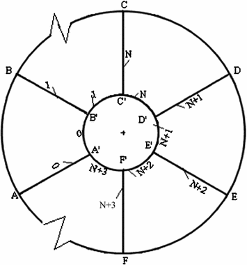

  

  Passive closed recurrent circuit

Let us note that from the methods of investigation of passive asymmetrical recurrent circuits given in this chapter it follows that they are reduced to investigation of symmetrical circuits with account of a number of additional boundary conditions determined by degree of circuit asymmetry.

About the features of differencial and difference equations: currents in passive recurrent circuit (Fig. 6.5a) and in equivalent current—carrying plate (Fig. 6.5b).

Fig. 6.5

Currents in passive recurrent circuit (a), and in equivalent current carrying plate (b)

6.5 Methods of Investigation of Passive Symmetrical Recurrent Circuits Described by “Step” or “Lattice” Functions

6.5.1 Difference Equations, Methods of Their Solution

We proceed to the statement of calculation methods of current distribution in passive recurrent circuits.

Thus, we will accept as initial:

• impedances in longitudinal elements—as per (6.2);

• impedances in cross elements—as per (6.3);

• voltage applied to one or several elements of recurrent circuit.

Let us consider some links (elements) of symmetrical passive recurrent circuit presented in Figs. 6.2, 6.3 or 6.4.

As well as in the previous chapter, let designate serial numbers of cross elements of the circuit as follows: N = 0, 1, 2, …, N − 1, …, N₀₋₁; Let us assign number N to each longitudinal element bounded between two cross elements with numbers N and N + 1. Respectively, the loop bounded between cross elements with numbers N + 1 and N and longitudinal elements with number N will be designated: (N + 1, N). Currents in longitudinal element with number N will be designated as I[N], and in cross element with the same number—J[N]; unknown dependence of these currents on element number N will be designated respectively I _(N) and J _(N).

Further, let us consider a loop formed by cross elements with numbers N + 2, N + 1 and longitudinal elements with number N + 1. For this loop we will write down the equation as per second Kirchhoff’s law [1, 2]:

$$ \left( {{\text{J}}[{\text{N}} + 2] - {\text{J}}[{\text{N}} + 1]} \right){\text{Z}}_{\text{B}} - 2 \cdot {\text{I[N}} + 1]{\text{Z}}_{\text{R}} = 0. $$

(6.5)

According to the first Kirchhoff’s law we have the following relations between these currents:

$$ {\text{J}}[{\text{N}} + 2] = {\text{I}}[{\text{N}} + 2] - {\text{I}}[{\text{N}} + 1];\quad {\text{J[N}} + 1]{\text{I}}[{\text{N}} + 1] - {\text{I}}[{\text{N}} + 0]. $$

(6.6)

After transformation (6.5) taking into account (6.6), we get:

$$ {\text{I}}[{\text{N}} + 2] - (2 + {\sigma )} \cdot {\text{I}}[{\text{N}} + 1] + {\text{I}}[{\text{N}} + 0] = 0. $$

(6.7)

$$ {\text{where}}\,{\text{coefficient}}\quad {\sigma = 2} \cdot \frac{{{\text{Z}}_{\text{R}} }}{{{\text{Z}}_{\text{B}} }} $$

(6.7′)

is determined by the relation of impedance of longitudinal and cross elements of symmetrical recurrent circuit; generally it is a complex number. It is easy to show that this coefficient physically corresponds to the distribution coefficient from the theory of transmission lines [3–6].

Equation (6.7) describes the distribution of currents in all elements of recurrent circuit. It belongs to the class of linear difference equations with constant coefficients [4–7] and has the order equal to two. Equations of this kind correspond to processes described by so-called “step” or “lattice” functions. Features of such a function are, in particular, that its argument changes discretely; respectively, and this function accepts only discrete values [6, 7].

Unlike it—functions describing processes by means of differential equations change continuously, as well as their arguments (except for special discontinuity points not considered here).

In the task class considered, such “step” or “lattice” functions are currents in longitudinal I[N] and in cross elements J[N]; they are connected by the ratio (6.6). Argument of these functions as stated above changes discretely: N = 0, 1,2, …, N − 1,….

Distinction between “step” functions describing processes by means of difference equations, and continuous functions describing processes by means of differential equations has clear physical interpretation. It is necessary for sure to use step functions and methods of their analysis in engineering practice.

Let us consider for example the following two physical problems; for simplicity we select two receivers (Fig. 6.5a, b). In the first example it is necessary to find the distribution of currents in longitudinal and cross elements of passive circuit connected to terminals A, A′ of alternating current source; let us designate the impedance measured between these terminals as Z_EQ.

In the second—it is necessary to find the distribution of current in a conducting plate (for example, copper) connected to terminals AA′ of the same source and with the same impedance between these terminals: ${\text{Z}}_{\text{EQ}} = {\text{idem}}$. Let us note that provided that $\left( {{\text{Z}}_{\text{EQ}} = {\text{idem}}} \right)$ we replace (“equalize”) the circuit with discrete longitudinal and cross impedances of its elements—by conducting plate. Spreading of currents in such a plate (their continuous distribution) is described by Laplace differential equation, and in each point of this plate the Ohm law in differential form ${\Delta } = {\upgamma }\,{\cdot{\text{E}}}$ is true, where $\Delta$—current density in plate element, γ—its specific conductivity, E—electric field intensity. Unlike this continuous distribution of currents in plate, currents in elements of recurrent circuit are distributed discretely according to the solution of corresponding difference equation.

Difference equations can be solved by several methods.

In practice, besides classical [6–8] the method of solution of difference equations by means of Laplace discrete transformation is widely used (Z-transformations). This method [4–7] is similar to that of differential equations solution by means of operational calculation and is especially convenient when solving difference equations or their systems of high order [3].

In the analysis of currents distribution in considered recurrent circuits we will use classical method.

In practical calculations within this method, some modifications of difference equation solution are used as (6.7). Let us consider one of these.

Let us set out the solution of uniform difference Eq. (6.7) in the form:

$$ {\text{I}}_{{({\text{N}})}} = {\text{C}}_{1} \cdot {\text{e}}^{{{\text{k}}_{1} {\text{N}}}} + {\text{C}}_{2} \cdot {\text{e}}^{{{\text{k}}_{2} {\text{N}}}} + \ldots {\text{C}}_{\text{M}} \cdot {\text{e}}^{{{\text{k}}_{\text{M}} {\text{N}}}} $$

(6.8)

Here C₁, C₂,. . ., C_M—constants determined by boundary conditions of problem; k₁, k₂, . . ., k_M—coefficients determined by parameters of recurrent circuit (impedances of its elements).

Therefore, the solution of difference Eq. (6.8) is found if the following are determined:

• constants C₁, C₂,. . ., C_M from boundary conditions depending on peculiarities of recurrent circuit structure;

• coefficients k₁, k₂, . . ., k_M from ratios containing recurrent circuit parameters.

Index M in summation determines the number of summands in (6.8); it corresponds to the order of difference equation and is equal for Eq. (6.7) to two, so M = 1; 2. Let us substitute solution (6.8) to initial Eq. (6.7). After these transformations, we get:

$$ {\text{e}}^{{2{\text{k}}_{\text{M}} }} - (2 + {\sigma )} \cdot {\text{e}}^{{{\text{k}}_{\text{M}} }} + 1 = 0. $$

(6.9)

Equation (6.9) is one of forms of characteristic equation corresponding to difference Eq. (6.7). Let us represent it as:

$$ \left( {{\text{e}}^{{\frac{{{\text{k}}_{\text{M}} }}{2}}} - {\text{e}}^{{ - \frac{{{\text{k}}_{\text{M}} }}{2}}} } \right)^{2} =\upsigma\text{.} $$

From this expression we calculate ${\text{k}}_{\text{M}} \in {\text{k}}_{1} ;{\text{k}}_{2} .$:

$$ {\text{sh}}\frac{{{\text{k}}_{1} }}{2} = + \frac{{\sqrt\upsigma }}{2};\quad {\text{sh}}\frac{{{\text{k}}_{2} }}{2} = - \frac{{\sqrt\upsigma }}{2}. $$

(6.10)

When transforming Eq. (6.9) it is supposed that ${\text{e}}^{{\frac{{{\text{k}}_{\text{M}} }}{2}}} \ne 0$; this condition is always satisfied in the considered class of tasks. Equations (6.10) implicitly determine both coefficients ${\text{k}}_{\text{M}} :{\text{k}}_{1} \,{\text{and}}\,{\text{k}}_{2}$. However, such a type of coefficient representation is inconvenient: inverse hyperbolic functions complicate the type of calculation equation for currents in a closed form. It practically excludes a possibility to use calculation equations in such a form for their joint solution, for example, if they form a system made under both Kirchhoff’s laws or if it is necessary to generalize the analysis results of currents distribution in recurrent circuit.

In some tasks, for example, when designing grounding cables for power transmission line supports [6], when studying the distribution of waves along recurrent circuits modeling processes in high voltage lines it is possible to accept [6]:

$$ {\text{k}}_{1} { \approx } + \sqrt\upsigma ;\quad {\text{k}}_{2} { \approx } - \sqrt\upsigma . $$

Thus, it is supposed that when expanding function ${\text{sh}}\frac{{{\text{k}}_{1} }}{2}$ into a series, only the first term of series is considered. ${\text{sh}}\frac{{{\text{k}}_{1} }}{2}{ \approx }\frac{{{\text{k}}_{1} }}{2}$; similarly, ${\text{sh}}\frac{{{\text{k}}_{2} }}{2}{ \approx }\frac{{{\text{k}}_{2} }}{2}$. However, these approximate expressions are true only for ${\sigma < < 0}\text{.1}$ and for short-circuited rotor windings of A.C. machines usually are not satisfied.

In practice, for the investigation of distribution of currents in elementary conductors (conductor strands) of stator winding [9] or in rotor winding construction elements [13] other modification of solution by any classical method of difference equation as (6.7) has revealed to be more convenient. Its advantage is that it allows obtaining the solution of difference Eq. (6.7) in a closed form. Now we consider it in more detail. Let us perform previously the following additional transformations. Let us designate the value ${\text{e}}^{{{\text{k}}_{\text{M}} }}$ in (6.9) as: ${\text{e}}^{{{\text{k}}_{\text{M}} }} = {\text{a}}_{\text{M}}$, and, as before, for considered class of tasks index M = 1;2. Then Eq. (6.9) takes the form:

$$ {\text{a}}_{\text{M}}^{2} - (2 + {\sigma )} \cdot {\text{a}}_{\text{M}} + 1 = 0. $$

(6.11)

It is also a form of representation of characteristic equation corresponding to difference Eq. (6.7). From its decision we obtain complex values a₁ and a₂ in an explicit form:

$$ {\text{a}}_{1,2} = \frac{{2 +\upsigma \pm \sqrt {\upsigma^{2} + 4\upsigma} }}{2}. $$

(6.12)

Thus, coefficients a₁, a₂ are determined by parameters of recurrent circuit elements.

Let us note that according to Vieta’s theorem [10] the following ratios are true:

$$ {\text{a}}_{1} \cdot {\text{a}}_{2} = 1;\quad {\text{a}}_{1} \cdot {\text{a}}_{2} = 2 +\upsigma\text{.} $$

(6.12′)

These both ratios can be obtained directly using Eq. (6.12) for a₁ and a₂. Ratios (6.12) and (6.12) will be repeatedly used in further calculations.

As a result of transformations (6.11)–(6.12), we obtain the solution of uniform difference Eq. (6.7) in a closed form:

$$ {\text{I}}_{{({\text{N}})}} = {\text{C}}_{1} \cdot {\text{a}}_{1}^{\text{N}} + {\text{C}}_{2} \cdot {\text{a}}_{2}^{\text{N}} , $$

(6.13)

where C₁, C₂—constants determined by boundary conditions; for open and closed recurrent circuits they differ. Let us note that rightness of solution (6.13) can be easily confirmed also directly substituting each of summands into Eq. (6.7), composing Eq. (6.13); number of summands and constants at them (two) are equal thus to the order of difference equation: M = 2.

Equation (6.13) describes the distribution of currents in longitudinal elements of passive recurrent circuit.

Distribution of currents in its cross elements is determined from (6.13) using the first Kirchhoff’s law (6.6):

$$ {\text{J}}_{{({\text{N}})}} = {\text{C}}_{1} \cdot {\text{a}}_{1}^{{{\text{N}} - 1}} \cdot ({\text{a}}_{1} - 1) + {\text{C}}_{2} \cdot {\text{a}}_{2}^{{{\text{N}} - 1}} \cdot ({\text{a}}_{2} - 1). $$

(6.14)

Thus, from the analysis of the obtained Eqs. (6.13) and (6.14) we can draw an important practical conclusion: currents in elements of passive recurrent circuit are distributed under aperiodic law.

We use obtained solution (6.13) of uniform difference Eq. (6.7) in a closed form further for the investigation of currents distribution not only in symmetrical, but also in asymmetrical passive recurrent circuits, as well as in active recurrent circuits of various structure.

Let us note also that results of this analytical investigation of recurrent circuits will also allow us to obtain expressions for MMF of short-circuited rotor windings of A.C. machines (synchronous and induction), to formulate a system of equations for the calculation of modes of these machines, including their operation in nonlinear network.

6.5.2 Pecularities of Currents Distribution in Symmetrical Passive Recurrent Circuits

Let us perform an analysis of some peculiarities of solution (6.13) of difference Eq. (6.7) for currents in relation to the open recurrent circuit. Let us accept for clarity that plus sign in Eq. (6.12) refers to the value of a₁, and minus sign—to value a₂, so |a₂| < |a₁|, herewith, |a₁| > 1, a |a₂| < 1. Let us represent these both complex values as follows:

$$ {\text{a}}_{1} = \text{Re} ({\text{a}}_{1} ) + {\text{j}} \cdot {\text{Im(a}}_{1} ) = \left| {{\text{a}}_{1} } \right| \cdot {\text{e}}^{{{\text{j}}{\upvarphi }_{1} }} ;{\text{a}}_{2} = \text{Re} ({\text{a}}_{2} ) + {\text{j}} \cdot {\text{Im(a}}_{2} ) = \left| {{\text{a}}_{2} } \right| \cdot {\text{e}}^{{{\text{j}}{\upvarphi }_{2} }} . $$

Here, ${\upvarphi }_{1} ,{\upvarphi }_{2}$—phase angles (generally ${\upvarphi }_{1} \ne {\upvarphi }_{2}$).

Then the expression for current (6.13) can be represented as:

$$ {\text{I}}_{{({\text{N}})}} = {\text{C}}_{1} \cdot \left| {{\text{a}}_{1} } \right|^{\text{N}} \cdot {\text{e}}^{{{\text{jN}}{\upvarphi }_{1} }} + {\text{C}}_{2} \cdot \left| {{\text{a}}_{2} } \right|^{\text{N}} \cdot {\text{e}}^{{{\text{jN}}{\upvarphi }_{2} }} . $$

(6.15)

Therefore, in Eq. (6.15), current summands ${\text{I}}_{{({\text{N}})}}$ in different ways change their amplitudes and phases with change of loop number N. For the first current summand ${\text{I}}_{{({\text{N}})}}$ with growth number N the amplitude increases, however, for the second summand with increase of N it decreases; for both current summands ${\text{I}}_{{({\text{N}})}}$ with growth number N, phases also change, however the law of their change is various: it was already noted that ${\upvarphi }_{1} \ne {\upvarphi }_{2}$.

Ratios between constants C₁ and C₂ determine the following possible versions of dependence of longitudinal current ${\text{I}}_{{({\text{N}})}}$ in elements of recurrent circuit on the loop number N:

• with |C₁| ≫|C₂| amplitude of this current with growth number N increases under the exponential law;

• with |C₁| < < |C₂| its amplitude with growth of N is attenuated under the exponential law;

• for other combinations of constants C₁ and C₂ and phase angles ${\upvarphi }_{1} ,{\upvarphi }_{2}$ of both summands, maximum or minimum current amplitude can be reached with growth of N.

6.6 Open Passive Recurrent Circuits. Constants for Calculation of Currents Distribution Calculation Examples

6.6.1 General Comments

It is noted above that constants C₁, C₂ are determined by boundary conditions, and these conditions depend on structural features of recurrent circuit. Previously, however, we can note the following:

• usually in the theory of passive quadripoles it is accepted that voltages U₁, U₂ and currents I₁, I₂ contained in Eq. (6.1) characterize respectively “input (index 1)” and “output (index 2)” of this quadripole; the same refers to recurrent circuits formed by several quadripoles. This condition (existence of “input” and “output”) is generally not obligatory; further, we will consider boundary conditions for the solution of recurrent circuits which have two “input (indices 1 and 2)”; physically it, for example, means that the recurrent circuit is connected to two independent voltage (current) sources of identical frequency differing in both amplitudes and phase angles.

6.6.2 System of Equations for Constants

Let us consider (Fig. 6.2) a passive symmetrical open recurrent circuit consisting of N₀ cross and, respectively, N_0–1 longitudinal elements (N = 0,1,2,… N₀ − 1). Set in values in this circuit are:

• impedances of cross elements Z_B and longitudinal Z_R;

• boundary conditions to determine the constants C₁, C₂ in calculation equations for currents (6.13) and (6.14):

$$ \begin{array}{*{20}c} {{\text{at}}\,{\text{N}} = - 1:{\text{I}}_{( - 1)} = {\text{I}}_{\text{INP}} \cdot {\text{e}}^{{{\text{j}}{\upvarphi }_{\text{INP}} }} ;} \\ {{\text{at}}\,{\text{N}} = {\text{N}}_{0} - 1:{\text{I}}_{{({\text{N}}_{0} - 1)}} = {\text{I}}_{\text{OUT}} \cdot {\text{e}}^{{{\text{j}}{\upvarphi }_{\text{OUT}} }} .} \\ \end{array} $$

(6.16)

Here ${\text{I}}_{\text{INP}} ;{\text{I}}_{\text{OUT}}$—complex amplitudes of currents (phasors), ${\upvarphi }_{\text{INP}} ,{\upvarphi }_{\text{OUT}}$—corresponding phase angles of these currents.

Let us find the distribution of currents in all elements of this recurrent circuit.

Such formulation of boundary conditions is based on the assumption that recurrent circuit is connected from both sides to sources of sinusoidal voltage (Fig. 6.2). Let us turn our attention to two special cases of such a recurrent circuit:

• (a) At phase angles ${\upvarphi }_{\text{INP}} \text{ = 0}^{{^\circ }} ,{\upvarphi }_{\text{OUT}} = \text{0}^{{^\circ }}$ the recurrent circuit has “input” and “output” as currents ${\text{I}}_{( - 1)} \,{\text{and}}\,{\text{I}}_{{({\text{N}}_{0} - 1)}}$ coincident in phase, and their complex amplitudes have the same sign:

  $$ {\text{I}}_{( - 1)} = + {\text{I}}_{\text{INP}} ;{\text{I}}_{{({\text{N}}_{0} - 1)}} = + {\text{I}}_{\text{OUT}} . $$

• (b) At phase angles ${\upvarphi }_{\text{INP}} \text{ = 0}^{{^\circ }} ,{\upvarphi }_{\text{OUT}} = 180^{{^\circ }}$ the recurrent circuit has two “inputs” as currents ${\text{I}}_{( - 1)} \,{\text{and}}\,{\text{I}}_{{({\text{N}}_{0} - 1)}}$ in opposite phase, and their complex amplitudes have opposite signs:

  $$ {\text{I}}_{( - 1)} = + {\text{I}}_{\text{INP}} ;{\text{I}}_{{({\text{N}}_{0} - 1)}} = - {\text{I}}_{\text{OUT}} . $$

Generally, at difference of phase angles

$$ {\upvarphi } = {\upvarphi }_{\text{OUT}} { - \upvarphi }_{{{\text{I}}_{\text{NP}} }} , $$

(6.17)

lying within $0^{{^\circ }} < {\upvarphi < 180}^{{^\circ }}$, the concepts “input” and “output” of recurrent circuit become less distinct; the recurrent circuit can be characterized in these cases also as a circuit with “double-ended power supply”.

Taking into account Eq. (6.17), boundary conditions can be presented in the form:

$$ \begin{array}{*{20}c} {{\text{at}}\quad {\text{N}} = - 1:{\text{I}}_{( - 1)} = {\text{I}}_{\text{NP}} ;} \\ {{\text{at}}\,{\text{N}} = {\text{N}}_{0} - 1:{\text{I}}_{{({\text{N}}_{0} - 1)}} = {\text{I}}_{\text{OUT}} \cdot {\text{e}}^{{{\text{j}}{\upvarphi }}} .} \\ \end{array} $$

(6.16′)

Let us proceed to calculation of constants C₁ and C₂ in Eq. (6.13).

Proceeding from boundary conditions, by means of Eq. (6.13) we get:

$$ {\text{I}}_{( - 1)} = {\text{C}}_{1} \cdot {\text{a}}_{2} + {\text{C}}_{2} \cdot {\text{a}}_{1} ;\quad {\text{I}}_{{({\text{N}}_{0} - 1)}} = {\text{C}}_{1} \cdot {\text{a}}_{1}^{{{\text{N}}_{0} - 1}} + {\text{C}}_{2} \cdot {\text{a}}_{2}^{{{\text{N}}_{0} - 1}} . $$

(6.18)

From the solution of the system of Eq. (6.18) it follows:

$$ {\text{C}}_{1} = \frac{{{\text{I}}_{\text{INP}} \cdot {\text{a}}_{2}^{{{\text{N}}_{0} - 1}} - {\text{I}}_{\text{OUT}} \cdot {\text{e}}^{{{\text{j}}{\upvarphi }}} \cdot {\text{a}}_{1} }}{{{\text{a}}_{2}^{{{\text{N}}_{0} }} - {\text{a}}_{1}^{{{\text{N}}_{0} }} }};\quad {\text{C}}_{2} = \frac{{{\text{I}}_{\text{OUT}} \cdot {\text{e}}^{{{\text{j}}{\upvarphi }}} \cdot {\text{a}}_{2} - {\text{I}}_{\text{INP}} \cdot {\text{a}}_{1}^{{{\text{N}}_{0} - 1}} }}{{{\text{a}}_{2}^{{{\text{N}}_{0} }} - {\text{a}}_{1}^{{{\text{N}}_{0} }} }} $$

(6.19)

Here a₁, a₂ are calculated according to Eq. (6.12), and φ—is determined according to initial data and Eq. (6.17).

6.6.3 Calculation Examples

Example 1

In a passive recurrent circuit with N₀ = 6 cross and, respectively, five longitudinal elements (N = 0, 1, K, 5) the followings are assumed as given:

• impedances of cross elements Z_B = 5 Ohm and longitudinal Z_R = 3 Ohm

• boundary conditions for calculation of currents in the circuit: |I_INP| = |I_OUT| = 100 A.

Let us find the distribution of currents in all elements of this recurrent circuit for two limit values of phase angle difference φ as per (6.17):

$$ {\text{(a)}}\,{\upvarphi = 0}^{{^\circ }} ;{\text{(b}})\,{\upvarphi = 180}^{{^\circ }} . $$

With setting out these two limit values of phase angles φ and values of cross and longitudinal impedances, it is possible to obtain the distribution of currents in the recurrent circuit in extremely clear physical interpretation. Thus, it is possible to simply validate the calculated expressions.

According to the obtained Eqs. (6.13)–(6.19) taking into account values of recurrent circuit parameters we have:

${\text{a}}_{1} = 2.849;{\text{a}}_{2} = 0.351$; respectively, constants of C₁, C₂, are determined as follows:

• (a) at ${\upvarphi = 0}^{{^\circ }} :{\text{C}}_{1} = 0.5318.\quad {\text{C}}_{2} = 35.0345$

• (b) at ${\upvarphi = 180}^{{^\circ }} :{\text{C}}_{1} = - 0.5338.\quad {\text{C}}_{2} = 35.1658.$

Calculation results of currents distribution are given in Tables 6.1 and 6.2.

Table 6.1 Distribution of currents in recurrent circuit elements ${(\upvarphi = 0}^{{^\circ }} )$

Table 6.2 Distribution of currents in recurrent circuit elements ${(\upvarphi = 180}^{{^\circ }} )$

Let us analyze the obtained results.

At ${\upvarphi = 0}^{{^\circ }}$ we have: ${\text{J}}_{(0)} + {\text{J}}_{(1)} + {\text{J}}_{(2)} + {\text{J}}_{(3)} + {\text{J}}_{(4)} + {\text{J}}_{(5)} = {\text{I}}_{{({\text{N}}_{0} - 1)}} - {\text{I}}_{( - 1)} = 0.$

At ${\upvarphi = 180}^{{^\circ }}$ we have: ${\text{J}}_{(0)} + {\text{J}}_{(1)} + {\text{J}}_{(2)} + {\text{J}}_{(3)} + {\text{J}}_{(4)} + {\text{J}}_{(5)} = {\text{I}}_{{({\text{N}}_{0} - 1)}} - {\text{I}}_{( - 1)} = - 200{\text{A}}.$

Thus, both sums of currents in cross elements (at ${\upvarphi = 0}^{{^\circ }} {\text{and}}\,{\upvarphi = 180}^{{^\circ }}$) taking into account boundary conditions satisfy the Kirchhoff’s first law and prove the validity of stated method for passive recurrent circuit calculation.

It should be noted that methods of closed symmetrical recurrent circuits analysis are similar to those of open circuit analysis and differ only in formulation of boundary conditions. They will be considered in the following chapters in relation to active recurrent circuits.

Example 2

In a passive recurrent circuit in Fig. 6.5a with N₀ = 3 (N = 0, 1, 2) cross and, respectively, two longitudinal elements, the followings are assumed as given:

• impedances of cross elements Z_B = 5 Ohm and longitudinal Z_R = 10 Ohm;

• boundary conditions for calculation of currents in circuit: ${\text{I}}_{\text{INP}} = 100{\text{A}}.$

Let us find the distribution of currents in all elements of this recurrent circuit.

According to obtained Eqs. (6.13)–(6.19) taking into account values of recurrent circuit parameters, we have:

a₁ = 5.8284; a₂ = 0.1716; constants of C₁, C₂ are determined as follows: C₁ = 0.0015; C₂ = −1.7158.

Calculation results of currents distribution are given in Table 6.3.

Table 6.3 Distribution of currents in elements of recurrent circuit

It is easy to check the obtained results using both Kirchhoff’s laws [1, 2]. Comparing them with results of solution of two-dimensional Laplace Equation (Fig. 6.5b), we obtain an additional proof of the validity of both solutions: values of currents when the distance increases from voltage source (from terminals AA’) and attenuation that corresponds to physical meaning of task.

6.7 Investigation Methods of Passive Asymmetrical Recurrent Circuits

The methods of analysis of passive asymmetrical circuits developed in this monograph do not depend on their structure and are equally applicable to closed and open circuits including regular.

6.7.1 Difference Equations, Methods of Their Solution

Let us proceed to the statement of calculation methods of currents distribution in asymmetrical recurrent circuits. Thus, we will consider impedances in longitudinal and cross elements.

Let us accept that the impedance Z_Np of one of cross elements with number N_P, for example, element CC’ of asymmetrical recurrent circuit (Fig. 6.2), differs from the impedance of Z_B of other cross elements:

$$ {\text{Z}}_{{{\text{N}}_{\text{P}} }} = {\text{Z}}_{\text{B}} + \Delta {\text{Z}} . $$

(6.20)

The value ∆Z can be generally both positive and negative; in case of circuit break in the element: $\Delta {\text{Z}} \to \infty$. The method also remains true in case of asymmetrically longitudinal impedance of recurrent circuit. If it has several asymmetrical impedances (cross, longitudinal or cross and longitudinal) the method also remains true, and in its realization some modifications are possible; they will be stated in the investigation of calculation features of currents distribution in damper winding elements of synchronous machines and squirrel cages of induction machines.

Let us introduce the following assumption:

• all impedances of recurrent circuit do not depend on currents in its elements, that confirm the recurrent circuit is linear.

Taking into account this assumption, the increment of currents in its elements at the occurrence of asymmetry $(\Delta {\text{Z}} \ne 0 )$ is convenient to present in the form:

$$ {\underline{\underline{\mathbf{I}} } }_{{({\text{N}})}} = {\mathbf{I}}_{{({\text{N}})}} + \Delta {\mathbf{I}}_{{({\text{N)}}}} ;\quad {\underline{\underline{\mathbf{J}} } }_{{({\text{N)}}}} = {\mathbf{J}}_{{({\text{N)}}}} {\mathbf{ + }}\Delta {\mathbf{J}}_{{({\text{N}})}} . $$

(6.21)

Here ${\underline{\underline{\mathbf{I}} } }_{{({\text{N}})}} , {\mathbf{J}}_{{({\text{N}})}}$—resulting currents in circuit elements after the occurrence of asymmetry, $\text{I}_{{({\text{N}})}} ,\text{J}_{{({\text{N)}}}}$—currents in symmetrical circuit (before the occurrence of asymmetry), let us name them as main; let us name increments $\Delta \text{I}_{{({\text{N)}}}} ,\Delta {\text{J}}_{{({\text{N}})}}$ as additional currents. Further it will be shown that in the absence of asymmetry, additional currents are equal to zero;

at $\Delta {\text{Z}} = 0:\Delta \text{I}_{{({\text{N)}}}} = 0\,{\text{and}}\,\Delta {\text{J}}_{{({\text{N}})}} = 0$.

Let us note that in Eq. (6.21) all currents are time complex values (phasors). Let us write down equations under the second Kirchhoff’s law [1, 2] for a number of loops of asymmetrical recurrent circuit; at first, let us allocate in it loops only with symmetrical elements $\left( {{\text{Z}}_{\text{B}} = {\text{idem}}.,{\text{Z}}_{\text{R}} = {\text{idem}}.} \right)$ they satisfy the ratio: $({\text{N}}_{{{\text{P}} + 1}} ,{\text{N}}_{\text{P}} ) < {\text{N}} < ({\text{N}}_{\text{P}} ,{\text{N}}_{{{\text{P}} - 1}} ).$ For these loops, the following is true:

$$ \underline{\underline{\text{J}}}_{{({\text{N)}}}} \cdot {\text{Z}}_{\text{B}} - \underline{\underline{\text{J}}}_{{({\text{N}} - 1 )}} \cdot {\text{Z}}_{\text{B}} - 2 \cdot \underline{\underline{\text{I}}}_{{({\text{N}} - 1)}} \cdot {\text{Z}}_{\text{R}} = 0. $$

With account of (6.20) and (6.21), we have:

$$ {\text{J}}_{{({\text{N}})}} {\text{Z}}_{\text{B}} - {\text{J}}_{{({\text{N}} - 1)}} \cdot {\text{Z}}_{\text{B}} - 2{\text{I}}_{{({\text{N}})}} {\text{Z}}_{\text{R}} + \left[ {\Delta {\text{J}}_{{({\text{N}})}} - \Delta {\text{J}}_{{({\text{N}} - 1)}} } \right]{\text{Z}}_{\text{B}} - 2\Delta {\text{I}}_{{ ( {\text{N}} - 1)}} {\text{Z}}_{\text{R}} = 0. $$

(6.22)

Let us note that in Eq. (6.22) for these loops the first three summands correspond to the distribution of currents in a passive symmetrical circuit; their sum is equal to zero: EMF sources in loop are absent.

This important result allows us to subdivide calculation problem of currents distribution in asymmetrical recurrent circuit into two problems:

• calculation of main currents distribution $\text{I}_{{({\text{N}})}} \,\text{and}\,\text{J}_{{({\text{N)}}}}$ in a symmetrical recurrent circuit before the occurrence of asymmetry in it $\left( {\Delta {\text{Z}} = 0} \right)$;

• calculation of additional currents distribution $\Delta \text{I}_{{({\text{N)}}}} \,{\text{and}}\,\Delta {\text{J}}_{{({\text{N}})}}$ in an asymmetrical recurrent circuit after the occurrence of asymmetry in it $(\Delta {\text{Z}} \ne 0 )$;

resulting currents ${\underline{\underline{\mathbf{I}} } }_{{({\text{N}})}} \,\text{and}\,{\underline{\underline{\mathbf{J}} } }_{{({\text{N)}}}}$ are determined by their addition as per (6.21).

Other summands in (6.22) form the equation:

$$ \left[ {\Delta {\text{J}}_{{({\text{N}})}} - \Delta {\text{J}}_{{({\text{N}} - 1)}} } \right] \cdot {\text{Z}}_{\text{B}} - 2 \cdot \Delta {\text{I}}_{{({\text{N}} - 1)}} \cdot {\text{Z}}_{\text{R}} = 0. $$

(6.23)

Relation between additional currents $\Delta {\text{J}}\,{\text{and}}\,\Delta {\text{I}}$ is determined by the first Kirchhoff’s law similarly to Eq. (6.6):

$$ \Delta {\text{J[N]}} = \Delta {\text{I[N]}} - \Delta {\text{I[N}} - 1 ];\Delta {\text{J[N}} - 1 ]= \Delta {\text{I[N}} - 1] - \Delta {\text{I[N}} - 2]. $$

(6.6′)

As a result, we obtain the following difference equation of the second order:

$$ \Delta {\text{I[N}} + 2] - (2 +\upsigma) \cdot \Delta {\text{I[N}} + 1 ]+ \Delta {\text{I[N}} + 0 ]= 0 $$

(6.7″)

It is similar to Eq. (6.7), but describes the distribution of additional currents caused by asymmetry in recurrent circuit. The solution of this difference equation after transformations has the form:

for circuit elements with numbers N < N_P:

$$ \Delta {\text{I}}_{{({\text{N}})}} = {\text{C}}_{1} \cdot {\text{a}}_{1}^{\text{N}} + {\text{C}}_{2} \cdot {\text{a}}_{2}^{\text{N}} , $$

(6.24)

for circuit elements with numbers $\text{N} \ge \text{N}_{\text{P}}$:

$$ \Delta {\text{I}}_{{({\text{N}})}} = {\text{C}}_{3} \cdot {\text{a}}_{1}^{\text{N}} + {\text{C}}_{4} \cdot {\text{a}}_{2}^{\text{N}} . $$

(6.25)

Here C₁, C₂, C₃, C₄—constants determined by boundary conditions for additional currents of recurrent circuit; therefore, they depend on its structure and damage rate of its elements (asymmetry degree). Coefficients a₁, a₂ are determined by parameters of recurrent circuit elements before damage and do not depend on the asymmetry degree; they are found according to Eq. (6.12).

Equations (6.24) and (6.25) correspond to the distribution of additional currents in longitudinal elements. Equations for additional currents in cross elements:

for circuit elements with numbers N < N_P:

$$ \Delta {\text{J}}_{{({\text{N}})}} = {\text{C}}_{1} \cdot {\text{a}}_{1}^{{{\text{N}} - 1}} \cdot ({\text{a}}_{1} - 1) + {\text{C}}_{2} \cdot {\text{a}}_{2}^{{{\text{N}} - 1}} \cdot ({\text{a}}_{2} - 1), $$

(6.26)

for circuit elements with numbers N > N_P:

$$ \Delta {\text{J}}_{{({\text{N}})}} = {\text{C}}_{3} \cdot {\text{a}}_{1}^{{{\text{N}} - 1}} \cdot ({\text{a}}_{1} - 1) + {\text{C}}_{4} \cdot {\text{a}}_{2}^{{{\text{N}} - 1}} \cdot ({\text{a}}_{2} - 1), $$

(6.27)

for circuit elements with numbers N = N_P:

$$ \Delta {\text{J}}_{{({\text{N}})}} = {\text{C}}_{3} \cdot {\text{a}}_{1}^{{{\text{N}}_{\text{P}} }} - {\text{C}}_{1} \cdot {\text{a}}_{1}^{{{\text{N}}_{\text{P}} - 1}} + {\text{C}}_{4} \cdot {\text{a}}_{1}^{{{\text{N}}_{\text{P}} }} - {\text{C}}_{2} \cdot {\text{a}}_{2}^{{{\text{N}}_{\text{P}} - 1}} . $$

(6.28)

6.7.2 Constants of Asymmetrical Passive Open Recurrent Circuit; Their Determination

6.7.2.1 General Case of Asymmetry: ${\mathbf{0}} < {\varvec{\Delta}}{\mathbf{\rm Z}} < \infty$

Let us allocate in recurrent circuit loops containing asymmetrical cross elements with number Np; its impedance corresponds to Eq. (6.20).

In order to determine the constants C₁, C₂, C₃, C₄ from boundary conditions and expressions for calculation of additional currents in the circuit, let us use the following four equations:

• (a) It is easy to obtain two equations under the second Kirchhoff’s law for two loops containing asymmetrical element with number N_P;

for circuit loop with number (N_P, N_P − 1):

$$ {\text{J}}_{{({\text{N}}_{\text{P}} )}} {\text{Z}}_{\text{B}} - {\text{J}}_{{({\text{N}}_{\text{P}} - 1)}} {\text{Z}}_{\text{B}} - 2{\text{I}}_{{({\text{N}}_{\text{P}} - 1)}} {\text{Z}}_{\text{R}} + \Delta {\text{J}}_{{({\text{N}}_{\text{P}} )}} {\text{Z}}_{{{\text{N}}_{\text{P}} }} - \Delta {\text{J}}_{{({\text{N}}_{\text{P}} - 1)}} {\text{Z}}_{\text{B}} - 2\Delta {\text{I}}_{{({\text{N}}_{\text{P}} )}} {\text{Z}}_{\text{R}} + {\text{J}}_{{({\text{N}}_{\text{P}} )}} \Delta {\text{Z}} = 0; $$

(6.29)

for circuit loop with number (N_P+1, N_P):

$$ {\text{J}}_{{({\text{N}}_{\text{P}} + 1)}} {\text{Z}}_{\text{B}} - {\text{J}}_{{({\text{N}}_{\text{P}} )}} {\text{Z}}_{\text{B}} - 2{\text{I}}_{{({\text{N}}_{\text{P}} )}} {\text{Z}}_{\text{R}} + \Delta {\text{J}}_{{({\text{N}}_{\text{P}} + 1)}} {\text{Z}}_{\text{B}} -\Delta {\text{J}}_{{({\text{N}}_{\text{P}} )}} {\text{Z}}_{{{\text{N}}_{\text{P}} }} - 2\Delta {\text{I}}_{{({\text{N}}_{\text{P}} )}} {\text{Z}}_{\text{R}} -{\text{J}}_{{({\text{N}}_{\text{P}} )}} \Delta {\text{Z}} = 0. $$

(6.30)

After transformation of these equations, we get:

$$ \Delta {\text{I}}_{{({\text{N}}_{\text{P}} )}} \left( {1 + \frac{{\Delta {\text{Z}}}}{{{\text{Z}}_{\text{B}} }}} \right) - \Delta {\text{I}}_{{({\text{N}}_{\text{P}} - 1)}} \left( {2 +\upsigma + \frac{{\Delta {\text{Z}}}}{{{\text{Z}}_{\text{B}} }}} \right) + {\text{I}}_{{({\text{N}}_{\text{P}} - 1)}}= - {\text{J}}_{{({\text{N}}_{\text{P}} )}} \frac{{\Delta {\text{Z}}}}{{{\text{Z}}_{\text{B}} }}; $$

(6.31)

$$ \Delta {\text{I}}_{{({\text{N}}_{\text{P}} + 1)}} - \Delta {\text{I}}_{{({\text{N}}_{\text{P}} )}} \left( {2 +\upsigma + \frac{{\Delta {\text{Z}}}}{{{\text{Z}}_{\text{B}} }}} \right) + {\text{I}}_{{({\text{N}}_{\text{P}} - 1)}} \left( {1 + \frac{{\Delta {\text{Z}}}}{{{\text{Z}}_{\text{B}} }}} \right) = {\text{J}}_{{({\text{N}}_{\text{P}} )}} \frac{{\Delta {\text{Z}}}}{{{\text{Z}}_{\text{B}} }}; $$

(6.32)

• (b) Two other equations result from the recurrent circuit structure. For closed and open recurrent circuits they are different.

Let us consider the determination of constants for an open circuit containing N₀ cross elements. For such a circuit the following two equations under the first Kirchhoff’s law are true:

$$ \begin{array}{*{20}c} {\Delta {\text{I}}_{(0)} = \Delta {\text{J}}_{(0)} ;\Delta {\text{I}}_{{({\text{N}}_{0} - 2)}} = - \Delta {\text{J}}_{{({\text{N}}_{0} - 1)}} \,{\text{or}}} \\ {{\text{C}}_{1} \cdot {\text{a}}_{2} + {\text{C}}_{2} \cdot {\text{a}}_{1} = 0.\quad {\text{C}}_{3} \cdot {\text{a}}_{1}^{{{\text{N}}_{0} - 1}} + {\text{C}}_{4} \cdot {\text{a}}_{2}^{{{\text{N}}_{ 0} - 1}} = 0.} \\ \end{array} $$

(6.33)

To obtain calculation expressions for additional currents in elements of open recurrent circuit, it is necessary to determine constants C₁, C₂, C₃, C₄.

Equations (6.31)–(6.33) form a system for their determination.

After transformation of these equations, the system takes the form:

$$ \begin{array}{*{20}c} {{\text{M}} \cdot {\text{C}}_{1} + {\text{T}} \cdot {\text{C}}_{2} + {\text{A}} \cdot {\text{C}}_{3} + {\text{B}} \cdot {\text{C}}_{4} = - {\text{J}}_{{({\text{N}}_{\text{P}} )}} \frac{{\Delta {\text{Z}}}}{{{\text{Z}}_{\text{B}} }};} \\ {({\text{M}} + {\text{H}}) \cdot {\text{C}}_{1} + ({\text{T}} + {\text{K)}} \cdot {\text{C}}_{2} + ({\text{A}} + {\text{F)}} \cdot {\text{C}}_{3} + ({\text{B}} + {\text{S}}) \cdot {\text{C}}_{4} = 0;} \\ {{\text{N}} \cdot {\text{C}}_{1} + {\text{P}} \cdot {\text{C}}_{2} = 0;\quad {\text{Q}} \cdot {\text{C}}_{3} + {\text{R}} \cdot {\text{C}}_{4} = 0.} \\ \end{array} $$

(6.34)

Values of system coefficients are given in Appendix 6.1.

The order of this system (r = 4) does not depend on the number of links of recurrent circuit being the advantage of method in practical calculations.

From this system we obtain constants for calculation of algebraic adjuncts for currents:

$$ {\text{C}}_{\text{i}} = {\text{J}}_{{({\text{N}}_{\text{P}} )}} \cdot \frac{{\Delta {\text{Z}}}}{{{\text{Z}}_{\text{B}} }} \cdot \frac{{{\text{D}}_{\text{i}} }}{{{\text{D}}_{\text{S}} }}. $$

Here D_S—system determinant, D_i—corresponding algebraic adjuncts; i = 1, 2, 3, 4.

System determinant (N_B = N₀₋₂):

$$ \begin{aligned} {\text{D}}_{\text{S}} & = {\text{a}}_{1}^{{{\text{N}}_{\text{B}} + 1}} \left( {{\text{a}}_{1}^{2} - 1 + 2{\text{a}}_{1} \frac{{\Delta {\text{Z}}}}{{{\text{Z}}_{\text{B}} }} - 2\frac{{\Delta {\text{Z}}}}{{{\text{Z}}_{\text{B}} }}} \right) + {\text{a}}_{2}^{{{\text{N}}_{\text{B}} + 1}} \left( {{\text{a}}_{2}^{2} - 1 + 2{\text{a}}_{2} \frac{{\Delta {\text{Z}}}}{{{\text{Z}}_{\text{B}} }} - 2\frac{{\Delta {\text{Z}}}}{{{\text{Z}}_{\text{B}} }}} \right) \\ & \quad + \frac{{\Delta {\text{Z}}}}{{{\text{Z}}_{\text{B}} }}\left( {{\text{a}}_{1}^{{ 2 {\text{N}}_{\text{P}} - {\text{N}}_{\text{B}} - 1}} + {\text{a}}_{2}^{{ 2 {\text{N}}_{\text{P}} - {\text{N}}_{\text{B}} - 1}} } \right)(2 - {\text{a}}_{1} - {\text{a}}_{2} ). \\ \end{aligned} $$

(6.35)

Let us note that the third multiplier in the last summand, in brackets, according to Vieta theorem (6.12) equals: $2 - {\text{a}}_{1} - {\text{a}}_{2} = - 2\frac{{{\text{Z}}_{\text{R}} }}{{{\text{Z}}_{\text{B}} .}}$

Algebraic adjuncts of system:

$$ \begin{array}{*{20}l} {{\text{D}}_{1} = \left( {{\text{a}}_{1}^{{{\text{N}}_{\text{B}} - {\text{N}}_{\text{P}} - 1}} + {\text{a}}_{1}^{{{\text{N}}_{\text{B}} - {\text{N}}_{\text{P}} + 2}} } \right)\left( {{\text{a}}_{1} - 1} \right),\quad {\text{D}}_{2} = \left( {{\text{a}}_{1}^{{{\text{N}}_{\text{B}} - {\text{N}}_{\text{P}} }} + {\text{a}}_{1}^{{{\text{N}}_{\text{P}} - {\text{N}} - 3}} } \right)\left( {1 - {\text{a}}_{1} } \right),} \hfill \\ {{\text{D}}_{3} = \left( {{\text{a}}_{1}^{{{\text{N}}_{\text{P}} - {\text{N}}_{\text{B}} - 1}} + {\text{a}}_{1}^{{ - {\text{N}}_{\text{B}} - {\text{N}}_{\text{P}} - 2}} } \right)\left( {{\text{a}}_{1} - 1} \right),\quad {\text{D}}_{4} = \left( {{\text{a}}_{1}^{{{\text{N}}_{\text{P}} + {\text{N}}_{\text{B}} + 1}} + {\text{a}}_{1}^{{{\text{N}}_{\text{B}} - {\text{N}}_{\text{P}} }} } \right)\left( {1 - {\text{a}}_{1} } \right).} \hfill \\ \end{array} $$

(6.36)

We obtained that the system determinant D_S linearly depends on the asymmetry ∆Z of recurrent circuit, and additions D₁, D₂, D₃, D₄ do not depend on ∆Z.

The obtained calculation Eqs. (6.35) and (6.36) prove that in a symmetrical recurrent circuit (at ∆Z = 0) the additional currents in its elements are absent. It proves the validity of developed calculation method of asymmetrical open recurrent circuits.

6.7.2.2 Asymmetry Limit Case: Circuit Break (∆Z → ∞)

Checking results

Calculation expressions for currents in asymmetrical recurrent circuits in relation to short-circuited rotor loops are obtained for the first time [13], and, therefore, they require additional checks.

Let us consider one of them: at ∆Z → ∞ the resulting current in element with number N = N_p should be obtained from equations equal to zero.

At circuit break in the element (∆Z → ∞) the calculation expression for currents follows from the obtained expressions by passage to the limit [8–10]. As a result, we have:

$$ {\text{C}}_{\text{i}} = {\text{J}}_{{ ( {\text{N}}_{\text{P}} )}} \cdot \frac{{{\text{D}}_{\text{i}} }}{{{\text{D}}_{\infty } }}{\text{for}}\,{\text{i}} = 1,2,3,4. $$

(6.37)

Here, D_i—as per (6.36) for i = 1, 2, 3, 4.

$$ \begin{aligned} {\text{D}}_{\infty } & = 2{\text{a}}_{1}^{{{\text{N}}_{\text{B}} + 1}} ({\text{a}}_{1} - 1) + 2{\text{a}}_{2}^{{{\text{N}}_{\text{B}} + 1}} ({\text{a}}_{2} - 1) \\ & \quad + \left( {{\text{a}}_{1}^{{ 2 {\text{N}}_{\text{P}} -{\text{N}}_{\text{B}} - 1}} + {\text{a}}_{2}^{{ 2 {\text{N}}_{\text{P}} -{\text{N}}_{\text{B}} - 1}} } \right)(2 - {\text{a}}_{ 1} -{\text{a}}_{ 2} ). \\ \end{aligned} $$

(6.38)

It follows from this equation that at N = N_P and ∆Z → ∞ the absolute value of additional current in cross element is equal to the main one, but opposite in sign $\Delta {\text{J}}_{{ ( {\text{N}}_{\text{P}} )}} = - {\text{J}}_{{ ( {\text{N}}_{\text{P}} ),}} ,$ so the resulting current $\underline{\underline{\text{J}}}_{{ ( {\text{N}}_{\text{P}} )}}$ in the element with this number is equal to zero as per (6.21). This result is an additional proof of the method developed.

It should be noted that analysis methods of closed asymmetrical recurrent circuits are similar to those of open circuits and differ only in formulation of boundary conditions. They will be considered in the following chapters in relation to active recurrent circuits.

6.7.3 Calculation Examples

Let us continue the consideration of examples given in the previous paragraph for angle ${\upvarphi } = 180{^\circ }$. Distribution of currents in symmetrical recurrent circuit for this case is given in Table 6.2.

6.7.3.1 Asymmetry $\Delta {\mathbf{Z}}_{{{\mathbf{N}}_{{\mathbf{P}}} }} = 2$

Let us accept in addition that in cross elements with number ${\text{N}} = {\text{N}}_{\text{P}} = 2$ of this circuit there is an asymmetry: $\Delta {\text{Z}} = 2$; circuit asymmetry degree $\frac{{\Delta {\text{Z}}}}{{{\text{Z}}_{\text{B}} }} = 0.4$. Then we find the distribution of currents in this asymmetrical circuit.

System determinant according to Eq. (6.35) is equal to: ${\text{D}}_{\text{S}} = 1611.749$; algebraic adjuncts according to Eq. (6.36) are equal to: ${\text{D}}_{1} = 121.896;{\text{D}}_{ 2} = - 15.018;{\text{D}}_{ 3} = 0.0804;{\text{D}}_{ 4} = - 2831.989.$

Calculation results of distribution of additional currents in recurrent circuit elements are given in Table 6.4

Table 6.4 Distribution of additional currents $\left( {{\upvarphi = 180}^{{^\circ }} } \right)$

Calculation results of resulting currents distribution in recurrent circuit elements are given in Table 6.5.

Table 6.5 Distribution of resulting currents in recurrent circuit elements $\left( {{\upvarphi = 180}^{{^\circ}}} \right)$

From calculation results, it follows:

• at asymmetry $\left( {\Delta {\text{Z}} = 2;\quad \frac{{\Delta {\text{Z}}}}{\text{ZB}} = 0.4} \right)$ in comparison with the symmetrical recurrent circuit (Table 6.2), the cross element with number ${\text{N}} = {\text{N}}_{\text{P}} = 2$ is unloaded, however, the currents passing through adjacent cross elements increase, and the extent of distortion decreases with an increase in the distance from asymmetrical element;

• the sum of currents in cross elements satisfies the first Kirchhoff’s law and proves validity of developed calculation method for asymmetrical passive recurrent circuits:

$$ \underline{\underline{\text{J}}}_{(0)} + \underline{\underline{\text{J}}}_{(1)} + \underline{\underline{\text{J}}}_{(2)} + \underline{\underline{\text{J}}}_{(3)} + \underline{\underline{\text{J}}}_{(4)} + \underline{\underline{\text{J}}}_{(5)} = \underline{\underline{\text{I}}}_{{({\text{N}}_{ 0} - 1)}} - \underline{\underline{\text{I}}}_{( - 1)} = - 200({\text{A}}). $$

6.7.3.2 Limiting Case

Limit case: circuit break $(\Delta {\text{Z}} \to \infty )$ in cross element with number ${\text{N}} = {\text{N}}_{\text{P}} = 2$.

Checking results.

According to Eqs. (6.37) and (6.38) we have:

D_S = 690.269; constants are equal to C₁ = −1.9112; C₂ = 0.2354; ${\text{C}}_{ 3} = - 1.2605 \cdot 10^{ - 3} ;{\text{C}}_{ 4} = 44.4014.$

The additional current in the element with number ${\text{N}} = {\text{N}}_{\text{P}} = 2\,(\Delta {\text{Z}} \to \infty )$ is equal to: ∆J_(N) = 10.82; resulting current according to Table 6.2 is equal to: $\underline{\underline{\text{J}}}_{{ ( {\text{N)}}}} = 0$. This result also proves the validity of developed calculation method.

6.8 Appendix 6.1

System coefficients to determine the constants C₁, C₂, C₃, C₄.

$$ {\text{M}} = - {\text{a}}_{1}^{{{\text{N}}_{\text{P}} - 1}} \left( {{\text{a}}_{1} + \frac{{\Delta {\text{Z}}}}{{{\text{Z}}_{\text{B}} }}} \right);\quad {\text{A}} = {\text{a}}_{1}^{{{\text{N}}_{\text{P}} }} \left( {1 + \frac{{\Delta {\text{Z}}}}{{{\text{Z}}_{\text{B}} }}} \right);\quad {\text{H}} = {\text{a}}_{1}^{{{\text{N}}_{\text{P}} - 1}} \left( {1 + \frac{{\Delta {\text{Z}}}}{{{\text{Z}}_{\text{B}} }}} \right); $$

$$ {\text{F}} = - {\text{a}}_{1}^{{{\text{N}}_{\text{P}} }} \left( {{\text{a}}_{ 2} { + }\frac{{\Delta {\text{Z}}}}{{{\text{Z}}_{\text{B}} }}} \right) ;\quad {\text{N}} = {\text{a}}_{ 2} ;\quad {\text{Q}} = {\text{a}}_{1}^{{{\text{N}}_{\text{B}} + 1}} . $$

Coefficients T, B, K, S, P, R can be obtained respectively from those M, A, H, F, N, Q by replacement a₁ by a₂ and, respectively, a₂ by a₁.

List of Symbols

A, B, C, D:

Constants determined by quadripole impedances;

C₁, C₂, …, C_M :

Constants for calculation of currents determined by boundary conditions of recurrent circuit;

I[N], J[N]:

Currents in longitudinal and cross element of recurrent circuit with number N by solution of difference equations;

${\text{I}}_{{({\text{N}})}} \,{\text{and}}\,{\text{J}}_{{({\text{N}})}}$ :

Dependence of currents in recurrent circuit elements on element number N;

${\text{I}}_{\text{INP}} ,{\text{I}}_{\text{OUT}}$ :

Complex amplitudes of currents at recurrent circuit input and output;

$\Delta \text{I}_{{({\text{N)}}}} ,\Delta {\text{J}}_{{({\text{N}})}}$ :

Additional currents in longitudinal and cross elements of asymmetrical recurrent circuit;

k₁, k₂, …, k_M :

Coefficients determined by impedances of recurrent circuit elements;

N:

Element number of recurrent circuit;

N₀ :

Number of elements in recurrent circuit;

N_P :

Asymmetrical element number;

U₂, I₁ :

Voltage and current at passive quadripole input;

U₂, I₂ :

Voltage and current at passive quadripole output;

${\text{Z}}_{{{\text{B}}_{1} }} ,{\text{Z}}_{{{\text{B}}_{3} }} ,{\text{Z}}_{{{\text{R}}_{1} }} ,{\text{Z}}_{{{\text{R}}_{3} }}$ :

Impedances of recurrent circuit elements;

Z_NP :

Impedance of asymmetrical element;

∆Z:

Additional impedance of asymmetrical element;

σ:

Relation determined by impedances of elements of symmetrical recurrent circuit;

${\upvarphi }_{\text{INP}} ,{\upvarphi }_{\text{OUT}}$ :

Phase angles of currents at recurrent circuit input and output

6.9 Brief Conclusions

• 1. In passive symmetrical recurrent circuits (∆Z = 0) equations for calculation of currents distribution in elements contain two components; both vary depending on the element number (N) under the aperiodic law.

• 2. In passive asymmetrical recurrent circuits (∆Z ≠ 0) calculation of currents distribution in elements can be reduced to the solution of two problems:

  • calculation of distribution of the main currents in elements of symmetrical recurrent circuits (∆Z = 0);

  • calculation of distribution of additional currents which depends on the distribution of the main;

  • calculation of distribution of resulting currents is reduced to the summation of the main and additional currents for the same elements.

• 3. Equations for calculation of distribution of additional currents contain two components in elements of an asymmetrical recurrent circuit; both vary depending on the element number (N) under the aperiodic law.

• 4. For limiting case—cross element break (∆Z → ∞)—the main and additional currents are equal in amplitude and are opposite in phase so the resulting current is equal to zero. It proves validity of the obtained equations. 

• 5. Numerical examples also prove validity of the obtained calculation expressions.

References

I. Monographs, general courses, textbooks
Demirchyan K.S., Neyman L.R., Korovkin N.V., Theoretical Electrical Engineering Moscow, St. Petersburg: Piter, Vol. 1, 2, 2009. (In Russian).
Kuepfmueller K., Kohn G., Theoretische Elektrotechnik und Elektronik. 15 Aufl. Berlin, N. Y.: Springer. 2000. (In German).
Carson J.R., Elektrische Ausgleichvorgaenge und Operatorenrchnung. Berlin: Springer, 1929. (In German).
Doetsch G., Handbuch der Laplace – Transformation. Baende 1,2,3. Basel: Verlag Birkhaeuser, 1973. (In German).
Doetsch G., Einfuehrung in Theorie und Anwendung der Laplace – Transformation. Basel: Verlag Birkhaeuser, 1976. (In German).
Ruedenberg R., Elektrische Schaltvorgaenge. Berlin, Heidelberg, N.-Y.: Springer, 1974. (In German).
Gardner M., Barnes J., Transients in Linear Systems Studied by the Laplace Transformation, N. Y.: J. Wiley, 1942.
Jeffris H., Swirles B., Methods of Mathematical Physics. Third Edition, Vol. 1 – Vol. 3, Cambridge: Cambridge Univ. Press, 1966.
Boguslawsky I.Z., A.C. motors and generators. The theory and investigation methods by their operation in networks with non linear elements. Monograph. TU St. Petersburg Edit., 2006. Vol. 1; Vol.2. (In Russian).
Korn G., Korn T., Mathematical Handbook, N. Y.: McGraw – Hill, 1961.
II. Asynchronous machines. Papers, inventor’s certificates, patents
Boguslawsky I.Z., Methods of MMF investigation for the cage rotor damaged bars. Proc.: The problems of development and operation of new types of power equipment. Department of electrical power problems in Russian Academy of Science. St. Petersburg. 2003. (In Russian.).
Boguslawsky I.Z., Demirtschian K.S., Stationaere Stromverteilung in unregelmaessigen und unsymmetrischen kurzgeschlossenen Laeuferwicklungen von Wechselstrommaschinen. Archiv fuer Elektrotechnik, 1992, № 6 (In German).
III. Synchronous machines. Papers, inventor’s certificates, patents
Demirchyan K.S., Boguslawsky I.Z., Current flowing in damper winding bars of different resistivity in a heavy- duty low speed motor. Proceedings of the Russian Academy of Sciences. Energetika i Transport, 1980, #2. (In Russian).
Boguslawsky I.Z., Currents and harmonics MMFs in a damper winding with damaged bar at a pole. Power Eng. (New York), 1985, #1.
Author information
Authors and Affiliations
Corresponding author
Rights and permissions
Copyright information
© 2017 Springer Japan KK
About this chapter
Cite this chapter
Boguslawsky, I., Korovkin, N., Hayakawa, M. (2017). Passive Quadripoles; Recurrent Circuits of Various Structure: Investigation of Their Peculiarities for Modeling Process of Currents Distribution in Short-Circuited Rotor Windings. In: Large A.C. Machines. Springer, Tokyo. https://doi.org/10.1007/978-4-431-56475-1_6
Download citation
DOI: https://doi.org/10.1007/978-4-431-56475-1_6
Published:
Publisher Name: Springer, Tokyo
Print ISBN: 978-4-431-56473-7
Online ISBN: 978-4-431-56475-1
eBook Packages: EngineeringEngineering (R0)