Inverse Problems for Trees

Abstract

This chapter is devoted to the solution of the inverse problem for Schrödinger operators on metric trees.

This chapter is devoted to the solution of the inverse problem for Schrödinger operators on metric trees. The problem has been studied in [68, 69, 73, 109, 509, 510] (see also later references by the authors). We follow the approach developed in [37, 44] based on BC-method for the one-dimensional Schrödinger equation.

For trees it is customary to consider as the contact set the set of all degree one vertices

$$\displaystyle \begin{aligned} \left\{ V^m : \deg V^m = 1 \right\} \end{aligned} $$

(20.1)

—the graph’s boundary. The magnetic potential on any metric tree can be eliminated, hence the set of spectral data will consist of the two equivalent sets:

• the M-function ${\mathbf {M}}(\lambda ) = {\mathbf {M}}_{{\mathbf {T}}} (\lambda )$,

  or

• the dynamical response operator ${\mathbf {R}}^T$, known for sufficiently large $T$.

The inverse problem for trees can be solved by a leaf-pealing procedure where the metric tree, potential, and vertex conditions are recovered step by step starting from a region situated close to the boundary (Fig. 20.1). In this way the inverse problem is reduced to the inverse problem on a smaller tree. The whole operator is reconstructed step-by-step.

Fig. 20.1

A metric tree

By using the two different sets of spectral data (the M-function and the dynamical response operator) we are going to make our presentation more transparent and avoid difficulties which appear if just one set is used. For example the dynamical response operator is more suitable for the reconstruction of the potential on the pendant edges having as one of the endpoints a degree one contact vertex, while the reduction to a smaller tree is easier if the Titchmarsh-Weyl M-functions are used.

20.1 Obvious Ambiguities and Limitations

Before solving the inverse problem let us discuss necessary assumptions and possible ambiguities.

Observation 20.1

The magnetic potential in the Schrödinger equation on a tree can be removed, leading to a certain similarity transformation of the M-function. Let us choose any point $x_0 \in {\mathbf {T}}$ and consider the unitary transformation of multiplication by the function (generalising (4.10))

$$\displaystyle \begin{aligned} \exp \left( i \int_{x_0}^x a(y) dy \right) , \end{aligned}$$

where $a$ is the magnetic potential and the integration is taken along the shortest path connecting $x_0$ and $x.$¹ Then the operators $L_{q,a}$ and $L_q$ are connected by

$$\displaystyle \begin{aligned} e^{ - i \int_{x_0}^x a(y) dy} L_{q,a} e^{ i \int_{x_0}^x a(y) dy} = L_{q}.\end{aligned}$$

Introducing the diagonal $M_\partial \times M_\partial = (N+1) \times (N+1)$ matrix

$$\displaystyle \begin{aligned} {\mathbf{U}} _{x_j,x_j} = e^{ i \int_{x_0}^{x_j} a(y) dy}, \quad x_j \in \partial {\mathbf{T}}, \end{aligned} $$

(20.2)

we get an explicit relation connecting the corresponding M-functions

$$\displaystyle \begin{aligned} {\mathbf{M}}_{L_{q,a}} ( \lambda) = {\mathbf{U}} {\mathbf{M}}_{L_q} (\lambda) {\mathbf{U}}^{-1}. \end{aligned} $$

(20.3)

It follows that it is impossible to reconstruct the exact form of the magnetic potential—only the integrals $\displaystyle \int _{x_i}^{x_j} a(y) dy$ between the contact points. Having this in mind we restrict our consideration in this chapter to Schrödinger operators with zero magnetic potential.

Physicists use to say that there is no magnetic field in one dimension.

Observation 20.2

Let $L_q^S$ be a Schrödinger operator on a metric graph ${\mathbf {T}}.$ Let $\theta (x)$ be a real-valued function on ${\mathbf {T}}$, constant on every edge $E_n$ and equal to zero on all pendant edges:

$$\displaystyle \begin{aligned} \theta (x) = \left\{ \begin{array}{lll} \theta_n, & x \in E_n, & E_n\mbox{ is not a pendant edge}; \\ 0, & x \in E_n, & E_n\mbox{ is a pendant edge}. \end{array} \right.\end{aligned}$$

Then the similarity transformation

$$\displaystyle \begin{aligned} {} L_q^{{\mathbf{S}}} \; \; \rightarrow \; \; L_q^{\hat{{\mathbf{S}}}} (\theta) = e^{-i \theta (x)} L_q^S e^{i \theta (x)} \end{aligned} $$

(20.4)

preserves the M-function. In other words, the operators $L_q^{\hat {{\mathbf {S}}}}$ and $L_q^{{\mathbf {S}}} (\theta )$ have precisely the same Titchmarsh-Weyl matrices, but the vertex conditions at internal vertices in may be different, since they are described by the scattering matrices ${\mathbf {S}}$ and $\hat {{\mathbf {S}}}.$ The relation between these matrices is rather explicit, but we leave the exact form of the relation as a problem for the readers.

Problem 89

Determine the formula that describes the relation between the matrices ${\mathbf {S}}$ and $\hat {{\mathbf {S}}}$, explaining how the vertex conditions are changed under the similarity transformation (20.4).

It follows that the inverse problem can be solved only up to the similarity transformation (20.4). Note that this transformation does not change the metric graph ${\mathbf {T}}$ and the potential $q$, but does affect the vertex conditions.

Observation 20.3

If the matrix parametrising the vertex conditions has zero entries, then it might happen that the metric graph cannot be reconstructed uniquely. Such a counterexample was first presented in [335], where the Laplace operator $L^{\mathbf {S}}$ on the cross graph depicted at Fig. 20.2 was considered. If the vertex scattering matrix $S^1$ associated with the central vertex $V^1 = \{ x_2, x_4, x_6, x_8 \}$ is chosen such that there is no transition between the opposite branches of the cross and no reflection from the central vertex, then all crosses with equal distances between the neighbouring pendant vertices $d(x_{1} ,x_{3}), \; d(x_3,x_5), \; d(x_5,x_7), \; d(x_7,x_1)$ may have identical M-functions.

Fig. 20.2

Metric cross. First published in Proc. AMS in 140 (2012), published by the American Mathematical Society. Ⓒ 2012 by the American Mathematical Society

The matrix $S^1$ possessing the described properties and being scaling invariant has the form

$$\displaystyle \begin{aligned} S^1 = \left( \begin{array}{cccc} 0 & \alpha & 0 & \beta \\ \alpha & 0 & \beta & 0 \\ 0 & \beta & 0 & - \alpha \\ \beta & 0 & - \alpha & 0 \end{array} \right) , \; \; \; \alpha^2 + \beta^2 = 1, \; \; \alpha, \beta \in \mathbb (-1,1). \end{aligned}$$

The corresponding M-function is calculated in Appendix 1:

$$\displaystyle \begin{aligned} {} \begin{array}{l} {\mathbf{M}}(\lambda) = \\ -k \left( \begin{array}{cccc} \frac{ \alpha^2 c_{1-3} s_{2-4} - c_{1+4} s_{2+3} }{\alpha^2 s_{1-3} s_{2-4} - s_{2+3} s_{1+4} } & \frac{ \alpha s_{3+4}}{ \alpha^2 s_{1-3} s_{2-4} - s_{2+3} s_{1+4} } &&\\[2mm] & \frac{ \alpha \beta s_{2-4}}{\alpha^2 s_{1-3} s_{2-4} - s_{2+3} s_{1+4} } & \frac{\beta s_{2+3}}{\alpha^2 s_{1-3} s_{2-4} - s_{2+3} s_{1+4}}&\\ &&&\\ \frac{ \alpha s_{3+4}}{\alpha^2 s_{1-3} s_{2-4} - s_{2+3} s_{1+4} }& \frac{ \alpha^2 c_{2-4} s_{1-3} - c_{2+3} s_{1+4} }{\alpha^2 s_{1-3} s_{2-4} - s_{2+3} s_{1+4} } &&\\[2mm] &\frac{ \beta s_{1+4}}{\alpha^2 s_{1-3} s_{2-4} - s_{2+3} s_{1+4} } & \frac{\alpha \beta s_{1-3}}{\alpha^2 s_{1-3} s_{2-4} - s_{2+3} s_{1+4} }& \\ &&&\\ \frac{ \alpha \beta s_{2-4}}{\alpha^2 s_{1-3} s_{2-4} - s_{2+3} s_{1+4} } & \frac{ \beta s_{1+4}}{\alpha^2 s_{1-3} s_{2-4} - s_{2+3} s_{1+4} } &&\\[2mm] & - \frac{ \alpha^2 c_{1-3} s_{2-4} + c_{2+3} s_{1+4} }{\alpha^2 s_{1-3} s_{2-4} - s_{2+3} s_{1+4} } & \frac{- \alpha s_{1+2}}{\alpha^2 s_{1-3} s_{2-4} - s_{2+3} s_{1+4} }&\\ &&&\\ \frac{\beta s_{2+3}}{\alpha^2 s_{1-3} s_{2-4} - s_{2+3} s_{1+4} } & \frac{\alpha \beta s_{1-3} }{\alpha^2 s_{1-3} s_{2-4} - s_{2+3} s_{1+4} } &&\\[2mm] &\frac{- \alpha s_{1+2}}{\alpha^2 s_{1-3} s_{2-4} - s_{2+3} s_{1+4} } & - \frac{ \alpha^2 c_{2-4} s_{1-3} + c_{1+4} s_{2+3} }{\alpha^2 s_{1-3} s_{2-4} - s_{2+3} s_{1+4} }& \end{array} \right), \end{array} \end{aligned} $$

(20.5)

where we introduced the following short notations

$$\displaystyle \begin{aligned} {} \begin{array}{ll} c_{i \pm j} : = \cos k (l_i \pm l_j), & s_{i \pm j} : = \sin k (l_i \pm l_j), \end{array} \; \; i,j = 1,2,3,4. \end{aligned} $$

(20.6)

The matrix ${\mathbf {M}} (\lambda )$ does not depend on all four length parameters $l_j, \; j = 1,2,3,4$ determining the cross ${\mathbf {T}}.$ To see this one may introduce the following three new length parameters

$$\displaystyle \begin{aligned} \begin{array}{ll} {\mathcal{L}} = l_1 + l_2 + l_3 + l_4 & \mbox{- the total length of the graph,}\\ L_{1+2} = l_1 + l_2 & \mbox{- the distance between the vertices } V^1\mbox{ and }V^2 , \\ L_{1+4} = l_1 + l_4 & \mbox{- the distance between the vertices } V^1\mbox{ and }V^4 . \end{array} \end{aligned} $$

(20.7)

It is easy to see that all relevant combinations of $l_j$ appearing in (20.5) can be expressed in terms of ${\mathcal {L}}, L_{1+2}, L_{1+4}$

$$\displaystyle \begin{aligned} \left\{ \begin{array}{ccl} l_2 + l_3 & = & {\mathcal{L}} - L_{1+4}, \\ l_1 - l_3 & = & L_{1+2} + L_{1+4} - {\mathcal{L}},\\ l_2 - l_4 & = & L_{1+2} - L_{1+4}. \end{array} \right. \end{aligned} $$

(20.8)

We have proven that the M-functions for the 4-star graphs with the edge lengths $l_1, l_2, l_3, l_4$ and with the edge lengths $l_1 + l, l_2 - l, l_3 + l, l_4 -l$ are identical for any $0 \leq l < \mathrm {min}\; l_j.$

It follows that to ensure that the metric graph is uniquely determined by the M-function one should require that the vertex scattering matrices $S_{\mathbf {v}}^m (k)$ or its high energy limit $S_{\mathbf {v}}^m (\infty )$ does not have identically vanishing entries. This assumption is rather strong and is not necessary for most of our considerations, but it is easy to formulate and to verify.

Problem 90

Consider the cross graph shown in Fig. 20.2 and the corresponding Laplace operator defined on the set of functions satisfying the vertex conditions (20.32). Calculate the dynamical response operator ${\mathbf {R}}^T$ associated with the contact set $\partial {\mathbf {T}} = \{ x_1, x_3, x_5, x_7\}$ (use Definition 19.3). Compare the result with the M-function calculated above. Do you see that the response operator depends on the distances between the neighbouring pendant vertices, but is independent of the distances between the opposite vertices?

Remark 20.4

As we already mentioned, degree two vertices should be ignored in the case of standard vertex conditions, since the corresponding two edges may be substituted by one bigger edge without changing the spectral data for the whole graph. Note that these vertex conditions are excluded if one requires that $S_{\mathbf {v}}^m (k)$ or $S_{\mathbf {v}}^m (\infty )$ does not have entries identically equal to zero.

Based on our observations, we are going to assume that the following assumption is satisfied:

Assumption 20.5

The high energy limits of the vertex scattering matrices $S_{\mathbf {v}}^m (\infty )$ do not have zero entries.

The assumption implies in particular that the $S_{\mathbf {v}}^m (\infty )$ are irreducible and it holds for the standard vertex conditions with the exception of degree two vertices.

Under Assumption 20.5 the spectral data, i.e. the M-function or the dynamical response operator ${\mathbf {R}}^T$ associated with all degree one vertices, determine

• I the metric tree ${\mathbf {T}}$;

• II the (electric) potential $q (x)$;

• III the vertex conditions, i.e. the matrix ${\mathbf {S}}$ up to the similarity transformation given by (20.4).

In what follows we are going to describe how to solve all three subproblems.

20.2 Subproblem I: Reconstruction of the Metric Tree

The BC-method allows one to reconstruct either the whole tree at once or just its parts that look like bunches. We are going to speak about global and local procedures respectively. Consider Fig. 20.1 presenting a tree. Instead of reconstructing the whole tree at once one might be interested in recovering just the part looking like the bunch formed by the edges $E_1, E_2$, and $E_3$ (marked with red colour on the figure).

The main idea behind our method of reconstruction of the metric graph is the fact that the singularities in the response operator for the Schrödinger and Laplace evolutions coincide, of course provided the vertex conditions are the same. This can already be seen from formula (19.14) representing the solution using the Goursat kernel: if the potential is identically zero, then the solution is given by traveling wave, if the potential is not zero, then the solution contains in addition to the same travelling wave an integral term with the bounded kernel.

20.2.1 Global Reconstruction of the Metric Tree

The whole metric tree ${\mathbf {T}}$ can be reconstructed at once if the distances between all contact points are known.

Lemma 20.6

Let ${\mathbf {T}}$ be a metric tree with the contact set $\partial {\mathbf {T}}$ given by all degree one vertices. Then ${\mathbf {T}}$ is uniquely determined by the set of all distances between the contact points:

$$\displaystyle \begin{aligned} \mathrm{dist} \; (V^i, V^j), \quad V^i, V^j \in \partial {\mathbf{T}}. \end{aligned} $$

(20.9)

Proof

The distance between a pair of pendant vertices is equal to the length of the unique shortest path connecting them. Consider any three vertices from $\partial {\mathbf {T}}$, say $V^1, V^2,$ and $V^3$ (Fig. 20.3). Let us denote by $W^1$ the unique vertex where all three paths connecting $V^1$ with $V^2$, $V^2$ with $V^3$, and $V^3$ with $V^1$ intersect. Then the distance between $V^1$ and $W^1$ can be calculated as

$$\displaystyle \begin{aligned} \mathrm{dist} \; (V^1, W^1) = \frac{ \mathrm{dist} \; (V^1, V^2) + \mathrm{dist} \; (V^1, V^3) - \mathrm{dist} \; (V^2, V^3)}{2}.\end{aligned}$$

Hence we are able to reconstruct the subtree ${\mathbf {T}}_{1,2,3} \subset {\mathbf {T}}$ covered by the shortest paths connecting the three vertices.

Fig. 20.3

Subtree ${\mathbf {T}}_{1,2,3}$

Consider now the next vertex, say $V^4.$ Our immediate goal is to reconstruct the subtree ${\mathbf {T}}_{1,2,3,4} \subset {\mathbf {T}}$ covered by the six shortest paths connecting $V^i$ with $V^j$, $i, j = 1,2,3,4.$ In general ${\mathbf {T}}_{1,2,3,4}$ has two internal vertices $W^1$ and $W^2$, which also might coincide in the degenerate case. Let us calculate the distance between $V^4$ and ${\mathbf {T}}_{1,2,3}$ considered as a subtree of ${\mathbf {T}}_{1,2,3,4}:$

$$\displaystyle \begin{aligned} {} \mathrm{dist}\,(V^4, {\mathbf{T}}_{1,2,3}) = \min_{i \neq j = 1,2,3} \frac{\mathrm{dist}\;(V^4, V^i) + \mathrm{dist}\;(V^4, V^j) - \mathrm{dist}\; (V^i, V^j)}{2}. \end{aligned} $$

(20.10)

Consider any pair of indices $(i_0, j_0)$ realising the minimum above. Then the tree ${\mathbf {T}}_{1,2,3,4}$ is obtained from ${\mathbf {T}}_{1,2,3}$ by creating a new vertex $W^2$ (if necessary) at the distance

$$\displaystyle \begin{aligned} \mathrm{dist} \; (V^{i_0}, W^2) = \frac{ \mathrm{dist} \; (V^{i_0}, V^{j_0}) + \mathrm{dist} \; (V^{i_0}, V^4) - \mathrm{dist} \; (V^{j_0}, V^4)}{2}\end{aligned}$$

and attaching an edge of length given by (20.10) (Fig. 20.4).

Fig. 20.4

Subtree ${\mathbf {T}}_{1,2,3,4}$

Continuing this process the whole finite metric tree ${\mathbf {T}}$ is reconstructed step by step. □

The distances between the contact points may be determined using travelling times, introduced below.

Definition 20.7

Let ${\mathbf {R}}^T$ be the dynamical response operator associated with the metric tree ${\mathbf {T}}$ and the contact set $\partial {\mathbf {T}}.$ Let $V^i$ and $V^j$ be any two vertices from $\partial {\mathbf {T}}.$ Then the travelling time $t (V^i, V^j )$ between the vertices is defined by

$$\displaystyle \begin{aligned} {} t (V^i, V^j ) = \sup \; \big\{ T: R^T_{V^i, V^j} \equiv 0 \big\}, \end{aligned} $$

(20.11)

where $R^T_{V^i, V^j}$ denotes the entry of the matrix operator ${\mathbf {R}}^T$ associated with the vertices $V^i$ and $V^j$.

Consider the wave evolution on ${\mathbf {T}}$ initiated by a boundary control applied just at the vertex $V^i$:

$$\displaystyle \begin{aligned} \vec{f} (t) = f(t) \vec{e_i}, \quad f\vert_{t< 0 } \equiv 0,\end{aligned}$$

where $\vec {e}_i$ is the i-th standard basis vector in $\mathbb C^{M_\partial }.$ Then the travelling time between the vertices $V^j$ and $V^i$ is the smallest time when the wave initiated by such boundary control $\vec {f} (t)$ may reach the vertex $V^i.$

The relation between the travelling times and the distances between the pendant vertices in a tree is described by the following lemma.

Lemma 20.8

Consider the Schrödinger equation on a finite metric tree ${\mathbf {T}}$ with vertex conditions at the internal vertices such that the high energy limits of the vertex scattering matrices $S_{\mathbf {v}}^m (\infty )$ do not have zero entries. Then the travelling time between any two vertices $V^i$ and $V^j$ from the contact set is equal to the distance $\mathrm {dist}\; (V^i, V^j)$ between the vertices.

Proof

The wave evolution has unit speed of propagation, hence the travelling time cannot exceed the distance between the vertices. It remains to prove the opposite inequality.

Consider the shortest path from $V^j$ to $V^i$ and denote the endpoints on it $V^j \ni x_1, x_2, x_3, \dots , x_{2s} \in V^i,$ so that $x_{2n}$ and $x_{2n+1}, \; n = 1,2, \dots , s-1$, belong to the same vertex. Formula (19.14) describing the solution to the wave equation on an arbitrary interval using the Goursat kernel implies that travelling times between the endpoints of the same edge are always equal to its length. Formula (19.59) for the kernel of the response operator on the star graph implies that travelling times between the endpoints belonging to the same vertex is always equal to zero, provided $S_{\mathbf {v}}^m (\infty )$ does not have zero entries. It follows that the travelling time between the pendant vertices coincides with the distance. □

Combining the previous two lemmas we get

Theorem 20.9

Consider the Schrödinger operator on a finite compact metric tree ${\mathbf {T}}$ with contact set $\partial {\mathbf {T}}.$ Assume that the high energy limits of the vertex scattering matrices associated with all internal vertices do not have zero entries. Then knowledge of the response operator ${\mathbf {R}}^T$ associated with the boundary for a certain

$$\displaystyle \begin{aligned} T > \mathrm{diam} ({\mathbf{T}}),\end{aligned}$$

determines the metric tree. Here $\mathrm {diam} ({\mathbf {T}})$ is the diameter of the metric tree – the maximal distance between any two points on ${\mathbf {T}}.$

Several of our assumptions can be weakened. For example it is not necessary to require that all entries of $S_{\mathbf {v}}^m (\infty )$ are different from zero: it would be enough that the entries used in the calculation of the travelling times are non-zero. Note that our definition of the travelling times is valid for metric trees only—in the case of graphs with cycles formula (20.11) may give an infinite value despite the graphs being finite and compact.

Problem 91

Find an example of a finite compact metric graph with cycles, such that formula (20.11) determines an infinite travelling time between certain two vertices.

Another possible weakening of the assumptions is to use the principal $(M_\partial -1) \times (M_\partial -1)$ block of the response operator instead of the whole matrix. Using this block, the travelling times between any two of the selected $M_\partial -1$ pendant vertices can be determined. This information allows one to reconstruct the whole tree ${\mathbf {T}}$, except the pendant edge connected to the excluded pendant vertex. Comparing the principal block of the response operator associated with ${\mathbf {T}}$ with the response operator for the reconstructed subtree allows us to calculate the length of the last pendant edge and where in ${\mathbf {T}}_{1,2,\dots , M_\partial -1}$ it should be attached. As before it is enough to compare the response operator for the Schrödinger evolution with the response operator for the Laplacian evolution since their singularities coincide.

In the case of the Laplacian the metric tree can be reconstructed from ${\mathbf {M}}(0) := {\mathbf {M}} (\lambda ) \vert _{\lambda = 0}$ (see Appendix 2).

20.2.2 Local Reconstruction of the Metric Tree

Our main tool will be a bunch-peeling procedure where the potential and the vertex conditions are reconstructed locally on a part of the metric tree. Applying this procedure there is no need to reconstruct the whole graph at once. Therefore we describe here how to reconstruct a bunch of a metric tree.

Step 1. Reconstruction of the Pendant Edges

Let $V^1$ be any vertex from $\partial {\mathbf {T}}.$ Then the diagonal entry $R^T_{V^1, V^1}$ of the response operator has a kernel of the form

$$\displaystyle \begin{aligned} r_{V^1,V^1} (t) = - \delta' (t) + 2 (S_{\mathbf{v}}^m (\infty) )_{22} \delta' (t- 2 \ell_1) + H(t),\end{aligned}$$

where $\ell _1$ is the length of the pendant edge $[x_1, x_2]$ starting at $V^1$, $(S_{\mathbf {v}}^m (\infty ))_{22}$ is the high energy limit of the reflection coefficient from the nearest vertex (endpoint $x_2$ belongs to this vertex), and $H(t)$ is a certain $L_{1, \mathrm {loc}}$-function. This formula is implied by (19.14) and (19.59).

It follows that the knowledge of the diagonal part of the response operator allows one to reconstruct the lengths of all pendant edges.

Step 2. Identification of the Bunches

We are interested to know which pendant edges form bunches like the edges $E_1, E_2$, and $E_3$ in Fig. 20.1. To this end we use the travelling times again: two vertices $V^i$ and $V^j$ belong to the same bunch if and only if the travelling time between the pendant vertices is equal to the sum of the lengths of the corresponding pendant edges

$$\displaystyle \begin{aligned} T (V^i, V^j ) = \ell_i + \ell_j ,\end{aligned}$$

where $\ell _i$ and $\ell _j$ are the length of the pendant edges starting at $V^i$ and $V^j$ respectively. This is an equivalence relation in the case of a metric tree. Then all bunches in the tree are simply equivalence classes of pendant edges.

We summarise the results of our studies as:

Theorem 20.10

Consider the Schrödinger operator on a finite compact metric tree ${\mathbf {T}}$ with contact set $\partial {\mathbf {T}}.$ Then under Assumption 20.5 the knowledge of the response operator ${\mathbf {R}}^T$ associated with the boundary for a certain

$$\displaystyle \begin{aligned} {} T > 2 \max_{V^j \in \partial {\mathbf{T}}} \ell_j , \end{aligned} $$

(20.12)

determines all bunches in the tree. Here $\ell _j$ are the lengths of the pendant edges emanating from the contact vertices $V^j.$

Note that reconstruction of a bunch includes not only determining which pendant edges are connected together at a certain inner vertex but also calculation of their lengths. In other words the bunches are reconstructed as metric subtrees of ${\mathbf {T}}.$

Moreover local reconstruction of bunches requires knowledge of the response operator for $T$ just above the double length of the shortest pendant edge (see (20.12)), which could be much less than the diameter of the tree.

20.3 Subproblem II: Reconstruction of the Potential

In this section we assume that we have already reconstructed either the whole metric tree or one of its bunches. Our goal is to describe how the potential can be recovered on the pendant edges.

Theorem 20.11

Let $V^1$ be any pendant vertex on a metric tree ${\mathbf {T}}.$ Let $\ell _1$ be the length of the pendant edge emanating from $V^1.$ Then the diagonal entry $R^T_{V^1, V^1}$ of the response operator for $T = 2 \ell _1$ completely determines the potential on the pendant edge.

Proof

Without loss of generality we assume that the pendant edge $E_1 = [x_1, x_2 ]$ is parametrised so that the endpoint $x_1$ corresponds to the pendant vertex $V^1.$

To reconstruct the potential on the pendant edge we are going to compare the diagonal of the response operator for ${\mathbf {T}}$ with the (scalar) response operator ${\mathbf {R}}^T_0$ for the Schrödinger operator on the half-axis $[x_1, \infty )$ with the same potential $q$ on the interval $[x_1, x_2]$. One may assume that the potential is extended to be zero outside the interval.

We are interested in comparing ${\mathbf {R}}^T_0$ with the diagonal element $R^T_{V^1, V^1}$ of the original response operator. To determine these operators we consider the wave equation on $[x_1, \infty )$ and ${\mathbf {T}}$, respectively, subject to boundary control at $x_1 =V^1$. For the original tree we assume zero control at all other contact vertices and vertex conditions at the internal vertices. Let us denote by $u^f (x,t)$ and $u^f_0 (x,t)$ the solutions of the wave equations on ${\mathbf {T}}$ and $[x_1, \infty )$ respectively.

The response operator for $[x_1, \infty )$ is determined by solving the initial-value problem (see (19.1)):

$$\displaystyle \begin{aligned} \begin{array}{l} \displaystyle \frac{\partial^2}{\partial t^2} u_0 - \frac{\partial^2 }{\partial x^2} u_0 + q(x) u_0 = 0, \quad \quad x \in [x_1, \infty),\; t \in [0,T] \\[5mm] \displaystyle u_0(x,0) = \frac{\partial}{\partial t} u_0 (x,0) = 0, \\[3mm] \displaystyle u_0(x_1, t) = f(t). \end{array} \end{aligned}$$

The solution is given by (19.14) as

$$\displaystyle \begin{aligned} {} & u_1^f (x,t) \\ &\quad = \left\{ \begin{array}{ll} \displaystyle f(t-x+x_1) + \int_{x-x_1}^t w(x,s) f(t-s) ds , & x-x_1 \leq t, \\[3mm] 0, & t \leq x-x_1, \end{array} \right. \quad x \in [x_1, \infty) , \end{aligned} $$

(20.13)

where $w$ is the Goursat kernel. The solution is identically equal to zero for $x > t+x_1$.

Note that in order to determine the ${\mathbf {R}}^T_{V^1, V^1}$ for $T \leq \ell _1$ one needs to solve the same wave equation for $x \in [x_1, x_2] .$ The causality condition $u (x,t) = 0$ for $x> x_1+ t$ is automatically satisfied due to the unit speed of wave propagation and the zero boundary control at the contact vertices different from $V^1$. It follows that the two solutions are identical:

$$\displaystyle \begin{aligned} u_0^f (x,t) = u^f(x,t), \quad 0 \leq t < \ell_1, \; x \in [x_1, x_2).\end{aligned}$$

The two solutions coincide because the waves generated by the boundary control do not have enough time to reach the nearest internal vertex in ${\mathbf {T}}$ and are localised to the pendant edge $[x_1, x_2]$. They are independent of the rest of the graph ${\mathbf {T}}.$

Consider now the time interval $t \in [\ell _1, 2 \ell _1].$ For such values of $t$ the waves generated by the boundary control at $x_1$ have enough time to reach the closest internal vertex, but the wave reflected form this vertex may affect only the region

$$\displaystyle \begin{aligned} x \geq -t - x_1 + 2 x_2.\end{aligned}$$

This can be seen from formula (19.14) since the wave reflected from the nearest vertex may be obtained by solving the wave equation on $[x_1, x_2 ]$ with a certain boundary control at $x_2.$ It follows that $u^f$ coincides with $u_0^f$ not only for $(x,t) \in [x_1,x_2] \times [0, \ell _1]$ (as above), but also in the triangular region

$$\displaystyle \begin{aligned} t \in [\ell_1, 2 \ell_1] , \quad x_1 \leq x \leq - t - x_1 + 2 x_2.\end{aligned}$$

It follows in particular that the two solutions coincide in the neighbourhood of $x= x_1$ implying that the diagonal entries of the response operators coincide:

$$\displaystyle \begin{aligned} {\mathbf{R}}^T_0 = R^T_{V^1, V^1} , \quad T < 2 \ell_1.\end{aligned}$$

As is proven in Sect. 19.4 (Theorem 19.6), the response operator ${\mathbf {R}}^T_0$ determines the potential in the Schrödinger equation for $x - x_1 < T/2$, i.e. on the interval $x \in [x_1, x_2).$ □

Since the pendant edge in Theorem 20.11 was arbitrary, we conclude that the knowledge of the diagonal entries in the response operator ${\mathbf {R}}^T$ for $T$ greater than or equal to double the maximal length of the pendant edges determines the potential on all pendant edges. The procedure is local, hence to determine the potential on a bunch it is enough to know the diagonal elements of the response operator associated with the bunch. The optimal value of $T$ is also determined by the lengths of the edges in the bunch.

Note that we were not able to reconstruct the potential on the whole tree ${\mathbf {T}}$ yet. Before we proceed it is necessary to determine the vertex conditions at the nearest internal vertex. If the vertex conditions are known a priori, then one may proceed directly to Sect. 20.6

20.4 Subproblem III: Reconstruction of the Vertex Conditions

Our goal in this section is to describe how the vertex conditions at the root of any bunch can be reconstructed from the response operator associated with the bunch. We shall limit our studies here to the case of zero potential on the bunch leaving the general case for the following section where most general inverse problem is considered. Throughout this section we assume that the block of the response operator ${\mathbf {R}}^T$ associated with the bunch is known. The time parameter $T$ should be slightly greater than the double length of the longest edge in the bunch. As has been shown in Sect. 19.6, the response operator has particularly simple form in the equilateral case, since one is able to use vector notation. Therefore to reconstruct the vertex conditions we are going first to trim the bunch, making all pendant edges equilateral and then solve the inverse problem for the equilateral bunch.

20.4.1 Trimming a Bunch

Let the bunch in ${\mathbf {T}}$ be formed by the pendant edges $E_1, E_2, \dots , E_{N-1}$ with $V^1, \dots , V^{N-1}$ as pendant vertices. Let us denote by $V^0$ the root vertex for the bunch and by $E_N$ the inner edge connected to it. It is assumed that the entries

$$\displaystyle \begin{aligned} R^T _{V^i, V^j}, \quad i,j = 1,2, \dots, N-1,\end{aligned}$$

of the response operator are known.

Let us modify the tree ${\mathbf {T}}$ to get a new tree $\hat {{\mathbf {T}}}$ by substituting all pendant edges from the bunch with the equilateral edges of any length

$$\displaystyle \begin{aligned} \ell \geq \min_{j=k, \dots, N-1} \ell_k.\end{aligned}$$

The new edges and pendant vertices will be denoted by $\hat {E}_j$ and $\hat {V}_j$ respectively. We are going to say that $\hat {{\mathbf {T}}}$ is obtained from ${\mathbf {T}}$ by trimming the edges from the selected bunch (Fig. 20.5).

Fig. 20.5

Trimming a bunch

Let us choose in addition a parameter $\epsilon$, $0 < \epsilon < \min \{\ell , \ell _N \}$ where $\ell _N$ is the length of $E_N$. Taking into account that the solution to the wave equation on the pendant edges is given by the sum of travelling waves, we get the following formula connecting the response operators ${\mathbf {R}}^T$ and $\hat {{\mathbf {R}}}^T$ for the original and trimmed trees ${\mathbf {T}}$ and $\hat {{\mathbf {T}}}$:

$$\displaystyle \begin{aligned} {} \begin{array}{l} \displaystyle {\mathbf{R}}^{\ell_i + \ell_j + \epsilon} (V^i, V^j) (t + \ell_i + \ell_j) = \hat{{\mathbf{R}}}^{2 \ell + \epsilon} (\hat{V}_i, \hat{V}_j) (t + 2 \ell) , \quad 0 \leq t < \epsilon; \\[3mm] \displaystyle {\mathbf{R}}^{\ell_i + \ell_j + \epsilon} (V^i, V^j) (t ) = 0, \quad 0 \leq t < \ell_i + \ell_j; \\[3mm] \displaystyle \hat{{\mathbf{R}}}^{2 \ell + \epsilon} (\hat{V}_i, \hat{V}_j) (t) = 0, \quad 0\leq t < 2 \ell. \end{array} \end{aligned} $$

(20.14)

We formulate our observation.

Lemma 20.12

The block of the response operator ${\mathbf {R}}^{2 (\max _{k=1, \dots , N-1} \ell _k) + \epsilon }$ associated with any bunch in a metric tree ${\mathbf {T}}$ and with any $0 < \epsilon < \min \{\ell , \ell _N \}$ determines the corresponding block of the response operator $\hat {{\mathbf {R}}}^{2 \ell + \epsilon }$ for the trimmed tree.

20.4.2 Recovering the Vertex Conditions for an Equilateral Bunch

In what follows we assume that a bunch in the metric tree ${\mathbf {T}}$ is selected, the bunch is equilateral in the sense that all pendant edges have the same length $\ell$, and the potential on the bunch is identically equal to zero. Assume that the $(N-1) \times (N-1)$ block of the response operator associated with the bunch is known for $T = 2 \ell + \epsilon , \: \epsilon > 0$. For $\epsilon$ sufficiently small the block of the response operator is determined by the solution of the wave equation on the star graph formed by $E_1, \dots , E_{N-1}, E_N$ joined together at the root vertex $V^0.$ The rest of the tree has no influence on the selected block for $t < 2 \ell + \epsilon .$

Formula (19.59) determines the response operator in the case of zero potential not only on the pendant edges, but on the edge $E_N$ as well. We have assumed that the potential is zero on the pendant edges, which is reasonable since the potential on the pendant edges is determined from the response operator and can be cleaned away. This will be explained in Sect. 20.5.1 below. On the other hand, we do not know how to determine the potential on $E_N$ and it is less clear how to clean it away. Therefore to determine the principal $(N-1) \times (N-1)$-block of the response operator we need to repeat the calculations from Sect. 19.6 taking into account that the potential on $E_N$ may be nonzero.

At $t = \ell$ the first waves generated by the boundary control reach the root vertex $V^0$ and penetrate into $E_N.$ Therefore at least for $\ell \leq t \leq \ell +\epsilon$ the (scalar) response from $E_N$ is identical to the response for the one-dimensional Schrödinger operator on the half-axis with the potential inherited from $E_N$, like in Sect. 20.3. It follows that there exists a differentiable kernel $r_N (t)$ (depending on the potential on $E_N$) such that

$$\displaystyle \begin{aligned} {} \frac{\partial}{\partial x} u_N (x_{2N-1}, t) = - \frac{\partial}{\partial t} u_N (0,t) + \int_\ell^t r_N (t-s) u_N (0,s) d s, \end{aligned} $$

(20.15)

where $u_N (x,t)$ is the solution on $E_N$ and we parametrised the edge as $[0, \ell _N]$ starting from the vertex $V^0.$ Let us remind ourselves that we agreed that the definite integrals are considered to be zero when the upper limit is smaller than the lower one. In the rest of this subsection the solution on $E_N$ will be substituted with the response (20.15).

Step$0.$ We start by noting that the solution is identically equal to zero in the area

$$\displaystyle \begin{aligned} x < \ell - t, \quad 0 < t < \ell,\end{aligned}$$

due to the unit propagation speed. This area is marked by $0$ in Fig. 20.6. The solution on $E_N$ is also identically zero for $t \leq \ell .$

Fig. 20.6

Waves on the equilateral bunch: 0—red area—the solution is identically zero; 1—orange area—solution contains one wave given by (20.16); 2—green area—solution contains two waves given by (20.21); 3—blue area—solution contains three waves given by (20.22)

Step$1.$ We proceed now to determining the solution on the bunch. It will be convenient to denote all $N-1$ dimensional vectors from $\mathbb C^{N-1}$ by the upper index $*$, sometimes identifying these vectors with the vectors from $\mathbb C^N$ having the last entry equal to zero. Following Sect. 19.6 we conclude that for $t \leq \ell$ the solution on the bunch is given by the single travelling wave directly determined by the boundary control function $\vec {f}^*$ satisfying

$$\displaystyle \begin{aligned} {} \displaystyle \vec{u}^* (x,t) = \vec{f}^*(t+x-\ell) , \quad 0 \leq t < \ell, \end{aligned} $$

(20.16)

where we have taken into account that the potential on the pendant edges is zero and the edges are parametrised so that $x= 0$ corresponds to the root vertex $V^0$ and $x = \ell$ – to the contact vertices. The same formula holds for $u^* (x,t)$ even in the triangular area

$$\displaystyle \begin{aligned} t - \ell < x < \ell , \quad \ell < t < 2 \ell,\end{aligned}$$

since the waves reflected from $V^0$ do not have time to penetrate into it. The whole area where the solution on the bunch is given by just one travelling wave as in (20.16) is indicated by $1$ in Fig. 20.6.

Step$2 .$ Consider now the trapezoidal area

$$\displaystyle \begin{aligned} \max \{ \ell, t-\ell-\epsilon\} < x < \min \{ t - \ell, 3 \ell - t \},\end{aligned}$$

indicated by 2 in Fig. 20.6 taking into account that $\epsilon \leq \ell .$ The solution on the pendant edges contains—in addition to the travelling wave generated by the control function—the wave reflected from the root vertex

$$\displaystyle \begin{aligned} {} \vec{u}^* (x,t) = \vec{f}^* (t+x-\ell) + \vec{a}^* (t-x). \end{aligned} $$

(20.17)

The wave reflected from the root does not have enough time to approach the pendant vertices of the bunch and after reflection reach the indicated area. To determine $\vec {a}^*$ we substitute formulas (20.15) and 20.17 into the vertex conditions (19.53)

$$\displaystyle \begin{aligned} \left\{ \begin{array}{l} \displaystyle P_{-1} \Big( \vec{f}^* (t-\ell) + \vec{a}^* (t) + u_N (0,t) \vec{e}_N \Big) = 0, \\[5mm] \displaystyle (I - P_{-1} ) \Big( \frac{\partial}{\partial t} \vec{f}^*(t-\ell) - \frac{\partial}{\partial t} \vec{a}^{*} (t) - \frac{\partial}{\partial t} u_N (0,t) \vec{e}_N \\ \quad + \int_\ell^t r^{\prime}_N (t-s) u_N(0, s) ds \; \vec{e}_N \Big) \\[3mm] \displaystyle \quad \quad = A (I - P_{-1} ) \Big( \vec{f}(t-\ell) + \vec{a}^* (t) + u_N (0,t) \; \vec{e}_N \Big), \end{array} \right. \end{aligned} $$

(20.18)

where $\vec {e}_N$ is the N-th vector from the standard basis in $\mathbb C^N.$ Introducing the notation

$$\displaystyle \begin{aligned} \vec{a} (t) = \left( \begin{array}{c} \vec{a}^* (t) \\ u_N (0,t) \end{array} \right),\end{aligned}$$

the system of equations can be simplified to

$$\displaystyle \begin{aligned} \left\{ \begin{array}{l} \displaystyle P_{-1} \Big( \vec{f}(t-\ell) + \vec{a}(t) \Big) = 0, \\[5mm] \displaystyle (I - P_{-1} ) \Big( \vec{f}'(t-\ell) - \vec{a}' (t) + \int_\ell^t r^{\prime}_N (t-s) u_N(0, s) ds \; \vec{e}_N \Big) \\ = A (I - P_{-1} ) \Big( \vec{f}(t-\ell) + \vec{a} (t) \Big), \end{array} \right.\end{aligned}$$

where the control vector $\vec {f} (t) = \left ( \begin {array}{c} \vec {f}^*(t) \\ 0 \end {array} \right )$ has zero last component. As in Sect. 19.6 the first equation gives us

$$\displaystyle \begin{aligned} P_{-1} \vec{a}(t) = - P_{-1} \vec{f} (t-\ell).\end{aligned}$$

The second equation can be turned into an integral equation assuming that $u_N (0,t)$ is known, yielding

$$\displaystyle \begin{aligned} \begin{array}{ccl} \displaystyle (I - P_{-1}) \vec{a} (t) & = & \displaystyle (I - P_{-1}) \vec{f} (t-\ell) - 2 A \int_\ell^t e^{-A(t-\tau)} (I - P_{-1} ) \vec{f} (\tau - \ell) d \tau \\[3mm] & & \displaystyle + \int_\ell^t e^{-A(t-\tau)} \left( \int_\ell^\tau r^{\prime}_N (\tau-s) u_N (0,s) ds \right) \; (I - P_{-1}) \vec{e}_N d \tau. \end{array} \end{aligned}$$

Summing up the last two equalities we arrive at

(20.19)

This is an integral equation because $u_N$, being the last component in $\vec {a}$ on the left hand side, appears also in the last integral on the right hand side. We write the same equation in the more transparent form

$$\displaystyle \begin{aligned} \begin{array}{ccl} \displaystyle \left( \begin{array}{c} \vec{a}^* (t) \\ u_N (0,t) \end{array} \right) & = & \displaystyle S_{\mathbf{v}} (\infty) \left( \begin{array}{c} \vec{f}^* (t-\ell) \\ 0 \end{array} \right) \\[5mm] & & \displaystyle -2 A \int_\ell^t e^{-A(t-\tau)} (I - P_{-1} ) \left( \begin{array}{c} \vec{f}^* (\tau - \ell) \\ u_N (0,t) \end{array} \right) d \tau \\[5mm] && \displaystyle + \int_\ell^t e^-{A(t-\tau)} (I - P_{-1}) \left( \begin{array}{c} \vec{0}^* \\ \displaystyle \int_\ell^\tau r^{\prime}_N (\tau-s) u_N (0,s) ds \end{array} \right) d\tau , \end{array} \end{aligned}$$

where $\vec {0}^*$ is the zero vector in $\mathbb C^{N-1}.$ Note that the vector $\vec {a}^* (t)$ is coupled to $u_N (0,t)$ not only via the second (integral) term on the right hand side, but also via the last term. It follows that even in the case of zero matrix $A$ (for example if standard vertex conditions are assumed) the coupling is not trivial due to the projector $I - P_{-1}$ appearing in the last term.

Equation (20.19) is a Volterra equation of the second kind with a continuous kernel and can be solved by iterations leading to the solution formula

$$\displaystyle \begin{aligned} \begin{array}{ccl} \displaystyle \vec{a} (t) & = & \displaystyle S_{\mathbf{v}} (\infty) \vec{f}^* (t-\ell) - 2 A \int_\ell^t e^{-A(t-\tau)} (I - P_{-1} ) \vec{f}^* (\tau - \ell) d \tau \\[3mm] & & \displaystyle + \int_\ell^t H (t,\tau) \vec{f}^* (\tau-\ell) d \tau , \end{array} \end{aligned} $$

(20.20)

with a continuous matrix kernel $H$ identically equal to zero in the region

$$\displaystyle \begin{aligned} \tau \leq t.\end{aligned}$$

Let ${\mathbf {P}}$ denote the projector in $\mathbb C^N$ onto the subspace $\mathbb C^{N-1} \subset \mathbb C^N$ orthogonal to the last vector $\vec {e}_N \in \mathbb C^N$ from the standard basis. Then the solution of the control problem restricted to the bunch can be written as

$$\displaystyle \begin{aligned} {} \begin{array}{ccl} \displaystyle {\mathbf{P}} u (x,t) & = & \displaystyle \vec{f}^* (t+ x - \ell) + {\mathbf{P}} S_{\mathbf{v}} (\infty) \vec{f}^* (t-x-\ell) \\[3mm] && \displaystyle - 2 {\mathbf{P}} A \int_0^{t-x-\ell} e^{-A(t-\tau - \ell)} (I - P_{-1} ) \vec{f}^* (\tau ) d \tau \\[3mm] & & \displaystyle + {\mathbf{P}} \int_0^{t-x-\ell} H (t, \tau +\ell) \vec{f}^* (\tau) d \tau. \end{array} \end{aligned} $$

(20.21)

This formula gives the solution to the control problem in the indicated trapezoidal area indicated by 2 in Fig. 20.6.

Step$3 .$ For our purposes it remains to determine the solution in the triangular region

$$\displaystyle \begin{aligned} 3 \ell - t < x < \ell, \quad 2\ell < t < \ell + x + \epsilon,\end{aligned}$$

indicated by $3$ in Fig. 20.6. For points from this region the wave reflected from the root $V^0$ reaches the boundary of the bunch and reflects from it. Hence the solution on the bunch contains three waves:

• the original wave generated by the boundary control,

• the wave reflected form the root $V^0$,

• the second reflected wave from the boundary of the bunch.

The second reflected wave is easy to calculate: since the boundary control introduced on the contact set acts on the outgoing wave as if a Dirichlet condition is assumed there. The solution is given by

$$\displaystyle \begin{aligned} {} \begin{array}{ccl} \displaystyle {\mathbf{P}} u (x,t) & = & \displaystyle \vec{f}^* (t+ x - \ell) + {\mathbf{P}} S_{\mathbf{v}} (\infty) \vec{f}^* (t-x-\ell) \\[3mm] && \displaystyle - 2 {\mathbf{P}} A \int_0^{t-x-\ell} e^{-A(t-x-\tau - \ell)} (I - P_{-1} ) \vec{f}^* (\tau ) d \tau \\[3mm] & & \displaystyle + {\mathbf{P}} \int_0^{t-x-\ell} H (t-x, \tau +\ell) \vec{f}^* (\tau) d \tau \\[3mm] & & \displaystyle - {\mathbf{P}} S_{\mathbf{v}} (\infty) \vec{f}^* (t+x-3\ell) \\[3mm] && \displaystyle + 2 {\mathbf{P}} A \int_0^{t+x-3\ell} e^{-A(t+x-\tau -3 \ell)} (I - P_{-1} ) \vec{f}^* (\tau ) d \tau \\[3mm] & & \displaystyle - {\mathbf{P}} \int_0^{t+x-3\ell} H (t+x-2\ell, \tau +\ell) \vec{f}^* (\tau) d \tau . \end{array} \end{aligned} $$

(20.22)

The block of the response operator associated with the bunch is then given by

$$\displaystyle \begin{aligned} {} \begin{array}{ccl} \displaystyle {\mathbf{P}} \Big( {\mathbf{R}}^T \vec{f}^* \Big) (t) & = & \displaystyle - \frac{\partial}{\partial x} {\mathbf{P}} \vec{u} (x,t) \vert_{x= \ell}\\[3mm] & = & \displaystyle - \frac{d}{dt} \vec{f}^* (t) + 2 {\mathbf{P}} S_{\mathbf{v}} (\infty) \frac{d}{dt} \vec{f}^* (t- 2\ell) - 4 {\mathbf{P}} A (I - P_{-1} ) \vec{f}^* (t-2 \ell) \\[3mm] & & \displaystyle + 4 {\mathbf{P}} A^2 \int_0^{t-2 \ell} e^{-A(t-\tau-2\ell)} (I - P_{-1}) \vec{f}^* (\tau) d \tau \\[3mm] && \displaystyle - 2 {\mathbf{P}} A \int_0^{t - 2 \ell} H(t - \ell, \tau + \ell) \vec{f}^*(\tau) d \tau, \\[5mm] & & \displaystyle T < 2 \ell + 2 \epsilon , \end{array} \end{aligned} $$

(20.23)

where when differentiating the two integral terms containing the continuous kernel $H$ we have taken into account that $H (t-\ell , t- \ell ) = 0.$ Here we extended the projector ${\mathbf {P}}$ so that it acts in $\mathbb C^{M_\partial } \supset \mathbb C^{N} \supset \mathbb C^{N-1} .$ The singularities in the response operator coincide with the singularities of the Laplacian on the star graph (even with zero potential on the edge $E_N$).

Lemma 20.13

The block ${\mathbf {P}} {\mathbf {R}}^T {\mathbf {P}}$ of the response operator associated with an equilateral bunch in a metric tree ${\mathbf {T}}$ , known for the time parameter $T$ slightly larger than double the length of the pendant edges in the bunch determines uniquely the following matrices associated with the vertex conditions at the root:

$$\displaystyle \begin{aligned} {} {\mathbf{P}} S_{\mathbf{v}} (\infty) {\mathbf{P}} \quad \mathit{\mbox{and}} \quad {\mathbf{P}} A {\mathbf{P}}. \end{aligned} $$

(20.24)

Proof

The matrices (20.24) are determined by identifying the $\delta$ and $\delta '$ singularities in the response operator given by formula (20.23). □

It remains to show that knowing the matrices (20.24) is enough to recover the unitary parameter $S$ in the vertex conditions up to the phase factor associated with the edge $E_N$ in accordance with Observation 20.2.

Theorem 20.14

Consider the set of $N \times N$ irreducible Hermitian unitary matrices $S_{\mathbf {v}} (\infty )$ having the same principal $(N-1) \times (N-1)$ block ${\mathbf {P}} S_{\mathbf {v}} (\infty ) \mathbf P.$ This family of matrices can be described using one real phase parameter so that

$$\displaystyle \begin{aligned} {} S_{\mathbf{v}}^\theta (\infty) = {\mathcal{R}}_\theta S_{\mathbf{v}}^0 (\infty) {\mathcal{R}}_{-\theta}, \ \theta \in [0, \pi), \end{aligned} $$

(20.25)

where $S_{\mathbf {v}}^0 (\infty )$ is a certain particular member of the family and ${\mathcal {R}}_\theta$ is given by

$$\displaystyle \begin{aligned} {} {\mathcal{R}}_\theta = \mathrm{diag}\, \{ 1,1,\ldots ,1,e^{i\theta} \} = \left( \begin{array}{ccccc} 1 & 0 & \dots & 0 & 0 \\ 0 & 1 & \dots & 0 & 0 \\ \vdots & \vdots & \ddots & \vdots & \vdots \\ 0 & 0 & \dots & 1 & 0 \\ 0 & 0 & \dots & 0 & e^{i\theta} \end{array} \right), \, \; \theta \in [0, 2 \pi). \end{aligned} $$

(20.26)

Proof

Reconstruction of any unitary $N \times N$ matrix from its principal $(N-1) \times (N-1)$ block in general includes two arbitrary phase parameters but the matrix $S_{\mathbf {v}} (\infty ) = \{ s_{ij} \}$ is in addition Hermitian. This reduces the number of arbitrary parameters to one.

Let us describe the reconstruction procedure. The entries of any unitary matrix satisfy the normalisation and orthogonality conditions:

$$\displaystyle \begin{aligned} \begin{array}{ll} \sum_{j=1}^m \vert s_{ij} \vert^2 = 1, & \sum_{i=1}^m \vert s_{ij} \vert^2 = 1, \\[2mm] \sum_{j=1}^m s_{ij} \overline{s_{lj}} = 0, i \neq l, & \sum_{i=1}^m s_{ij} \overline{s_{il}} = 0 , j \neq l . \end{array}\end{aligned}$$

Assume that the principal $(N-1) \times (N-1)$ block of the matrix $S_{\mathbf {v}} (\infty )$ is known. Consider the last row in the matrix. The absolute values of $s_{mj} = (S_{\mathbf {v}} (\infty ) )_{mj} , j=1,2,\ldots , m-1$ can be calculated from the normalization conditions. At least one of these numbers is different from zero, otherwise the matrix $S_{\mathbf {v}} (\infty )$ is reducible. Consider any such nonzero element, say with the index $m1.$ All possible values of this element can be described by one real phase parameter $\alpha$ as follows ${s}_{m1} = s_{m1}^0 e^{i \alpha },$ where $s^0_{m1}$ is any complex number with the prescribed absolute value. Then all other elements ${s}_{mj}, j= 2,\ldots , N-1$ can be calculated using the orthogonality conditions. In the same way one may consider the last column and introduce a certain parameter $\beta \in \mathbb R$ such that ${s}_{1m} = {s}_{1m}^0 e^{i \beta } .$ Then all elements ${s}_{jm}, \; j=2,3, \dots , N$ are uniquely determined.

Let us summarise our calculations by stating the following result: the family of unitary matrices having the same principal $(N-1) \times (N-1)$ block can be described using two real parameters so that

$$\displaystyle \begin{aligned} {} S_{\mathbf{v}}^{\alpha,\beta} (\infty) = {\mathcal{R}}_\alpha S_{\mathbf{v}}^{0,0} (\infty) {\mathcal{R}}_\beta ,\end{aligned} $$

(20.27)

where $S_{\mathbf {v}}^{0,0} (\infty )$ is a certain particular member of the family.

Let us recall that the limit scattering matrix is not only unitary but also Hermitian (as follows from (3.31), its eigenvalues are equal to $\pm 1$). Assume that $S_{\mathbf {v}}^{0,0} (\infty )$ is Hermitian, then the matrix $S_{\mathbf {v}}^{\alpha ,\beta } (\infty )$ is Hermitian if and only if $\beta = - \alpha$

Summing up, all possible matrices $S_{\mathbf {v}} (\infty )$ having the same principal $(N-1) \times (N-1)$ block are described by formula (20.25). □

The assumption of Theorem 20.14 that $S_{\mathbf {v}} (\infty )$ is irreducible can be weakened. In fact we used just the fact that $\big (S_{\mathbf {v}} (\infty )\big ) _{mm} \neq \pm 1$, in other words that $S_{\mathbf {v}} (\infty )$ is not block-diagonal with $(N-1) \times (N-1)$ and $1 \times 1$ blocks.

In the following lemma we discuss the possibility to reconstruct the unitary matrix $S$ determining the vertex condition at the root.

Lemma 20.15

Let$S$be the unitary$N \times N$matrix determining the vertex condition at the root of a bunch in a metric tree. Let the matrix$S$be irreducible and let us denote by$N_{-1}$its eigensubspace corresponding to the eigenvalue$-1.$Let$A$be the corresponding matrix appearing in the Hermitian parametrisation of the vertex conditions (see(3.28)). Then the knowledge of the subspace$N_{-1}$and of the$(N-1) \times (N-1)$matrix

$$\displaystyle \begin{aligned} {} {\mathbf{P}} (I - P_{-1} ) A(I - P_{-1} ) {\mathbf{P}} \end{aligned} $$

(20.28)

determines the unique matching condition, i.e. the unique matrix $S.$

Proof

Consider the $(N-1) \times (N-1)$ Hermitian matrix (20.28). We extend it to the Hermitian $N \times N$ matrix $\hat {A} = A \oplus O_{N_{-1}}$, where $O_{N_{-1}}$ is the zero matrix in the subspace $N_{-1} .$ The kernel of $\hat {A}$ contains the whole subspace $N_{-1}.$ Since $S_{\mathbf {v}} (\infty )$ is irreducible, the subspace $N_{-1}$ is not trivial and contains at least one vector with nonzero m-th component, otherwise $\big ( S_{\mathbf {v}} (\infty ) \big )_{mm} = 1$ and $S_{\mathbf {v}} (\infty )$ is reducible. Applying the matrix $\hat {A}$ to this vector we should get zero vector. This fact allows us to calculate the elements $\hat {a}_{jm} , \; j=1,2,\dots , m-1$ of the last column in $\hat {A}.$ Using the fact that $\hat {A}$ is Hermitian we reconstruct the last row except the element $\hat {a}_{mm}$, which again can be calculated using the fact that $\hat {A}$ maps every vector from $N_{-1}$ to the zero vector.

The result is

$$\displaystyle \begin{aligned} S = \frac{i I_{N_{-1}^\perp}+ A}{i I_{N_{-1}^\perp} -A} \oplus (-1) I_{N_{-1}}, \end{aligned} $$

(20.29)

where $I_{N_{-1}^\perp }$ and $I_{N_{-1}}$ are the identity operators in $(N_{-1})^\perp$ and $N_{-1}$ respectively and $(i I_{N_{-1}^\perp } + H)(i I_{N_{-1}^\perp } -H)^{-1}$ is considered as a unitary operator in $(N_{-1})^\perp .$ □

The previous lemma may give the impression that using the knowledge of the principal $(N-1) \times (N-1)$ block of $S_{\mathbf {v}} (\infty )$ and of $\mathbf P (I - P_{-1} ) A (I - P_{-1} ) {\mathbf {P}}$ allows us to reconstruct unique matching conditions. This is not true, since the principal $(N-1) \times (N-1)$ block of $S_{\mathbf {v}} (\infty )$ allows one to reconstruct $S_{\mathbf {v}} (\infty )$ up to the unitary transformation (20.25), i.e. the subspace $N_{-1}$ is determined up to multiplication by $R_\theta .$ Choosing different possible subspaces $N_{-1}$ one gets different possible matrices $S$ (described in fact by the same unitary transformation (20.25)).

We summarize our studies in the following theorem.

Theorem 20.16

Let ${\mathbf {T}}$ be a tree graph with a certain selected equilateral bunch formed by $N-1$ edges of length $\ell$ connected together at the root vertex $V^0.$ Consider the Schrödinger operator $L = - \frac {d^2}{dx^2} + q(x)$ with zero potential on the bunch. Assume that the vertex conditions at the rrot $V^0$ are parametrised by a certain unitary matrix $S$ via (3.21) . If the limit scattering matrix $S_{\mathbf {v}} (\infty )$ be irreducible, then the $(N-1) \times (N-1)$ block of the response operator ${\mathbf {R}}^T, \; T > 2 \ell$ determines the matching conditions at the root vertex up to the unitary transformation

$$\displaystyle \begin{aligned} {} S^\theta = {\mathcal{R}}_\theta S^0 {\mathcal{R}}_{-\theta}, \ \theta \in [0, \pi), \end{aligned} $$

(20.30)

where$S^0$is any particular member of the family and${\mathcal {R}}_\theta$is determined by (20.26).

The theorem is proven under the assumption that $S_{\mathbf {v}} (\infty )$ is irreducible, but the statement holds true under the weaker assumption that just $S$ is irreducible (the corresponding proof is more involved). We shall omit this proof since reconstructing the metric tree we already assumed that $S_{\mathbf {v}} (\infty )$ is irreducible.

20.5 Cleaning and Pruning Using the M-functions

The three subproblems described above may give an impression that the inverse problem for trees is now solved completely. In fact only the metric tree is completely recovered, the potential and the vertex condition are determined just partially:

• the potential is recovered on the pendant edges;

• the vertex conditions are recovered only at the root vertices for the bunches.

The three described subproblems can be used as bricks to solve the inverse problem for trees completely. In order to glue these bricks together we need to clarify two points:

• find the connection between the response operators when the potential on the pendant edges is cleaned, i.e. set to be zero;

• understand how the response operator is modified when a bunch is cut away from the original tree.

It turns out that solutions to both questions can easily be given using the language of M-functions. Exploiting the connection (19.12) one obtains relation between the response operators, but such a connection does not look straightforward anymore: it might be a challenging task to write the formulas connecting the two problems using the language of response operators instead of M-functions.

20.5.1 Cleaning the Edges

We are not able to write an explicit formula connecting the response operators for Schrödinger and Laplace operators on the same tree, but following our methodology of reconstructing the quantum graph locally, we are interested in the formula relating the response operators or M-functions for two Schrödinger operators with zero and non-zero potentials on the pendant edges. Let $L_q^{\mathbf {S}} ({\mathbf {T}})$ be an arbitrary Schrödinger operator on ${\mathbf {T}}$. Let us denote by $q_0$ the potential obtained from $q$ by restricting it to the inner edges in ${\mathbf {T}}$:

$$\displaystyle \begin{aligned} {} q_0 \vert_{E_n} = \left\{ \begin{array}{ll} 0, & E_n \; \; \mbox{is a pendant edge;} \\ \displaystyle q \vert_{E_n}, & E_n \; \; \mbox{is }\mathbf{not}\mbox{ a pendant edge.} \end{array} \right. \end{aligned} $$

(20.31)

We are going to call this procedure cleaning of the pendant edges (from the potential). This transformation will allow us to use Subproblem III to recover the vertex conditions at the root.

Theorem 20.17

Let$q$be an arbitrary real-valued$L_1$-potential on a given finite compact metric tree${\mathbf {T}}$with contact set$\partial {\mathbf {T}}$, and let$q_0$be the restriction of the potential to the inner part of${\mathbf {T}}$(if any) as described by (20.31). Assume that the potential$q$on the pendant edges is known. Then the M-functions for$L_q({\mathbf {T}})$and$L_{q_0}({\mathbf {T}})$are in one-to-one correspondence.

Proof

We may clean the potential on the pendant edges one-by-one. Let us choose one pendant edge, say $E_1$. We denote by ${\mathbf {T}}_1$ the graph formed by the single edge $E_1$ having two pendant vertices $V^1= \{ x_1\}$ (also a pendant vertex in ${\mathbf {T}}$) and $V^2 = \{ x_2 \}.$ Let us denote by ${\mathbf {T}}_2$ the tree obtained from ${\mathbf {T}}$ by removing $E_1.$ The set of contact points for ${\mathbf {T}}_2$ consists of all degree one vertices and the vertex, say $V^0$, to which the edge $E_1$ is attached in the original tree. One can get the original tree ${\mathbf {T}}$ by gluing together ${\mathbf {T}}_1$ and ${\mathbf {T}}_2$ by identifying the vertices $V^2$ (in ${\mathbf {T}}_1$) and $V^0$ (in ${\mathbf {T}}_2$). We denote by $q_1$ the restriction of the potential $q$ to ${\mathbf {T}}_1 \subset {\mathbf {T}}.$ Formula (18.34) connects the M-functions for the graphs ${\mathbf {T}}, {\mathbf {T}}_1,$ and ${\mathbf {T}}_2$ for $q$ and $q_1$ if one of the following identifications is made:

$$\displaystyle \begin{aligned} \begin{array}{ccccc} \displaystyle {\mathbf{M}}_\Gamma & = & \displaystyle {\mathbf{M}}_{L_q({\mathbf{T}})} & \mbox{or} & \displaystyle {\mathbf{M}}_{L_{q_1}({\mathbf{T}})}; \\[3mm] \displaystyle {\mathbf{M}}_{\Gamma_1} & = & \displaystyle {\mathbf{M}}_{L_q ({\mathbf{T}}_1)} & \mbox{or} & \displaystyle {\mathbf{M}}_{L_{0}({\mathbf{T}}_1)}; \\[3mm] \displaystyle {\mathbf{M}}_{\Gamma_2} & = & & \displaystyle {\mathbf{M}}_{L_q ({\mathbf{T}}_2)}. \end{array}\end{aligned}$$

The gluing set consists of just one vertex, hence in accordance with Theorem 18.21 any two out of three M-functions determine the third one. The response operator for $L_q ({\mathbf {T}})$ and the potential on $E_1$ determine the M-functions $\displaystyle {\mathbf {M}}_{L_q({\mathbf {T}})}$ and ${\mathbf {M}}_{L_q ({\mathbf {T}}_1)}$, so Theorem 18.21 implies that ${\mathbf {M}}_{L_q ({\mathbf {T}}_2)}$ is uniquely determined. Knowing ${\mathbf {M}}_{L_q ({\mathbf {T}}_2)}$ and ${\mathbf {M}}_{L_{0} ({\mathbf {T}}_1)}$ (corresponding to the zero potential on $E_1$ and given by (5.55)) we obtain ${\mathbf {M}}_{L_{q_1} ({\mathbf {T}})}$ using formula (18.34) one more time.

Repeating this procedure as many times as the number of pendant edges we clean all pendant edges from the potential and conclude that the response operator for $L_{q_0} ({\mathbf {T}})$ is uniquely determined by the response operator for $L_q ({\mathbf {T}}).$ □

Corollary 20.18

If it is not assumed that ${\mathbf {T}}$ and the potential on the pendant edges are known, then ${\mathbf {M}}_{L_q} ({\mathbf {T}})$ determines ${\mathbf {M}}_{L_{q_0}} ({\mathbf {T}})$ , but not the other way around.

20.5.2 Pruning Branches and Bunches

We assume now that one of the bunches in ${\mathbf {T}}$ is identified, the potential on the pendant edges from the bunch is determined and the vertex conditions at the root of the bunch are recovered using Subproblem III. One may say that we assume that for a certain bunch all its characteristics are known: the geometric structure (the number of edges and their lengths), the potential on the bunch and the vertex condition at the root (up to the phase parameter discussed in Sect. 20.4). Then the M-function for ${\mathbf {T}}$ determines the M-function for the tree ${\mathbf {T}}_2$ obtained from ${\mathbf {T}}$ by cutting away the bunch. We call this procedure pruning the tree since it reminds what gardeners do every autumn—remove dead and undesirable branches from their fruit trees. Our method works equally well if not a bunch, but a whole branch is known. By branch we mean a subtree of a metric tree which is connected to the rest of the tree at just one vertex called the branch root. All except the root degree one vertices in the branch belong to the contact set of the original tree.

The reconstruction procedure is again based on Theorem 18.21.

Theorem 20.19

Let $L_q ({\mathbf {T}})$ be a Schrödinger operator on a certain finite compact metric tree ${\mathbf {T}}$ with the contact set $\partial {\mathbf {T}}$ given by all degree one vertices. Assume that one of the branches in ${\mathbf {T}}$ , say the subtree ${\mathbf {T}}_1$ , is known together with the potential on it and vertex conditions at all its vertices including the root. Let us denote by ${\mathbf {T}}_2$ the tree obtained by cutting away the selected branch ${\mathbf {T}}_1$ from ${\mathbf {T}}$ . Then the M-functions for $L_q({\mathbf {T}})$ and $L_q({\mathbf {T}}_2)$ are in one-to-one correspondence.

Proof

The proof follows the same lines as the proof of Theorem 20.17. The reason is very simple: the original tree ${\mathbf {T}}$ is again obtained from ${\mathbf {T}}_1$ and ${\mathbf {T}}_2$ by gluing them at a single vertex. The only difference is that the graph ${\mathbf {T}}_1$ is slightly more complicated—it is a subtree, but formula (18.34) is still valid and Theorem 18.21 can be used. □

We may take into account that the response operator determines bunches in a tree leading to the following corollary.

Corollary 20.20

Assume that the response operator for a Schrödinger operator on a metric tree is known. Let ${\mathbf {T}}_1$ be any bunch in ${\mathbf {T}}$ . Then the response operator for ${\mathbf {T}}$ determines the response operator for the pruned tree ${\mathbf {T}}_2$ obtained from ${\mathbf {T}}$ by cutting away ${\mathbf {T}}_1.$

20.6 Complete Solution of the Inverse Problem for Trees

In this section we describe in detail how the inverse problem on a finite compact metric tree can be solved by combining the subproblems I-III with cleaning and pruning procedures.

Let $L_q^{{\mathbf {S}}} ({\mathbf {T}})$ be a Schrödinger operator on a finite compact metric tree ${\mathbf {T}}$ with the vertex conditions determined by a certain irreducible unitary matrix $S^m$ at the internal vertices and standard conditions on the contact set $\partial {\mathbf {T}}$ formed by all degree one vertices. Assume that the response operator ${\mathbf {R}}^T$ associated with $\partial {\mathbf {T}}$ is known for $T$ just greater than the diameter of the tree.

Assume that a certain bunch in ${\mathbf {T}}$ is selected. Let us denote by ${\mathbf {T}}'$ the metric tree obtained from the original tree ${\mathbf {T}}$ by removing the selected bunch. The cutting bunches procedure consists essentially in calculation of the response operator associated with the new tree ${\mathbf {T}}'$ from the original response operator. To perform this reduction we are going to use formula (19.12) connecting the response operator to the M-function.

Step 1: Selecting a Bunch in the Tree

As described in Sect. 20.2 we are able either to reconstruct the whole tree ${\mathbf {T}}$ or select a bunch directly using just a block of the response operator (Subproblem I).

Step 2: Reconstruction of the Potential on the Bunch

Every edge from the bunch is a pendant edge and potential on it can be recovered from the diagonal element of the response operator as described in Sect. 20.3 (Subproblem II).

Step 3: Cleaning of the Bunch—Removing the Potential

Let $q_0$ be the restriction of the original potential $q$ to ${\mathbf {T}}'$. Then knowing the response operator for $q$ one may calculate the response operator for $q_0$ (see Sect. 20.5.1).

Step 4: Trimming of the Bunch

This step is described in Sect. 20.4.1 and allows us to determine the response operator for ${\mathbf {T}}$ with the selected bunch now being equilateral.

Step 5: Recovering Vertex Conditions at the Root

Knowing the block of the response operator associated with the equilateral bunch allows us to reconstruct the vertex conditions at the root as described in Sect. 20.4.2 (Subproblem III). The reconstruction contains one free phase parameter, that cannot be avoided (see Observation 20.2).

Step 6: Cutting Away the Bunches—Pruning of the Tree

Knowing the vertex conditions at the root and the response operator associated with ${\mathbf {T}}$ one may recover the response operator for ${\mathbf {T}}'$ with standard conditions at new pendant vertex $V^0$ (see Sect. 20.5.2).

Repeating this procedure sufficiently many times we not only recover the whole metric tree ${\mathbf {T}}$, but also the potential $q$ on the whole tree and the vertex conditions at the inner vertices. The vertex conditions are recovered up to $M- M_\partial -1 = N- M_\partial$ phases.

See Fig 20.7 where we illustrate how the inverse problem for a tree may be solved by peeling branches one-by-one. Red colour indicates the branch, which is deleted on each step.

Fig. 20.7

Peeling trees

We summarise our studies in the following theorem.

Theorem 20.21

Let $L_q^{{\mathbf {S}}} ({\mathbf {T}})$ be the Schrödinger operator $- \frac {d^2}{dx^2} + q(x)$ defined on a finite compact metric tree ${\mathbf {T}}$ and ${\mathbf {S}} = \{ S^1, S^2, \dots , S^M \}$ collects the unitary matrices determining the vertex conditions. Assume in addition that

• (1) the potential $q$ is real-valued and continuous;

• (2) the unitary vertex scattering matrices $S^m$ associated with the vertices $V^m$ lead to the vertex scattering matrices with $S_{\mathbf {v}}^m (\infty )$ without zero entries;

• (3) the contact set $\partial {\mathbf {T}}$ consists of all degree one vertices except one, called the root vertex,

• (4) standard (i.e. Neumann), conditions are assumed at all vertices in$\partial {\mathbf {T}}$.

Then the Titchmarsh-Weyl M-function, or equivalently the dynamical response operator, associated with the contact vertices $\partial {\mathbf {T}}$ uniquely determines

• the metric tree${\mathbf {T}}$,

• the potential$q$on${\mathbf {T}}$,

• the vertex conditions $S^m$ at all non-contact vertices including the root vertex.

Note that the proposed reconstruction procedure is local and explicit. The first two conditions may be easily relaxed by allowing $q$ to be just integrable, $q \in L_1 ({\mathbf {T}})$, and $S_{\mathbf {v}}^m (\infty )$ to have few zero entries. The fourth condition is not essential and is related to the formula used to define the M-function.

Appendices

Appendix 1: Calculation of the M-function for the Cross Graph

The matrix $S^1$ is chosen Hermitian and irreducible; therefore the corresponding vertex scattering matrix is energy independent. It follows that the vertex conditions can be written using two projectors (see (3.33))

$$\displaystyle \begin{aligned} {} \left( \begin{array}{cccc} -1 & \alpha & 0 &\beta \\ \alpha & -1 & \beta & 0 \end{array} \right) \left( \begin{array}{c} u (x_2) \\ u (x_4) \\ u (x_6) \\ u (x_8) \end{array} \right) = \vec{0}, \;\; \; \left( \begin{array}{cccc} 1 & \alpha & 0 & \beta \\ \alpha & 1 & \beta & 0 \end{array} \right) \left( \begin{array}{c} u' (x_2) \\ u' (x_4) \\ u' (x_6) \\ u' (x_8) \end{array} \right) = \vec{0}. \end{aligned} $$

(20.32)

To calculate the M-function we have to consider any solution to the equation $- u'' = \lambda u, \; \lambda = k^2, \mbox{Im} \, \lambda \neq 0$ satisfying the vertex conditions at the central vertex. Then the M-function connects the boundary values of the solution:

$$\displaystyle \begin{aligned} \left( \begin{array}{c} u' (x_1) \\ u' (x_3) \\ u' (x_5) \\ u' (x_7) \end{array} \right) = {\mathbf{M}} (\lambda) \left( \begin{array}{c} u (x_1) \\ u (x_3) \\ u (x_5) \\ u (x_7) \end{array} \right). \end{aligned} $$

(20.33)

Every solution to the differential equation can be written as a combination of $\sin$ and $\cos$ functions

$$\displaystyle \begin{aligned} u (x) = p_j \sin k (x-x_{2j-1}) + q_j \cos k (x-x_{2j-1}), \; \; x \in (x_{2j-1}, x_{2j}), \; p_j, q_j \in \mathbb C.\end{aligned}$$

Substitution into the vertex conditions (20.32) yields

$$\displaystyle \begin{aligned} P \vec{p} + Q \vec{q} = 0\end{aligned}$$

with

$$\displaystyle \begin{aligned} P = \left( \begin{array}{cccc} - \sin k l_1 & \alpha \sin k l_2 & 0 & \beta \sin k l_4 \\ \alpha \sin k l_1 & - \sin kl_2 & \beta \sin k l_3 & 0 \\ - \cos k l_1 & - \alpha \cos k l_2 & 0 & - \beta \cos kl_4 \\ - \alpha \cos k l_1 & - \cos k l_2 & - \beta \cos k l_3 & 0 \end{array} \right) \end{aligned}$$

and

$$\displaystyle \begin{aligned} Q = \left( \begin{array}{cccc} - \cos k l_1 & \alpha \cos k l_2 & 0 & \beta \cos k l_4 \\ \alpha \cos k l_1 & - \cos kl_2 & \beta \cos k l_3 & 0 \\ \sin k l_1 & \alpha \sin k l_2 & 0 & \beta \sin kl_4 \\ \alpha \sin k l_1 & \sin k l_2 & \beta \sin k l_3 & 0 \end{array} \right).\end{aligned}$$

Taking into account that $u (x_{2j-1}) = q_j, \; u' (x_{2j-1}) = k p_j, \, j=1,2,3,4$ we conclude that the M-function is given by

$$\displaystyle \begin{aligned} {\mathbf{M}} (\lambda) = - k P^{-1} Q.\end{aligned}$$

The determinant of $P$ is

$$\displaystyle \begin{aligned} \det P = \beta^2 \left( \alpha^2 \sin k (l_1 - l_3) \sin k (l_2 - l_4) - \sin k (l_1 + l_4) \sin k (l_2 + l_3) \right), \end{aligned} $$

(20.34)

which explains the following short notations (extending (20.6)):

$$\displaystyle \begin{aligned} \left\{ \begin{array}{ll} c_j : = \cos k l_j, & s_j : = \sin k l_j, \\ c_{i \pm j} : = \cos k (l_i \pm l_j), & s_{i \pm j} : = \sin k (l_i \pm l_j), \end{array} \right. \; \; i,j = 1,2,3,4. \end{aligned} $$

(20.35)

Then the inverse matrix is

$$\displaystyle \begin{aligned} P^{-1} = \frac{1}{ \beta^2 (\alpha^2 s_{1-3} s_{2-4} - s_{1+4} s_{2+3})} \times\end{aligned}$$

$$\displaystyle \begin{aligned} { \left( \begin{array}{cccc} \beta^2 s_{2+3} c_4 & \alpha \beta^2 s_{2-4} c_3 &\\ &\beta^2 s_{2+3} s_4 & \alpha \beta^2 s_{2-4} s_3 & \\[2mm] \alpha \beta^2 s_{1-3} c_4 & \beta^2 s_{1+4} c_3 &\\ & \alpha \beta^2 s_{1-3} s_4 & \beta^2 s_{1+4} s_3 &\\[2mm] - \alpha \beta s_{1+2} c_4 & - \beta(\alpha^2 s_{2-4} c_1 + s_{1+4} c_2 ) &\\ &-\alpha \beta s_{1+2} s_4 & - \beta (\alpha^2 s_{2-4} s_1 - s_{1+4} s_2 ) &\\ - \beta (\alpha^2 s_{1-3} c_2 + s_{2+3} c_1) & - \alpha \beta s_{1+2} c_3 &\\[2mm] &- \beta (\alpha^2 s_{1-3} s_2 - s_{2+3} s_1) & - \alpha \beta s_{1+2} s_3& \end{array} \right).} \end{aligned} $$

(20.36)

Appendix 2: Calderón Problem

Let $L^{\mathrm {st}} ({\mathbf {T}})$ be the standard Laplacian on any finite compact metric tree ${\mathbf {T}}$. Then the metric tree is uniquely determined by the value of the M-function at the origin. This inverse problem can be called Calderón since ${\mathbf {M}}(0)$ maps Dirichlet to Neumann data for any solution of the Laplace equation on the tree.

Assume that ${\mathbf {T}}$ is a connected metric tree and ${\mathbf {M}}(0)$ is the Dirichlet-to-Neumann map associated with all degree one vertices and the standard Laplacian on ${\mathbf {T}}$. Then:

• (1) ${\mathbf {M}} (0)$ is a Hermitian matrix with the kernel spanned by $\mathbf 1 := (1,1, \dots , 1).$ This follows from the fact that $\lambda = 0$ is the lowest eigenvalue of $L^{\mathrm {st}}$ with the eigenfunction $\psi _1 (x) \equiv 1.$ The lowest Dirichlet eigenvalue (assuming Dirichlet conditions at the terminating points) is strictly larger $\lambda _1^{\mathrm {D}} > 0.$

• (2) ${\mathbf {M}}(0)$ is invertible on $\mathbf 1^{\perp }.$

• (3) Consider the vector

  

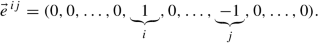
  Clearly $\vec {e}\,^{ij} \in \mathbf 1^{\perp }$ since $\langle \vec {e}\,^{ij}, \mathbf 1 \rangle = 0.$

• (4) Consider the vector $\vec {u}\,^{ij} = {\mathbf {M}}^{-1} (0) \vec {e}\,^{ij} .$

  The vectors $\vec {u}\,^{ij}$ and $\partial \vec {u}\,^{ij} = \vec {e}\,^{ij}$ determine the unique function u on $\Gamma$ satisfying the equation $u'' = 0$ on the edges:

  • u is equal to a linear function with slope $1$ on the path connecting the terminating vertices $i$ and $j$;

  • u is equal to (different) constants on the branches that are left after the path connecting the terminating vertices $V^i$ and $V^j$ is removed from $\Gamma$.

• (5) The distance $d_{ij}$ between the terminating vertices $V^i$ and $V^j$ can be recovered as

  $$\displaystyle \begin{aligned} d_{ij} = u^{ij}_j - u^{ij}_i.\end{aligned}$$

• (6) The distances between all terminating points in a tree determine the tree, as we have already seen in Lemma 20.6.

Thus we have proven

Theorem 20.22 ([237])

The Dirichlet-to-Neumann map ${\mathbf {M}}(0)$ for the standard Laplacian on a finite compact metric tree determines the metric tree uniquely.

References

S. Avdonin, P. Kurasov, Inverse problems for quantum trees. Inverse Probl. Imaging 2(1), 1–21 (2008). https://doi.org/10.3934/ipi.2008.2.1. MR2375320
S. Avdonin, P. Kurasov, M. Nowaczyk, Inverse problems for quantum trees II: recovering matching conditions for star graphs. Inverse Probl. Imaging 4(4), 579–598 (2010). https://doi.org/10.3934/ipi.2010.4.579. MR2726415
M.I. Belishev, Boundary spectral inverse problem on a class of graphs (trees) by the BC method. Inverse Prob. 20(3), 647–672 (2004). https://doi.org/10.1088/0266-5611/20/3/002. MR2067494
M.I. Belishev, On the boundary controllability of a dynamical system described by the wave equation on a class of graphs (on trees). Zap. Nauchn. Sem. S.-Peterburg. Otdel. Mat. Inst. Steklov. (POMI) 308 (2004), no. Mat. Vopr. Teor. Rasprostr. Voln. 33, 23–47, 252. https://doi.org/10.1007/s10958-005-0471-x (Russian, with English and Russian summaries); English transl., J. Math. Sci. (N.Y.) 132(1), 11–25 (2006). MR2092610
M.I. Belishev, A.F. Vakulenko, Inverse problems on graphs: recovering the tree of strings by the BC-method. J. Inverse Ill-Posed Probl. 14(1), 29–46 (2006). https://doi.org/10.1163/156939406776237474. MR2218385
B.M. Brown, R. Weikard, A Borg-Levinson theorem for trees. Proc. R. Soc. Lond. Ser. A Math. Phys. Eng. Sci. 461(2062), 3231–3243 (2005). https://doi.org/10.1098/rspa.2005.1513. MR2172226
H. Gernandt, J. Rohleder, A Calderón type inverse problem for tree graphs. Linear Algebra Appl. 646, 29–42 (2022). https://doi.org/10.1016/j.laa.2022.03.018. MR4403079
P. Kurasov, Can one distinguish quantum trees from the boundary?. Proc. Am. Math. Soc. 140(7), 2347–2356 (2012). https://doi.org/10.1090/S0002-9939-2011-11077-3. MR2898697
V.A. Yurko, Inverse spectral problems for Sturm-Liouville operators on graphs. Inverse Prob. 21(3), 1075–1086 (2005). https://doi.org/10.1088/0266-5611/21/3/017. MR2146822
V.A. Yurko, On the reconstruction of Sturm-Liouville operators on graphs. Mat. Zametki 79(4), 619–630 (2006). https://doi.org/10.1007/s11006-006-0064-0 (Russian, with Russian summary); English transl., Math. Notes 79(3–4), 572–582 (2006). MR2251311
Author information
Authors and Affiliations