
Abstract
Arabica coffee (C. arabica L.) is a highly valued agricultural commodity on the world market. Tons of products are traded internationally, and it has become an extremely valuable resource. However, the species is threatened by the alarmingly low genetic diversity present among its wild populations and agronomic varieties. It is highly relevant to exploit different mechanisms to increase genetic variability in coffee. One of such methods is the induction of variability through chemical or physical mutagenesis. In this work, a population of 320 coffee plants (Coffea arabica L. var. Catuaí) originated from chemically mutagenized embryogenic callus was analysed. Here we describe a protocol for detection of induced mutations using High Resolution Melting (HRM) on a Real Time PCR machine with HRM capabilities. The protocol allows to detect mutations in pooled DNA samples of up to four M2 mutant plants. The procedures and example data are presented for mutation detection in the CaWRKY1 gene. This procedure can be applied for mutation detection in other genes of interest to coffee breeders and scientists.
You have full access to this open access chapter, Download chapter PDF
Keywords
1 Introduction
The genetic improvement of crops depends on the selection of genotypes with the desired, novel agronomic characteristics. Genetic variation provides the main resource to develop varieties adapted to different scenarios. Arabica coffee (Coffea arabica L.) is an allopolyploid species (2n = 4x = 44) that resulted from hybridization between two species extremely close to C. eugenioides and C. canephora (Scalabrin et al. 2020). The genetic variation present in Arabica coffee doesn’t represent the entire possible conglomerate of spontaneous mutations. Rather, they result from the recombination of genotypes within populations and their continuous interaction with both biotic and abiotic environmental elements (Oladosu et al. 2016). Therefore, the availability of genotypes to introduce into a breeding program is limited.
Through induced mutagenesis it is possible to generate heritable changes in the genome of an organism, without the need for genetic segregation or recombination (Oladosu et al. 2016). These changes can be generated in genes that regulate characteristics of interest and finally allow their improvement or functional analysis. Mutation induction has been carried out in different tissue types through irradiation and exposure to chemical agents (Serrat et al. 2014). One of the most widely used chemical agents, is ethyl methanesulfonate (EMS), which mainly induces C-T substitutions that result in C/G to A/T transitions (Kim et al. 2006).
A fundamental aspect of the genetic improvement through induced mutagenesis is the process of identifying those plants with the mutations of interest in their genome. This can be done in two phases: 1) screening or detection of the mutants, and 2) confirmation of the mutation (Forster and Shu 2012). To achieve this, it is important to have an efficient and scalable detection strategy to increase the probability of detecting new genetic variants within mutant populations. The High-Resolution Melting (HRM) analysis can facilitate the detection of variants in genes. This technique does not involve any enzymes, but rather requires the presence of saturating fluorochromes that interact with the double-stranded DNA. In this way, a heteroduplex structure, with less stability, is denatured at lower temperatures than the DNA copies, a process that is monitored by the decrease in fluorescence emission (Szurman-Zubrzycka et al. 2016). When trying to detect mutations in large populations, it is convenient to pool the DNA of individuals, thus reducing the number of samples to be analyzed and consequently the cost. However, this clustering decreases the sensitivity and makes it difficult to detect low frequency mutations (Simko 2016). COLD-PCR (lower denaturation temperature co-amplification) can be applied to increase the sensitivity of HRM analysis by preferentially amplifying mismatched DNA. This is a modification of PCR where the reaction is carried out at a denaturation temperature at which the heteroduplex DNA is denatured in a greater proportion than the other DNA types (Chen and Wilde 2011). This chapter describes the PCR-HRM based detection of variants in genomic sequences of Arabica coffee plants var. Catuaí developed via chemical mutagenesis.
2 Materials
2.1 Plant Material
-
1.
M2 mutant coffee population (e.g., Coffea arabica L. var. Catuaí) (see Fig. 1a see Note 1).
Fig. 1 
Coffee (Coffea arabica L. var. Catuaí) M2 mutant population. a M2 mutant plants in the experimental field, b fresh material brought from the field to the lab for DNA extraction, c young and disease-free leaves used for DNA extraction

2.2 Reagents
-
1.
1 Kb DNA ladder (e.g., Thermo Scientific Cat Nr.: SM0311).
-
2.
18S primers (18S_F: 5′-AGGTAGTGACAATAAATAACAA-3′ and 18S_R: 5′-TTTCGCAGTTGTTCGTCTTTC-3′) (see Note 2).
-
3.
6X loading dye (e.g., Thermo Scientific Cat Nr.: R0611).
-
4.
Agarose (e.g., Phytotechnology Cat Nr.: A110).
-
5.
Chloroform (e.g., Sigma Cat Nr.: 288306) (see Note 3).
-
6.
dNTPs (25 mM each) (e.g., Thermo Scientific Cat Nr.: R1121).
-
7.
EDTA (e.g., Phytotechnology Cat Nr.: E582).
-
8.
Ethanol (e.g., Sigma Cat Nr.: 459844).
-
9.
GelRed™ (e.g., Gold Biotechnology, Inc Cat Nr.: G-720-500).
-
10.
Hexadecyltrimethylammonium bromide (CTAB) (e.g., Bio Basic Inc. Cat Nr.: CB0108).
-
11.
Isopropanol (e.g. Sigma Cat Nr.: I9516).
-
12.
MeltDoctor™ HRM Master Mix (e.g., Thermo Scientific Cat Nr.: 4415440).
-
13.
2-Mercaptoethanol (e.g., Phytotechnology Cat Nr.: M649).
-
14.
Mix for real-time PCR with HRM (e.g., Melt Doctor™, Thermo Scientific Cat Nr.: 4415440).
-
15.
NaCl (e.g., Sigma Cat Nr.: S9888).
-
16.
Phenol (e.g., Sigma Cat Nr.: P1037).
-
17.
Polyvinylpyrrolidone (PVP-40) (e.g., Phytotechnology Cat Nr.: P728).
-
18.
RNAase (10 mg/mL) (e.g., Thermo Scientific Cat Nr.: EN0531).
-
19.
Taq DNA polymerase recombinant (5 U/μl) (e.g., Thermo Scientific Cat Nr.: EP0402).
-
20.
TBE buffer (5X) (e.g., Phytotechnology Cat Nr.: T773).
-
21.
Tris-HCl (pH 8.0) (e.g., Phytotechnology Cat Nr.: T764).
2.3 Equipment
-
1.
Analytical balance.
-
2.
Autoclave.
-
3.
High-resolution real-time PCR instrument (e.g., CFX96 real-time PCR system, Bio-Rad Laboratories, Hercules, CA, USA).
-
4.
Electrophoresis apparatus (electrophoresis tank and power supply).
-
5.
Freezer (− 20 °C).
-
6.
Gel imaging documentation system.
-
7.
High-resolution real-time PCR instrumentation.
-
8.
Hot plate shaker.
-
9.
Microwave.
-
10.
PCR workstation with UV light.
-
11.
pH meter.
-
12.
Refrigerated centrifuge.
-
13.
Spectrophotometer (e.g., NanoDrop 2000, Thermo Scientific, Osterode am Harz, Germany).
-
14.
Thermal cycler.
-
15.
Thermomixer block.
-
16.
Vortex stirrer.
-
17.
Water bath.
2.4 Software
-
1.
Precision Melt Analysis™ Software (CFX96 real-time PCR system, Bio-Rad Laboratories, Hercules, CA, USA).
-
2.
Molecular Evolutionary Genetics Analysis (MEGA) (https://www.megasoftware.net/).
3 Methods
3.1 Preparation of Stock Solutions
-
1.
100 mL extraction buffer: add 10.0 mL 1 M Tris/HCl (pH 8.0), 28.0 mL 5 M NaCl, 4.0 mL 0.5 M EDTA (pH 8.0), 2 g CTAB, 2 g PVP and dissolve by adding 58.0 mL of molecular grade water (see Note 4). Once completely dissolved, add 40 μL of 2-mercaptoethanol for each 20 mL of extraction buffer.
-
2.
1X TE [10 mM Tris/HCl (pH 8.0) containing 1 mM EDTA (pH 8.0)]: add 1.0 mL Tris/HCl (1 M, pH 8.0) and 0.2 mL EDTA (0.5 M, pH 8.0) and molecular grade water to a final volume of 100 mL.
-
3.
Chloroform:phenol (24:1): in a ducted chemical fume hood, combine 48 mL chloroform with 2 ml phenol (pH 8.0) in a 100 mL glass bottle with a lid.
3.2 DNA Extraction
The following protocol describes the procedure for the extraction of genomic DNA from young and disease-free coffee leaves. It has been optimized to eliminate or reduce oxidation during the extraction. Although it can be used on dry material, the recommendation is to use fresh tissue, which yields better quality DNA. To transfer the fresh material from the field to the lab, it is recommended to cut the branch and place it in a bag with water until it reaches the laboratory (see Fig. 1b).
-
1.
Place approx. 50 mg fresh weight plant material in a 2 mL reaction tube (see Fig. 1c).
-
2.
Add 600 µL of extraction buffer, macerate by hand using mortar and pestle until the samples are homogeneous and mix with the vortex.
-
3.
Incubate the sample at 65ºC for 12 min, every 6 min invert the tubes about 5 times.
-
4.
Add 600 µL of chloroform:phenol (24:1) in the ducted chemical fume hood (see Note 5).
-
5.
Mix by inversion 15 times. Do not use vortex at this stage.
-
6.
Centrifuge the sample for 5 min at 13,000 rpm, at 4 °C.
-
7.
Transfer 350 µL of the supernatant to a new 1.5 mL reaction tube. Be careful not to contaminate the tip with the organic phase (bottom phase).
-
8.
Add 350 µL of a cold isopropanol, shake 20 times by inversion and incubate 15 min at − 20 °C.
-
9.
Centrifuge the sample for 7 min at 13,000 rpm, at 4 °C.
-
10.
Discard the supernatant by decanting. Be careful not to lose the pellet.
-
11.
Add 500 µl of cold 70% v/v ethanol.
-
12.
Centrifuge the sample for 2 min at 13,000 rpm, at 4 °C.
-
13.
Carefully remove the ethanol by decanting. Be careful not to lose the pellet.
-
14.
Dry the pellet at 45ºC until there are no ethanol residues.
-
15.
Resuspend the pellet in 50 µl of 1X TE.
-
16.
Add 1 µL of RNase (conc. stock solution 10 mg/mL).
-
17.
Incubate for 30 min at 37 °C.
-
18.
Store at − 20 °C.
3.3 Determination of DNA Integrity
-
1.
Weigh 0.8 g agarose.
-
2.
Mix agarose with 100 mL 1X TBE in a flask.
-
3.
Microwave for 1–2 min until the agarose is completely dissolved, avoid boiling the solution.
-
4.
Let the agarose solution cool down for about 5 min.
-
5.
Add 2 μl of GelRed™ solution per 100 mL gel.
-
6.
Pour the gel slowly avoiding any air bubbles.
-
7.
Once solidified, place the agarose gel into an electrophoresis tank filled with 1XTBE.
-
8.
Add 6X loading buffer to each DNA sample at a final concentration of 1X (e.g., 2 μL 6X loading dye + 5 μL DNA + 5 μL molecular grade water).
-
9.
Load 2–3 μL of a molecular weight ladder (e.g., 1 Kb DNA Ladder) in the first and last lane of the gel.
-
10.
Load your samples into the remaining wells.
-
11.
Run the gel at 100 V for about 45–60 min or until the dye has migrated approximately 75–80% in the gel.
-
12.
Visualize the DNA fragments using a gel imaging device (see Fig. 2a).
Fig. 2 
Quantification and determination of DNA integrity, a DNA isolated from young and disease-free leaves. L: 1 Kb DNA Ladder, 1–6: samples, b quantification and DNA purity determined using a NanoDrop 2000 (Thermo Scientific) spectrophotometer, c PCR amplification of a 480 bp fragment of the 18S gene L: 100 bp DNA Ladder, 1–6: samples
-
13.
Quantify the concentration of the DNA using the NanoDrop 2000 spectrophotometer (see Fig. 2b and Note 6).

3.4 PCR Amplification of the 18S Gene
-
1.
Thaw reagents on ice, vortex and centrifuge prior use.
-
2.
Prepare a MastexMix by pipetting on ice the following components in a final volume of 25 μl: 1X Taq PCR buffer, 0.25 mM of each dNTPs, 0.2 μM of each primer, 1.5 mM of MgCl2, 0.5 U Taq polymerase, and 1 μl DNA (100 ng/μl). Include a negative control (no-DNA template) (see Notes 7 and 8).
-
3.
Place the tubes in the thermal cycler with the following program: 95 °C for 10 min followed by 30 cycles at 94 °C for 30 s, 53 °C for 30 s, 72 °C for 90 s and a final step of 72 °C for 10 min.
-
4.
Prepare a 1.5% m/v agarose gel in 1X TBE as described previously (see Sect. 3.3).
-
5.
Load 15 µl of the PCR product on the gel.
-
6.
Run at 100 V for 1 h.
-
7.
A PCR product of approximately 481 bp should be visible (see Fig. 2c).
-
8.
Record the amplification of the 18S gene.
3.5 Literature Mining and Selection of Candidate Genes for Mutation Screening
-
1.
Go to PubMed database (http://www.ncbi.nlm.nih.gov/pubmed/) (see Fig. 3, step 1).
Fig. 3 
Literature mining and selection of candidate genes for mutation screening. For details see Sect. 3.5
-
2.
Enter the desired word combination associated with a particular topic, e.g., “coffee and rust resistance genes” (see Fig. 3, step 2).
-
3.
Click on “Search” (see Fig. 3, step 3).
-
4.
Filter the results in terms of article type, text availability, publication date or investigated species (see Fig. 3, step 4).
-
5.
Click on the “Abstract” of the desired article (see Fig. 3, step 5).
-
6.
Select ‘Related information’ menu within abstract content to link to other related NCBI databases for the selected record (e.g., gene and protein sequence) (see Fig. 3, step 6).
-
7.
Retrieve gene and protein sequence (see Fig. 3, step 7).

3.6 Primer Design
-
1.
Go to Primer3 primer design tool (version 4.1.0) (Primer3 Input) (see Fig. 4, step 1).
-
2.
Paste a raw nucleotide sequence (5′–3′) of your gene target in the box, e.g., CaWRKY1 (GenBank: DQ335599.1) (see Fig. 4, step 2 and Note 9).
Fig. 4 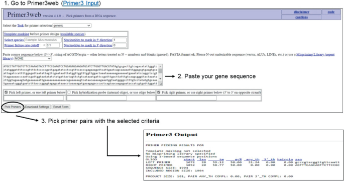
Designing primers for the amplification of a specific gene fragment using Primer3. For details see Sect. 3.6
-
3.
Design primers for HRM analysis with the following criteria:
-
A length of 18–25 nucleotides.
-
The melting temperature (Tm) between 55 and 65 °C, and not more than 3 °C difference of each other.
-
The GC content between 40 and 60%, with the 3′ of a primer ending in C or G to promote binding.
-
Balanced distribution of GC-rich and AT-rich domains.
-
Lack of runs of four or more of one base or dinucleotide repeats.
-
Lack of intra-primer homology (more than three bases that complement within the primer) or inter-primer homology (forward and reverse primers having complementary sequences).
-
-
4.
Click ‘Pick Primers’ command to obtain primer pairs which best match the selected criteria (see Fig. 4, step 3).
-
5.
Check the absence of secondary structures and properties of designed primers using appropriate software, e.g., the Oligo Analyser™ tool (https://www.idtdna.com/pages/tools/oligoanalyzer).
-
6.
For each primer pairs, complete the information shown in Table 1.
Table 1 Properties of designed primers. Example primers designed for the CaWRKY1 gene -
7.
Order primer pairs through a specialized company (e.g., Macrogen, South Korea).

3.7 In Silico Analysis of Primer Specificity
-
1.
Go to National Centre for Biotechnology Information (NCBI) database (https://www.ncbi.nlm.nih.gov/) (see Fig. 5, step 1).
Fig. 5 
Primer specificity in silico analysis performed at NCBI. For details see Sect. 3.7
-
2.
Click “BLAST” button (see Fig. 5, step 2).
-
3.
Choose the type of BLAST based on your goal. In our case, we chose “Nucleotide BLAST” (see Fig. 5, step 3).
-
4.
Paste the primer sequences in the box, e.g., CaWRKY1_F: 5-TGAGTATGTTTCCGGCCACC-3 (see Fig. 5, step 4).
-
5.
Select “Somewhat similar sequences (blastn)” (see Fig. 5, step 5).
-
6.
Click “BLAST” button (see Fig. 5, step 6).
-
7.
Check the E-value (see Note 10), percentage identity (see Note 11) and query cover (see Note 12) of the designed primer pairs (see Fig. 5, step 7).

3.8 In Silico PCR
-
1.
Access Primer BLAST at NCBI (https://www.ncbi.nlm.nih.gov/tools/primer-blast/index.cgi) (see Fig. 6, step 1).
Fig. 6 
In silico PCR analysis performed at NCBI. For details see Sect. 3.8
-
2.
Paste the gene sequence in FASTA format and your designed primer pairs (see Fig. 6, step 2).
-
3.
Scroll down and enter an organism name (Coffea arabica (taxid:13443) (see Fig. 6, step 3).
-
4.
Click “Get primers” button (see Fig. 6, step 4).
-
5.
Check product length, Tm, GC%, and self-complementarity (see Fig. 6, step 5).

3.9 Nested PCR
-
1.
Prepare fourfold DNA pools that will serve as the template for HRM-PCR reactions. DNA from each of four M2 individuals should be mixed in equal amounts to obtain a final concentration of 30 ng/μl.
-
2.
Prepare a Master Mix by pipetting on ice the following components in a final volume of 25 μl: 1X Taq PCR buffer, 0.25 mM of each dNTPs, 0.2 μM of each primer, 1.5 mM of MgCl2, 1.5 U Taq polymerase, and 1 μl DNA (90 ng/μl). Include a negative control, as well as a no-DNA template.
-
3.
Before placing the tubes in the instrument, briefly spin for 10 s at room temperature.
-
4.
Place the tubes in the thermal cycler with the following touch down program: 95 °C for 10 min followed by a touch down phase consisting of 13 cycles at 95 °C for 60 s, 65–53 °C for 60 s, 72 °C for 120 s and a final amplification phase involving 12 cycles at 95 °C for 60 s, 53 °C for 60 s, 72 °C for 120 s and a final 72 °C for 10 min.
-
5.
Confirm the specific amplification of each product by agarose gel electrophoresis.
3.10 Mutation Identification Using the HRM Technique
The mutation identification using PCR-HRM was performed using the nested PCR methodology.
-
1.
Design the plate following the steps defined by the software (e.g., HRM Software, Applied Biosystems ™) (see Fig. 7a).
Fig. 7 
Mutation identification using the HRM technique, a example of an HRM-PCR plate, b example of an HRM-PCR program of temperatures with melt curve protocol adjusted for posterior analysis
-
2.
Prepare a Master Mix by pipetting on ice the following components in a final volume of 10 μl: 5 μl Melt Doctor™ HRM Master Mix, 0.4 μM of each primer, 2 mM MgCl2 and PCR molecular grade water. Include a negative control (no-DNA template).
-
3.
Distribute 9 μL of the reaction mix into each well or tube and add 1 μL of the nested PCR product (1:1000 dilution).
-
4.
Place the tubes or plate in the high-resolution real-time PCR instrument and set the program as follows (see Fig. 7b):
-
Initial denaturation: 95 °C for 10 min.
-
Amplification (30 cycles): 95 °C for 30 s, 57 °C for 15 s, and 72 °C for 20 s
-
High-resolution melting:
-
Formation of homo- and heteroduplexes: 95 °C for 30 s, 40 °C for 60 s with continuous fluorescence acquisition (60–95 °C).
-
-
-
5.
Close wells/tubes. Spin down to ensure that the entire volume is at the bottom of the tubes.
-
6.
Place the reaction tubes in the thermal cycler and start the run.
-
7.
After finishing the real-time PCR, open the precision melt analysis software and save the generated melt file (see Fig. 8).
Fig. 8 
Example of a melt file generated with the precision melt analysis, showing the normalized melt curve, the difference curve, the plate, and the classification of species by cluster
-
8.
Open the melt file and analyse the results (see Note 13).


3.11 DNA Sanger Sequencing for HRM Validation
-
1.
Confirm a potential mutation by Sanger sequencing the fragment being analysed for the identified M2 individuals.
-
2.
Check the quality of electropherograms using for example MEGA software.
-
3.
Analyse the sequencing results using the NovoSNP 3.0.1 program (Weckx et al. 2005).
4 Notes
-
1.
This protocol has been established using a M2 mutant population obtained from mutagenized M0 coffee seeds (Coffea arabica L. var. Catuaí). It can be used as a reference for other coffee varieties, nevertheless, it is recommended to optimize the HRM-PCR parameter for each variety used.
-
2.
PCR amplification of the 18S endogenous gene is used as internal control for PCR evaluation of the quality and integrity of extracted plant DNA.
-
3.
Read the Materials Safety Data Sheet (MSDS) of the reagents being used and follow the recommendation of the manufacturer. It is very important to wear personal protective equipment (gloves, safety glasses with side shields or chemical goggles; lab coat, closed-toe shoes, and full-length pants).
-
4.
Prepare all solutions using ultrapure molecular grade water (deionized water) and analytical grade reagents.
-
5.
DNA extraction should be performed in a dedicated molecular biology laboratory equipped with a ducted fume hood, toxic waste disposal and decontamination procedures.
-
6.
The ratio of absorbance at 260 and 280 nm is used to assess the purity of DNA. A ratio of ~ 1.8 is generally accepted as “pure” for DNA. Moreover, the ratio 260/230 is used as a secondary measure of nucleic acid purity; 260/230 values in the range of 2.0–2.2 indicate the absence of contaminants (such as carbohydrates and phenol).
-
7.
Use molecular biology grade consumables (e.g., tips, reaction tubes, PCR tubes, real-time PCR strips and caps) for DNA extraction and PCR analysis (sterile, DNase and RNase free). Other materials and consumables can be purchased in non-sterile conditions and autoclaved (121 °C, 15 min) before use.
-
8.
To avoid cross contamination, it is highly recommended to work in a PCR workstation, especially when performing all tasks associated with the preparation of PCR or HRM-PCR mixes.
-
9.
The genomic regions of the CaKO, CaPOP, CaWRKY1, CCoAOMT1, ITS2, LOX1, SUS2, ABC, and FLC genes were selected based on the potential effect that a variation could have on certain phenotypes of C. arabica L. plants.
-
10.
The Expected value (E value) is a parameter that describes the number of hits one can “expect” to see by chance when searching a database of a particular size. The lower the E-value, or the closer it is to zero, the more “significant” the match is.
-
11.
The percent identity is a number that describes how similar the query sequence is to the target sequence (how many characters in each sequence are identical). The higher the percent identity is, the more significant the match.
-
12.
The query cover is a number that describes how much of the query sequence is covered by the target sequence. If the target sequence in the database spans the whole query sequence, then the query cover is 100%. This tells us how long the sequences are, relative to each other.
-
13.
The Precision Melt Analysis™ Software uses predefined automated parameters, which might be adjusted according to the type of analysis that is being processed. See the user guide for more details (https://www.bio-rad.com/sites/default/files/webroot/web/pdf/lsr/literature/10000080911.pdf).
References
Chen Y, Wilde HD (2011) Mutation scanning of peach floral genes. BMC Plant Biol 11:1–8
Forster BP, Shu QY (2012) Plant mutagenesis in crop improvement: basic terms and applications. In: Shu QY, Forster BP, Nakagawa H (eds) Plant mutation breeding and biotechnology. CABI, Wallingford, pp 9–20
Kim Y, Schumaker KS, Zhu JK (2006) EMS mutagenesis of Arabidopsis. Methods Mol Biol 323:101–103
Oladosu Y, Rafii MY, Abdullah N, Hussin G, Ramli A, Rahim HA, Usman M (2016) Principle and application of plant mutagenesis in crop improvement: a review. Biotechnol Biotechnol Equip 30:1–16
Scalabrin S, Toniutti L, Di Gaspero G, Scaglione D, Magris G, Vidotto M, Bertrand B (2020) A single polyploidization event at the origin of the tetraploid genome of Coffea arabica is responsible for the extremely low genetic variation in wild and cultivated germplasm. Sci Rep 10:1–13
Serrat X, Esteban R, Guibourt N, Moysset L, Nogués S, Lalanne E (2014) EMS mutagenesis in mature seed-derived rice calli as a new method for rapidly obtaining TILLING mutant populations. Plant Methods 10. https://doi.org/10.1186/1746-4811-10-5
Simko I (2016) High-resolution DNA melting analysis in plant research. Trends Plant Sci 21:528–536
Szurman-Zubrzycka M, Chmielewska B, Gajewska P, Szarejko I (2016) Mutation detection by analysis of DNA heteroduplexes in TILLING populations of diploid species. In: Jankowicz-Cieslak J, Tai T, Kumlehn J, Till B (eds) Biotechnologies for plant mutation breeding. International Atomic Energy Agency. Springer Open, pp 292–303
Weckx S, Del-Favero J, Rademakers R, Claes L, Cruts M, De Jonghe P, Van Broeckhoven C, De Rijk P (2005) novoSNP, a novel computational tool for sequence variation discovery. Genome Res 15(3):436–442. https://doi.org/10.1101/gr.2754005
Acknowledgements
Funding for this work was provided by the University of Costa Rica, the Ministerio de Ciencia, Tecnología y Telecomunicaciones (MICITT), the Consejo Nacional para Investigaciones Científicas y Tecnologicas (CONICIT) (project No. 111-B5-140; FI-030B-14) and a fellowship granted to Alejandro Bolivar-González by Centro Nacional de Alta Tecnología (CeNAT). A. Gatica-Arias acknowledged the Cátedra Humboldt 2023 of the University of Costa Rica for supporting the dissemination of biotechnology for the conservation and sustainable use of biodiversity.
Author information
Authors and Affiliations
Corresponding author
Editor information
Editors and Affiliations
Rights and permissions
Open Access This chapter is licensed under the terms of the Creative Commons Attribution 4.0 International License (http://creativecommons.org/licenses/by/4.0/), which permits use, sharing, adaptation, distribution and reproduction in any medium or format, as long as you give appropriate credit to the original author(s) and the source, provide a link to the Creative Commons license and indicate if changes were made.
The images or other third party material in this chapter are included in the chapter's Creative Commons license, unless indicated otherwise in a credit line to the material. If material is not included in the chapter's Creative Commons license and your intended use is not permitted by statutory regulation or exceeds the permitted use, you will need to obtain permission directly from the copyright holder.
Copyright information
© 2023 The Author(s)
About this chapter

Cite this chapter
Gatica-Arias, A., Bolívar-González, A., Sánchez-Barrantes, E., Araya-Valverde, E., Molina-Bravo, R. (2023). High Resolution Melt (HRM) Genotyping for Detection of Induced Mutations in Coffee (Coffea arabica L. var. Catuaí). In: Ingelbrecht, I.L., Silva, M.d.C.L.d., Jankowicz-Cieslak, J. (eds) Mutation Breeding in Coffee with Special Reference to Leaf Rust. Springer, Berlin, Heidelberg. https://doi.org/10.1007/978-3-662-67273-0_20
Download citation
DOI: https://doi.org/10.1007/978-3-662-67273-0_20
Published:
Publisher Name: Springer, Berlin, Heidelberg
Print ISBN: 978-3-662-67272-3
Online ISBN: 978-3-662-67273-0
eBook Packages: Biomedical and Life SciencesBiomedical and Life Sciences (R0)