Dual System Encryption Framework in Prime-Order Groups via Computational Pair Encodings

Abstract

We propose a new generic framework for achieving fully secure attribute based encryption (ABE) in prime-order bilinear groups. Previous generic frameworks by Wee (TCC’14) and Attrapadung (Eurocrypt’14) were given in composite-order bilinear groups. Both provide abstractions of dual-system encryption techniques introduced by Waters (Crypto’09). Our framework can be considered as a prime-order version of Attrapadung’s framework and works in a similar manner: it relies on a main component called pair encodings, and it generically compiles any secure pair encoding scheme for a predicate in consideration to a fully secure ABE scheme for that predicate. One feature of our new compiler is that although the resulting ABE schemes will be newly defined in prime-order groups, we require essentially the same security notions of pair encodings as before. Beside the security of pair encodings, our framework assumes only the Matrix Diffie-Hellman assumption (Escala et al., Crypto’13), which includes the Decisional Linear assumption as a special case.

Recently and independently, prime-order frameworks are proposed also by Chen et al. (Eurocrypt’15), and Agrawal and Chase (TCC’16-A). The main difference is that their frameworks can deal only with information-theoretic encodings, while ours can also deal with computational ones, which admit wider applications. We demonstrate our applications by obtaining the first fully secure prime-order realizations of ABE for regular languages, ABE for monotone span programs with short-ciphertext, short-key, or completely unbounded property, and ABE for branching programs with short-ciphertext, short-key, or unbounded property.

Keywords

1 Introduction

Attribute based encryption (ABE), initiated by Sahai and Waters [40], is an emerging paradigm that extends beyond normal public-key encryption. In an ABE scheme for predicate $R:\mathbb {X}\times \mathbb {Y}\rightarrow \{0,1\}$, a ciphertext is associated with a ciphertext attribute, say, $Y \in \mathbb {Y}$, while a key is associated with a key attribute, say, $X \in \mathbb {X}$, and the decryption is possible if and only if $R(X,Y)=1$.¹ In Key-Policy (KP) type, $\mathbb {X}$ is a set of Boolean functions (often called policies), while $\mathbb {Y}$ is a set of inputs to functions, and we define $R(f,x)=f(x)$. Ciphertext-Policy (CP) type is the dual of KP where the roles of $\mathbb {X}$ and $\mathbb {Y}$ are swapped (that is, policies are associated to ciphertexts). Besides direct applications of fine-grained access control [21], ABE is also known to imply verifiable computation outsourcing [38].

The standard security requirement for ABE is full security, where an adversary is allowed to adaptively query keys for any attribute X as long as $R(X,Y)=0$, where Y is an adversarially chosen attribute for a challenge ciphertext. Dual system encryption techniques introduced by Waters [44] have been successful approaches for constructing fully secure ABE systems that are based on bilinear groups. Despite being versatile as they can be applied to ABE systems for many predicates, until only recently, however, there were no known generic frameworks that can use the techniques in a black-box and modular manner. Wee [46] and Attrapadung [3] recently proposed such generic frameworks that abstract the dual system techniques by decoupling what seem to be essential underlying primitives and characterizing their sufficient conditions so as to obtain fully-secure ABE automatically via generic constructions. However, their frameworks are inherently constructed over bilinear groups of composite-order. Although composite-order bilinear groups are more intuitive to work with, especially in the case of dual system techniques, prime-order bilinear groups are more preferable as they provide more efficient and compact instantiations. This has been motivated already in a line of research [18, 22, 24, 28, 29, 34, 36, 41]. More concretely, group elements in composite-order groups are more than 12 times larger than those in prime-order groups for the same security level (3072 bits or 3248 bits for composite-order vs 256 bits for prime-order in case of 128-bit security, according to NIST or ECRYPT II recommendations [22]). Regarding time performances, Guillevic [22] reported that bilinear pairings are 254 times slower in composite-order than in prime-order groups for the same 128-bit security. Moreover, exponentiations are also more than 200 times slower [22, Table 6]. In this work, our goal is to propose a generic framework for dual-system encryption in prime-order groups.

The generic frameworks of [3, 46] work similarly but with the difference that the latter [3] captures also dual system techniques with computational approaches, which are generalized from techniques implicitly used in the ABE of Lewko and Waters [32]. (The former [46] only captures the traditional dual systems, which implicitly use information-theoretic approaches). Using computational approaches, the framework of [3] is able to obtain the first fully secure schemes for many ABE primitives for which only selectively secure constructions were known before, including KP-ABE for regular languages [45], KP-ABE for Boolean formulae² with constant-size ciphertexts [9], and (completely) unbounded KP-ABE for Boolean formulae [31, 39]. Moreover, Attrapadung and Yamada [10] recently show that, within the framework of [3], we can generically convert ABE to its dual scheme, i.e., key-policy to ciphertext-policy type, and vice versa. They also show a conversion to its dual-policy [8] type, which is the conjunctive of KP and CP. Many instantiations were then obtained in [10], including the first CP-ABE for formulae with short keys. We therefore choose to build upon [3].

1.1 Our Contributions on Framework

New Framework. We present a new generic framework for achieving fully secure ABE in prime-order groups. It is generic in the sense that it can be applied to ABE for arbitrary predicate. Our framework extends the framework of [3], which was constructed in composite-order groups, and works in a similar manner as follows. First, the main component is a primitive called pair encoding scheme defined for a predicate. Second, we provide a generic construction that compiles any secure pair encoding scheme for a predicate R to a fully secure ABE scheme for the same predicate R. The security requirement for the underlying encoding scheme is exactly the same as that in the framework of [3]; in particular, our framework can deal with both information-theoretic and computational encodings. On the other hand, we restrict the syntax of encodings into a class we call regular encodings, via some simple requirements. This confinement, however, seems natural and does not affect any concrete pair encoding schemes proposed so far [3, 10, 46]. Beside the security of pair encodings, our framework assumes only the Matrix Diffie-Hellman assumption [17], which includes the Decisional Linear assumption as a special case.

Conceptually, since our framework uses the same security requirement for pair encodings as in the composite-order framework of [3], we can view it as an automatic way for translating ABE from composite-order to prime-order settings.

Prime-order frameworks are recently and independently proposed by Chen, Gay, and Wee [14] and Agrawal and Chase [2], albeit they can deal only with information-theoretic encodings. We compare them later in Sect. 1.4. As a side result, we also simplify our scheme using a simpler basis from [14] in Sect. 8.

1.2 Our Contributions on Instantiations

New Instantiations (the First in Prime-order Settings). By using exactly the same encoding instantiations in [3, 10], we automatically obtain fully secure ABE schemes, for the first time in prime-order groups, for various predicates:

• KP-ABE and CP-ABE for regular languages,

• KP-ABE for monotone span programs with constant-size ciphertexts,

• CP-ABE for monotone span programs with constant-size keys,

• Completely unbounded KP-ABE and CP-ABE for monotone span programs.

The assumptions for respective encodings are the same as those in [3] (albeit with a minor syntactic change to prime-order groups); some are parameterized assumptions (or often called q-type), as in [3]. Moreover, via the dual-policy conversion of [10], we also obtain their respective dual-policy variants.

We give their detailed comparisons in Tables 5, 6 in Sect. 7. Here, for high-level overview, we position our instantiations in Table 2, which show prime-order schemes by their properties. In Table 2, our instantiations that are the first such schemes for given predicates and properties are specified by New. Our new instantiations that are not the first of a kind are specified by $\mathbf{New }'$. Table 1 provides composite-order schemes for comparison.

Table 1. Composite-order ABE, positioned by properties (for comparing to Table 2)

Table 2. Prime-order ABE schemes, positioned by properties

First Realizations. We also obtain the first-ever realizations of ABE for some predicates, namely,

• Unbounded KP-ABE and CP-ABE for branching programs (BP),

• KP-ABE for branching programs with constant-size ciphertexts,

• CP-ABE for branching programs with constant-size keys.

Unbounded ABE-BP refers to a system that allows an encryptor to associate a ciphertext with an input string of any length (in the case of KP). All of our above ABE-BP schemes are the first such schemes for respective variants even among composite-order or selectively secure schemes. Comparing to the previous schemes, KP-ABE-BP of [14, 19, 25] are of bounded type and require linear-size ciphertexts and keys³, while (selective) KP-ABE-BP of [20] achieves short keys. We obtain our above ABE-BP schemes by invoking the theorem stating a generic implication from ABE for monotone span programs (MSP) to ABE-BP (see Remark 6 for further discussion on this theorem).

Update after Subsequent Work. Subsequent to our work, Attrapadung et al. [7] present various conversions for ABE. By applying their conversions to some of our instantiations, they obtain CP-ABE with short ciphertexts and KP-ABE with short keys for (non-)monotone span programs. Now, by applying the ABE-MSP-to-ABE-BP conversion back to their instantiations, we obtain further (fully secure) schemes not explicitly achievable before, namely:

• KP-ABE for branching programs with constant-size keys,

• CP-ABE for branching programs with constant-size ciphertexts.

Moreover, we can combine KP-ABE and CP-ABE both with short keys to DP-ABE with short keys. The same goes for short ciphertexts. We mark the schemes after this update as $\mathbf{Newer }_i$ in Table 2. Interestingly, all of our results complete the whole Table 2, which had been otherwise filled with open problems before.

1.3 Our Techniques

Due to the lack of space, we defer a more detailed discussion on our techniques to the full version [4]. We provide only a summary here.

Background on [3]. We first briefly review the framework of [3]. In the generic construction of [3], a ciphertext ${\mathsf {CT}}$ encrypting M, and a key $\mathsf {SK}$ take the forms:

$$\begin{aligned} {\mathsf {CT}}&= ({\varvec{C}},C_0) = (g_1^{{\varvec{c}}({\varvec{s}},{\varvec{h}})},\, M e(g_1,g_2)^{\alpha s_0}),&\mathsf {SK}&= g_2^{{\varvec{k}}(\alpha , {\varvec{r}},{\varvec{h}})} \end{aligned}$$

where ${\varvec{c}}$ and ${\varvec{k}}$ are encodings of attributes Y and X associated to a ciphertext and a key, respectively. Here, $g_1,g_2$ are generators of subgroups of order $p_1$ of $\mathbb {G}_1,\mathbb {G}_2$, which are asymmetric bilinear groups of composite order $N=p_1p_2p_3$ with bilinear map $e:\mathbb {G}_1\times \mathbb {G}_2\rightarrow \mathbb {G}_T$. The bold fonts denote vectors. Intuitively, $\alpha$ plays the role of a master key, ${\varvec{h}}$ represents common variables (or called parameters). These define a public key $\mathsf {PK}=(g_1^{{\varvec{h}}}, e(g_1,g_2)^{\alpha })$. ${\varvec{s}},{\varvec{r}}$ represents randomness in the ciphertext and the key, respectively, with $s_0$ being the first element in ${\varvec{s}}$. The pair $({\varvec{c}},{\varvec{k}})$ form a pair encoding scheme for predicate R. Informally, the main theorem of [3] states that if the pair encoding is secure and subgroup decision assumptions hold, then the ABE scheme (with ${\mathsf {CT}},\mathsf {SK}$ as above) is fully secure.

Our Approach. Towards translating to a new prime-order based framework, we identify a set of features consisting of element representations, procedures, properties, and assumptions that are required by the framework of [3]. We list up the first three categories in Sect. 4.

As for assumptions, our goal is to use the security definition of pair encoding “as is”, since this will allow us to instantly instantiate the encoding schemes already proposed and proved secure in [3]. If we can leave encoding “as is”, we will only have to replace subgroup decision assumptions provided by composite-order groups with some mechanisms from prime-order groups that mimic them.

Candidate Techniques. There are two candidate tools for simulating subgroup decision in prime-order groups: Dual Pairing Vector Space (DPVS) [28, 35, 36] and Prime-order Dual System Group (PDSG) [15]. We argue (in the full version [4]) that DPVS would require modifying one of the encoding (in the pair encoding) to an “orthogonal form” in order to enable inner-product spaces, which seems essential in this approach. This, however, would violate our goal to use encoding “as is”. We thus turn to use the other tool: PDSG. Although PDSG was devised for specific predicates such as HIBE in the first place [15], it seems compatible to the pair encoding syntax in terms of element representations since, roughly speaking, it provides one-to-one translation of elements. (This itself is although implicit in [15]). Intuitively, each $\mathbb {Z}_N$ element in ${\varvec{s}},{\varvec{r}},{\varvec{h}}$ is mapped to elements of vector spaces over $\mathbb {Z}_p$ (such as vectors or matrices), and subgroup assumptions are emulated by some subspace assumptions.

Difficulties and Our Solutions. We argue that the out-of-the-box formulation of PDSG [15] is, however, not sufficient for applying to the framework of [3], mainly due to the following four issues.

First, out-of-the-box PDSG does not allow a direct exponentiation procedure that is required by [3], such as $g_1^{\varvec{h}}$. This is since translated elements involve matrices, of which multiplication is not commutative. We solve this by properly re-ordering translated elements in multiplicative terms in encoding, and enabling exponentiation via left multiplication of matrices (in exponents). See Sect. 4.

Second, and more importantly, subgroup decision-like assumptions provided by PDSG would guarantee indistinguishability for elements that have only one element of randomness in the encoding. On the other hand, pair encodings in the framework of [3] are formulated to deal with arbitrary number of randomness elements, that is, ${\varvec{s}},{\varvec{r}}$ can be of any length. We solve this by introducing a new technique that uses random self-reducibility of the Matrix-DH assumption. We also note that this technique becomes possible only after our re-formulation, designed for solving the first issue. We depict this in the proof of lemma 2 in Sect. 6.

Third, the syntax of pair encodings [3] allows multiplication such as $h_k h_{k'}$ (and implicitly uses commutativity: $h_k h_{k'}=h_{k'} h_k$), when encodings are paired. However, these elements would translate to matrices, which do not commute. We solve this by restricting the syntax of pair encodings so that such multiplication is not allowed (and using only the associativity property [15]). It turns out that, however, all available pair encodings still satisfy these new restriction; hence, our new framework applies to them. We define this as Rule 1 of regularity in Sect. 3.1.

The fourth issue is perhaps the most important since it is unique to our new framework. In order to achieve our goal of using computational security of encodings “as is”, we need to establish a reduction from the new “matrix-form” of encodings, exponentiated over prime-order group elements, to the original encodings, in the security proof. This was not a problem in the original composite-order framework of [3] since the original hybrid proof uses exactly the same form of original encodings. Also, it was not a problem for (prime-order) frameworks using information-theoretic encodings [2, 14] since, intuitively, information-theoretic properties will preserve regardless of whether their elements are in the exponents. We resolve this issue, for the case of computational encodings, by identifying which terms will be needed in the aforementioned reduction and enforcing them to be given out explicitly in encodings by definition. We define this as Rule 2–4 of regularity in Sect. 3.1. We provide more intuition on this at the end of Sect. 4.

Table 3. High-level conceptual comparison among generic dual-system frameworks

1.4 Independent Works and Their Comparisons

Independently, Chen et al. [14] recently proposed a generic dual-system framework in prime-order groups. The main difference is that our framework can deal with computationally secure encodings, while theirs can deal only with information-theoretic ones. As motivated in [3], computational approaches have an advantage in that they are applicable to ABE for predicates where information-theoretic theoretic argument seems insufficient. These include ABE with some unbounded properties, or constant-size ciphertexts (or keys). We compare some instantiations of [14] that are relevant to ours in Table 2. Another difference is that the syntax of encoding in [14] seems more restricted in the sense that it can deal with only one element of randomness, while our syntax can deal with arbitrary many elements. On one hand, one unit of randomness is shown to suffice for all known information-theoretic encodings in [14]. On the other hand, multi-unit randomness seems essential in more esoteric predicates such as ABE for regular languages (of which information-theoretic encodings are not known). An extension with weak attribute-hiding property is also given in [14] (although currently applicable to small predicate classes such as HIBE, inner-product). Moreover, a simpler basis of PDSG is proposed in [14]. Although our main construction is based upon the original basis of [15], it is possible to use the simplified basis by [14]. We provide this simplification in Sect. 8.

In another concurrent⁴ and independent work, Agrawal and Chase [2] also presented a prime-order dual system framework. As in [14], their work consider only information-theoretic encodings, albeit with a useful extension that allows to relax perfect encodings, which yields CP-ABE with short ciphertexts.

In the conceptual view, both frameworks [2, 14] unify both composite-order and prime-order groups into one generic construction. Contrastingly, we focus solely on the prime-order generic construction.⁵ We compare them in Table 3. A feature of our framework, inherited from [3], is that it enjoys tighter reduction, of which the cost does not depend on the number of post-challenge queries.

Some technical difficulties we pointed out in Sect. 1.3 have been addressed in these frameworks [2, 14]. For instance, the loss of commutativity is coped by restricting encodings (differently in [14], but similarly in [2]). Also, the random self-reducibility is implicitly utilized in [2]. On the other hand, the technique that is all unique to ours is our solution in accommodating computational encodings.

We comment that although computational encodings enjoy much wider applications than information-theoretic ones, they come with a drawback that some encodings, especially for esoteric predicates, often use parameterized (q-type) assumptions. Some plausible future research directions to reduce them to simpler assumptions may include extending the recent Deja-q method [13, 47], or relaxing encodings analogously to [2], but in computational settings.

Some recent subsequent works that use some of our instantiations include ABE with parameter tradeoffs [5] and ABE for range attributes [6].

2 Preliminaries

2.1 Definitions of Attribute Based Encryption

Predicate Family. We consider a predicate family $R = \{R_\kappa \}_{\kappa \in \mathbb {N}^c}$, for some constant $c\in \mathbb {N}$, where a relation $R_\kappa :\mathbb {X}_\kappa \times \mathbb {Y}_\kappa \rightarrow \{0,1\}$ is a predicate function that maps a pair of key attribute in a space $\mathbb {X}_\kappa$ and ciphertext attribute in a space $\mathbb {Y}_\kappa$ to $\{0,1\}$. The family index $\kappa =(n_1, n_2, \ldots )$ specifies the description of a predicate from the family. We will often neglect $\kappa$ for simplicity of exposition.

Attribute Based Encryption Syntax. An ABE scheme for predicate family R consists of the following algorithms. Let $\mathcal {M}$ be the message space.

• $\mathsf {Setup}(1^\lambda ,\kappa )\rightarrow (\mathsf {PK},\mathsf {MSK})$: takes as input a security parameter $1^\lambda$ and a family index $\kappa$ of predicate family R, and outputs a master public key $\mathsf {PK}$ and a master secret key $\mathsf {MSK}$.

• $\mathsf {Encrypt}(Y, {M}, \mathsf {PK})\rightarrow {\mathsf {CT}}$: takes as input a ciphertext attribute $Y\in \mathbb {Y}_\kappa$, a message ${M}\in \mathcal {M}$, and public key $\mathsf {PK}$. It outputs a ciphertext ${\mathsf {CT}}$.

• $\mathsf {KeyGen}(X, \mathsf {MSK}, \mathsf {PK})\rightarrow {\mathsf {SK}}$: takes as input a key attribute $X\in \mathbb {X}_\kappa$ and the master key $\mathsf {MSK}$. It outputs a secret key ${\mathsf {SK}}$.

• $\mathsf {Decrypt}({\mathsf {CT}}, {\mathsf {SK}})\rightarrow {M}$: given a ciphertext ${\mathsf {CT}}$ with its attribute $Y$ and the decryption key ${\mathsf {SK}}$ with its attribute $X$, it outputs a message ${M}$ or $\bot$.

Correctness. Consider all indexes $\kappa$, all ${M}\in \mathcal {M}$, $X\in \mathbb {X}_\kappa$, $Y\in \mathbb {Y}_\kappa$ such that $R_{\kappa }(X,Y)=1$. If $\mathsf {Encrypt}(Y, {M}, \mathsf {PK})\rightarrow {\mathsf {CT}}$ and $\mathsf {KeyGen}(X, \mathsf {MSK}, \mathsf {PK})\rightarrow {\mathsf {SK}}$ where $(\mathsf {PK},\mathsf {MSK})$ is generated from $\mathsf {Setup}(1^\lambda ,\kappa )$, then $\mathsf {Decrypt}({\mathsf {CT}}, {\mathsf {SK}})\rightarrow {M}$.

We use the standard security definition for ABE and refer to the full version [4].

2.2 Bilinear Groups, Notations, and Assumptions

In our framework, for maximum generality and clarity, we consider asymmetric bilinear groups $(\mathbb {G}_1, \mathbb {G}_2, \mathbb {G}_T)$ of prime order p, with an efficiently computable bilinear map $e:\mathbb {G}_1 \times \mathbb {G}_2 \rightarrow \mathbb {G}_T$. The symmetric version of our framework can be obtained by just setting $\mathbb {G}_1=\mathbb {G}_2$. We define a bilinear group generator $\mathcal {G}(\lambda )$ that takes as input a security parameter $\lambda$ and outputs $(\mathbb {G}_1,\mathbb {G}_2,\mathbb {G}_T,e,p)$. We recall that e has the bilinear property: $e(g_1^a,g_2^b)=e(g_1,g_2)^{ab}$ for any $g_1\in \mathbb {G}_1,g_2\in \mathbb {G}_2$, $a,b\in \mathbb {Z}$ and the non-degeneration property: $e(g_1,g_2)\ne 1 \in \mathbb {G}_T$ whenever $g_1\ne 1 \in \mathbb {G}_1, g_2\ne 1 \in \mathbb {G}_2$.

Notation for Matrix in the Exponents. Vectors will be treated as either row or column matrices. When unspecified, we shall let it be a row vector. Let $\mathbb {G}$ be a group. Let ${\varvec{a}}=(a_1,\dots ,a_n)$ and ${\varvec{b}}=(b_1,\dots ,b_n)\in \mathbb {G}^n$. We denote ${\varvec{a}}\cdot {{\varvec{b}}}=(a_1 \cdot {b_1},\dots ,a_n \cdot {b_n})$, where ‘$\cdot$’ is the group operation of $\mathbb {G}$. For $g \in \mathbb {G}$ and ${\varvec{c}}=(c_1,\dots ,c_n)\in \mathbb {Z}^n$, we denote $g^{{\varvec{c}}}=(g^{c_1},\dots ,g^{c_n})$. We denote by ${\mathbb {GL}}_{p,n}$ the group of invertible matrices (the general linear group) in $\mathbb {Z}_{p}^{n \times n}$. Consider ${{\varvec{M}}} \in \mathbb {Z}_p^{d \times n}$ (the set of all $d \times n$ matrices in $\mathbb {Z}_p$). We denote the transpose of ${{\varvec{M}}}$ as ${{\varvec{M}}}^\top$. Denote ${{\varvec{M}}}^{-\top }=({{\varvec{M}}}^\top )^{-1}$. Denote by $g^{{{\varvec{M}}}}$ the matrix in $\mathbb {G}^{d \times n}$ of which its (i, j) entry is $g^{{{\varvec{M}}}_{i,j}}$, where ${{\varvec{M}}}_{i,j}$ is the (i, j) entry of ${{\varvec{M}}}$. For ${{\varvec{Q}}} \in \mathbb {Z}_p^{\ell \times d}$, we denote $(g^{{{\varvec{Q}}}})^{{\varvec{M}}}=g^{{{\varvec{Q}}}{{\varvec{M}}}}$. Note that from ${{\varvec{M}}}$ and $g^{{\varvec{Q}}} \in \mathbb {G}^{\ell \times d}$, we can compute $g^{{{\varvec{Q}}}{{\varvec{M}}}}$ without knowing ${{\varvec{Q}}}$, since its (i, j) entry is $\prod _{k=1}^d (g^{{{\varvec{Q}}}_{i,k}})^{{{\varvec{M}}}_{k,j}}$. The same can be said about $g^{{\varvec{M}}}$ and ${{\varvec{Q}}}$. For ${{\varvec{X}}}\in \mathbb {Z}_p^{r\times c_1}$ and ${{\varvec{Y}}}\in \mathbb {Z}_p^{r\times c_2}$, denote its pairing as:

$$\begin{aligned} e(g_1^{{{\varvec{X}}}},g_2^{{{\varvec{Y}}}})=e(g_1,g_2)^{{{\varvec{Y}}}^\top {{\varvec{X}}}} \in \mathbb {G}_T^{c_2 \times c_1}. \end{aligned}$$

Projection Maps. denotes the $(d+1)\times d$ matrix where the first d rows comprise the identity matrix while the last row is zero. It functions as a left-projection map. That is, is the matrix consisting of all left d columns of X for any $X\in \mathbb {Z}_p^{(d+1)\times (d+1)}$. Similarly, is the $(d+1)\times 1$ matrix where the last row is 1; it functions as a right-projection map.

Matrix-DH Assumptions [17]. We call $\mathcal {D}_{d}$ a matrix distribution if it outputs (in poly time, with overwhelming probability) matrices in $\mathbb {Z}_p^{(d+1) \times (d+1)}$ of the form:

(1)

such that ${{\varvec{M}}}$ is an invertible matrix in $\mathbb {Z}_p^{d\times d}$ (i.e., ${{\varvec{M}}}\in {\mathbb {GL}}_{p,d}$) and ${\varvec{c}}\in \mathbb {Z}_p^{1\times d}$. We say that the $\mathcal {D}_d$-Matrix Diffie-Hellman Assumption for $\mathcal {G}$ holds in $\mathbb {G}_1$ if for all ppt adversaries $\mathcal {A}$, the advantage $\mathsf {Adv}_{\mathcal {A}}^{\mathcal {D}_d\text {-}\mathsf {Mat}\mathsf {DH}}(\lambda ):=$

(2)

is negligible in $\lambda$, where the probability is taken over , , , , , , and the randomness of $\mathcal {A}$. Denote $\mathbb {G}=(\mathbb {G}_1,\mathbb {G}_2,\mathbb {G}_T,e,p,g_1,g_2)$.

Remark 1

We remark that the assumption is progressively weaker as d increases. In symmetric bilinear groups, we require that $d \ge 2$ (otherwise, it is trivially broken [17]), while in asymmetric bilinear groups, we can choose also $d=1$. The most well-known special case of the $\mathcal {D}_d$-Matrix-DH Assumption is the Decision d-Linear Assumption, for which ${{\varvec{M}}}$ are restricted to random diagonal matrices and ${\varvec{c}}$ is fixed as the vector with all 1’s. The SXDH assumption is a special case of the Matrix-DH when $d=1$ (hence, operates in asymmetric bilinear groups).

Our scheme will use arbitrary $\mathcal {D}_d$ for maximal generality. One can directly tradeoff the weakness of assumption and the sizes of ciphertexts and keys by d.

Random Self Reducibility of Matrix-DH Assumptions. The $\mathcal {D}_d$-Matrix-DH Assumption is random self reducible, as shown in [17]: the problem instance defined by can be randomized to another instance defined by . This is done by choosing and setting and observe that $y=0$ iff $y'=0$. We can gather each new instance into columns of a matrix and consider the m-fold $\mathcal {D}_d$-Matrix-DH Assumption for which the advantage is defined as $\mathsf {Adv}_{\mathcal {A}}^{m,\mathcal {D}_d\text {-}\mathsf {Mat}\mathsf {DH}}(\lambda ):=$

(3)

where the probability is taken over , , , , , , and the randomness of $\mathcal {A}$. Again, we denote $\mathbb {G}=(\mathbb {G}_1,\mathbb {G}_2,\mathbb {G}_T,e,p,g_1,g_2)$. Due to the random self-reducibility, the reduction to the m-fold variant is tight.

Proposition 1

([17]). For any integer m, for all ppt adversary $\mathcal {A}$, there exists a ppt algorithm $\mathcal {A}'$ such that $\mathsf {Adv}_{\mathcal {A}'}^{m,\mathcal {D}_d\text {-}\mathsf {Mat}\mathsf {DH}}(\lambda )=\mathsf {Adv}_{\mathcal {A}}^{\mathcal {D}_d\text {-}\mathsf {Mat}\mathsf {DH}}(\lambda )$.

3 Definition of Pair Encoding

We recall the definition of pair encoding schemes as given in [3]. A pair encoding scheme for predicate family R consists of four deterministic algorithms given by $\mathsf {P}=(\mathsf {Param}, \mathsf {Enc1}, \mathsf {Enc2}, \mathsf {Pair})$ as follows:

• $\mathsf {Param}(\kappa )\rightarrow n$. It takes as input an index $\kappa$ and outputs an integer n, which specifies the number of common variables in $\mathsf {Enc1}$, $\mathsf {Enc2}$. For the default notation, let ${\varvec{h}}=(h_1,\ldots ,h_n)$ denote the the list of common variables.

• $\mathsf {Enc1}(X)\rightarrow ({\varvec{k}}= \big (k_1,\ldots ,k_{m_1});\, m_2\big )$. It takes as inputs $X\in \mathbb {X}_\kappa$, and outputs a sequence of polynomials $\{k_i\}_{i\in [1,m_1]}$ with coefficients in $\mathbb {Z}_p$, and $m_2 \in \mathbb {N}$. We require that each polynomial $k_i$ is a linear combination of monomials $\alpha , r_j, h_k r_j$, where $\alpha , r_1, \ldots , r_{m_2}, h_1, \ldots , h_n$ are variables. More precisely, it outputs a set of coefficients $\{b_i\}_{i\in [1,m_1]}, \{b_{i,j}\}_{i\in [1,m_1],j\in [1,m_2]}, \{b_{i,j,k}\}_{i\in [1,m_1],j\in [1,m_2],k\in [1,n]}$ that defines the following sequence of polynomials, where we denote ${\varvec{r}}=(r_1, \ldots , r_{m_2})$:

  $$\begin{aligned} {\varvec{k}}(\alpha , {\varvec{r}},{\varvec{h}}) = \left\{ b_i \alpha + \left( \sum _{j\in [1,m_2]} b_{i,j} r_j \right) + \left( \sum _{\begin{array}{c} j\in [1,m_2] \\ k\in [1,n] \end{array}} b_{i,j,k} h_k r_j\right) \right\} _{i\in [1,m_1]}. \end{aligned}$$

  (4)

• $\mathsf {Enc2}(Y)\rightarrow \big ({\varvec{c}}=(c_1,\ldots ,c_{w_1});\, w_2\big )$. It takes as inputs $Y\in \mathbb {Y}_\kappa$, and outputs a sequence of polynomials $\{c_i\}_{i\in [1,w_1]}$ with coefficients in $\mathbb {Z}_p$, and $w_2 \in \mathbb {N}$. We require that each polynomial $c_i$ is a linear combination of monomials $s_j, h_k s_j$, where $s_0, s_1, \ldots , s_{w_2}, h_1, \ldots , h_n$ are variables. Denote ${\varvec{s}}=(s_0, s_1, \ldots , s_{w_2})$. Indeed, it outputs $\{a_{i,j}\}_{i\in [1,w_1],j\in [0,w_2]}, \{a_{i,j,k}\}_{i\in [1,w_1],j\in [0,w_2],k\in [1,n]}$ which is a set of coefficients that defines the following sequence of polynomials:

  $$\begin{aligned} {\varvec{c}}({\varvec{s}},{\varvec{h}}) = \left\{ \left( \sum _{j\in [0,w_2]} a_{i,j} s_j \right) + \left( \sum _{\begin{array}{c} j\in [0,w_2] \\ k\in [1,n] \end{array}} a_{i,j,k} h_k s_j\right) \right\} _{i\in [1,w_1]}. \end{aligned}$$

  (5)

• $\mathsf {Pair}(X,Y)\rightarrow {{\varvec{E}}}$. It takes as inputs X, Y, and output ${{\varvec{E}}} \in \mathbb {Z}_p^{m_1 \times w_1}$.

Correctness. The correctness requirement is defined as follows. Let $({\varvec{k}};m_2)\leftarrow \mathsf {Enc1}(X)$, $({\varvec{c}};w_2)\leftarrow \mathsf {Enc2}(Y)$, and ${{\varvec{E}}}\leftarrow \mathsf {Pair}(X,Y)$. We have that if $R(X,Y)=1$, then ${\varvec{k}}{{\varvec{E}}}{\varvec{c}}^\top = \alpha s_0$, where the equality holds symbolically.

Note that since ${\varvec{k}}{{\varvec{E}}}{\varvec{c}}^\top = \sum _{i\in [1,m_1],j\in [1,w_1]} E_{i,j} k_i c_j$, the correctness amounts to check if there is a linear combination of $k_ic_j$ terms summed up to $\alpha s_0$.

3.1 Regular Pair Encoding

Towards proving the security of our framework in prime-order groups, we require new properties for pair encoding. We formalize them as regularity. This would generally confine the class of encoding schemes that the new framework can deal with from the previous framework by [3]. Nonetheless, the confinement seems natural since all the pair encoding schemes proposed so far [3, 10, 46] turn out to be regular, and hence are not affected. Below, we use notation: $[m]=\{1,\ldots ,m\}$.

Definition 1 (Regular Pair Encoding)

We call a pair encoding regular if the following hold:

• 1. For all $(i,i')\in [m_1]\times [w_1]$ such that there is $(j,k,j',k')\in [m_2]\times [n]\times [w_2]\times [n]$ where $b_{i,j,k}\ne 0$ and $a_{i',j',k'}\ne 0$, we require that $E_{i,i'}=0$.

• 2. If $r_j \not \in {\varvec{k}}$,⁶ then $b_{i,j,k}=0$ for all $i\in [m_1],k\in [n]$.

• 3. If $s_j \not \in {\varvec{c}}$,⁶ then $a_{i,j,k}=0$ for all $i\in [w_1],k\in [n]$.

• 4. $s_0 \in {\varvec{c}}$. Wlog, we always let ${\varvec{c}}=(s_0,\ldots )$, that is, $s_0$ is the first entry of ${\varvec{c}}$.

Explaining the Definition. The first restriction basically states that the multiplication of $(h_k r_j)$ and $(h_{k'} s_{j'})$ will not be allowed when pairing. The reason to do so is that the parameter $h_k, h_{k'}$ will be translated to matrices, and the matrix multiplication does not commute; hence, the multiplication procedure would not be mimicked correctly (from the composite-order setting) if it were to be allowed (see Eq. (9)). This restriction is quite natural since the product $r_j h_k, h_{k'} s_{j'}$ can be implemented by grouping $h_{k''}=h_k h_{k'}$, and just using associativity $(r_j h_{k''}) s_{j'}=r_j (h_{k''} s_{j'})$ instead; therefore, the multiplication of $(h_k r_j)$ and $(h_{k'} s_{j'})$ will not be needed in the first place.

The second restriction basically states that a term $h_k r_j$ is allowed in the key encoding only if $r_j$ is given out explicitly in the key encoding. The third is similar but for the ciphertext encoding.

These restrictions are also natural since intuitively to cancel out $h_k r_j$ (so that the bilinear combination would give only the term $\alpha s_0$ and no others), one would need $r_j$ to multiply with, say $h_k s_{j'}$ (since we cannot do the multiplication concerning two parameters, as depicted above). The meaning of the fourth is clear: $s_0$ must be given out in the encoding.

These latter three restrictions will be used for the security proofs in hybrid games that are based on the security of encodings. We explain the intuition why we require them at the end of Sect. 4.

3.2 Security Definitions for Pair Encodings

The security notions of pair encoding schemes are given in [3], with a refinement regarding the number of queries in [10]. We describe almost the same definitions here and remark slight differences from [3, 10] below.

(Perfect Security). The pair encoding scheme $\mathsf {P}$ is perfectly master-key hiding (PMH) if the following holds. Suppose $R(X,Y)=0$. Let $n\leftarrow \mathsf {Param}(\kappa )$, $({\varvec{k}};m_2)\leftarrow \mathsf {Enc1}(X)$, $({\varvec{c}};w_2)\leftarrow \mathsf {Enc2}(Y)$, then the following two distributions are identical:

where the probability is taken over .

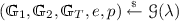
(Computational Security). We define two flavors for computational security notions: selectively and co-selectively secure master-key hiding ($\mathsf {SMH},\mathsf {CMH}$) in a bilinear group generator $\mathcal {G}$. We first define the following game template, denoted as $\mathsf {Exp}_{\mathcal {G}, \mathsf {P}, \mathsf {G},b,\mathcal {A},t_1,t_2}(\lambda )$, for pair encoding $\mathsf {P}$, a flavor $\mathsf {G}\in \{\mathsf {CMH},\mathsf {SMH}\}$, $b\in \{0,1\}$, and $t_1,t_2 \in \mathbb {N}$. It takes as input the security parameter $\lambda$ and does the experiment with the adversary $\mathcal {A}=(\mathcal {A}_1,\mathcal {A}_2)$, and outputs $b'$ (as a guess of b). Denote by $\mathsf {st}$ a state information by $\mathcal {A}$. The game is defined as:

where each oracle $\mathcal {O}^1,\mathcal {O}^2$ can be queried at most $t_1,t_2$ times respectively, and is defined as follows.

• Selective Security

  • – $\mathcal {O}^1_{\mathsf {\mathsf {SMH}},b,\alpha ,{\varvec{h}}}(Y)$: Run ; return ${\varvec{U}} \leftarrow g_1^{{\varvec{c}}({\varvec{s}},{\varvec{h}})}$.

  • – $\mathcal {O}^2_{\mathsf {\mathsf {SMH}},b,\alpha ,{\varvec{h}}}(X)$: If $R(X,Y)=1$ for some queried Y, then return $\bot$.

    Else, run ; return ${\varvec{V}} \leftarrow g_2^{{\varvec{k}}(b\alpha , {\varvec{r}},{\varvec{h}})}$.

• Co-selective Security

  • – $\mathcal {O}^1_{\mathsf {\mathsf {CMH}},b,\alpha ,{\varvec{h}}}(X)$: Run ; return ${\varvec{V}} \leftarrow g_2^{{\varvec{k}}(b \alpha , {\varvec{r}},{\varvec{h}})}$.

  • – $\mathcal {O}^2_{\mathsf {\mathsf {CMH}},b,\alpha ,{\varvec{h}}}(Y)$: If $R(X,Y)=1$ for some queried X, then return $\bot$.

    Else, run ; return ${\varvec{U}} \leftarrow g_1^{{\varvec{c}}({\varvec{s}},{\varvec{h}})}$.

We define the advantage of $\mathcal {A}$ against the pair encoding scheme $\mathsf {P}$ in the security game $\mathsf {G}\in \{\mathsf {SMH},\mathsf {CMH}\}$ for bilinear group generator $\mathcal {G}$ with the bounded number of queries $(t_1,t_2)$ as

$$\begin{aligned} \mathsf {Adv}_{\mathcal {A}}^{(t_1,t_2)\text {-}\mathsf {G}(\mathsf {P})}(\lambda ):= |\Pr [\mathsf {Exp}_{\mathcal {G}, \mathsf {P},\mathsf {G},0,\mathcal {A},t_1,t_2}(\lambda ) =1] - \Pr [ \mathsf {Exp}_{\mathcal {G}, \mathsf {P},\mathsf {G},1,\mathcal {A},t_1,t_2}(\lambda ) =1]| \end{aligned}$$

We say that $\mathsf {P}$ is $(t_1,t_2)\text {-}$ selectively master-key hiding in $\mathcal {G}$ if $\mathsf {Adv}_{\mathcal {A}}^{(t_1,t_2)\text {-}\mathsf {\mathsf {SMH}}(\mathsf {P})}(\lambda )$ is negligible for all polynomial time attackers $\mathcal {A}$. Analogously, $\mathsf {P}$ is $(t_1,t_2)\text {-}$ co-selectively master-key hiding in $\mathcal {G}$ if $\mathsf {Adv}_{\mathcal {A}}^{(t_1,t_2)\text {-}\mathsf {\mathsf {CMH}}(\mathsf {P})}(\lambda )$ is negligible for all polynomial time attackers $\mathcal {A}$.

Poly-many Queries. We also consider the case where $t_i$ is not a-priori bounded and hence the corresponding oracle can be queried polynomially many times. In such a case, we denote $t_i$ as $\textsf {poly}$.

Remark 2

The original notions considered in [3] are $(1,\textsf {poly})\text {-}\mathsf {SMH}$, $(1,1)\text {-}\mathsf {CMH}$ for selective and co-selective master-key hiding security, respectively. The refinement with $(t_1,t_2)$ is done recently in [10]. An advantage of this refinement is that we can have a “dual” conversion that converts between (1, 1)-$\mathsf {CMH}$ and (1, 1)-$\mathsf {SMH}$ for dual predicate [10].

Remark 3

The definition of computational security for encoding here is slightly different from that in [3, 10] in that here we define it in asymmetric and prime-order groups, while it was defined in symmetric and prime-order subgroup of composite-order groups in [3, 10]. We use asymmetric groups for the purpose of generality, one can obtain schemes in symmetric groups by just setting $\mathbb {G}_1=\mathbb {G}_2$. Hence, we can use all the proposed encodings in [3, 10] by working on the symmetric group version of our framework. For the latter issue, the difference of definitions between prime-order groups and prime-order subgroups are merely syntactic. This is since although the original definition was defined in prime-order subgroups, the hardness of factorization was not assumed (i.e., generators of each subgroup or even factors of composites N can be given out to the adversary). Hence, the encoding schemes in [3, 10] are secure in our definition under the security proofs in their present forms.

4 Approach for Translation to Prime-Order Groups

Before describing our prime-order framework, we intuitively describe how we translate elements, procedures, and properties from the composite-order group setting to the prime-order group setting, following the intuition overview in Sect. 1.3.

$\bullet$ Generators. In composite-order groups $({\mathbb {C}}_1,{\mathbb {C}}_2,{\mathbb {C}}_T)$ of order $N=p_1p_2p_3$, we consider generators $c_1 \in {\mathbb {C}}_{1,p_1}$, $\hat{c}_1 \in {\mathbb {C}}_{1,p_2}$, $c_2 \in {\mathbb {C}}_{2,p_1}$, $\hat{c}_2 \in {\mathbb {C}}_{2,p_2}$, where ${\mathbb {C}}_{i,p_j}$ is the subgroup of ${\mathbb {C}}_i$ of order $p_j$. In prime-order groups $(\mathbb {G}_1,\mathbb {G}_2,\mathbb {G}_T)$ with generators $g_1\in \mathbb {G}_1, g_2\in \mathbb {G}_2$, we use the following elements to mimic generators $c_1, \hat{c}_1, c_2, \hat{c}_2$, respectively:

where we let where the distribution $\mathcal {S}_d$ does as follows: sample , and set ${{\varvec{Z}}}:={{{\varvec{B}}}}^{-\top }{{\varvec{D}}}$ where .

$\bullet$ Variables. The role of parameter $h_k$ (in ${\varvec{h}}$) in the composite-order setting will be played by a matrix ${{\varvec{H}}}_k\in \mathbb {Z}_p^{(d+1) \times (d+1)}$. The role of randomness $s_j,r_j$ (in ${\varvec{s}},{\varvec{r}}$) to be exponentiated over $c_1,c_2$ in the composite-order setting for a ciphertext and a key will be played by vectors ${\varvec{s}}_j,{\varvec{r}}_j \in \mathbb {Z}_p^{d \times 1}$, respectively, in the prime-order setting. The role of randomness $\hat{s}_j,\hat{r}_j$ (in ${\varvec{{\hat{s}}}},{\varvec{{\hat{r}}}}$) to be exponentiated over $\hat{c}_1,\hat{c}_2$ will be used as it is (a scalar in $\mathbb {Z}_p$) in the prime-order setting.

$\bullet$ Exponentiation by parameter. To mimic exponentiation $c_1^{h_k}$, $\hat{c}_1^{\hat{h}_k}$, $c_2^{h_k}$, $\hat{c}_2^{\hat{h}_k}$ in the composite-order setting, we do the following in the prime-order setting:

$\bullet$ Exponentiation by randomness. To mimic exponentiation $c_1^{s_j}$, $\hat{c}_1^{\hat{s}_j}$, $c_2^{r_j}$, $\hat{c}_2^{\hat{r}_j}$, in the composite-order setting, we do the following in the prime-order setting:

$\bullet$ Exponentiation by randomness over parameter. To mimic $(c_1^{h_k})^{s_j}$, $(\hat{c}_1^{\hat{h}_k})^{\hat{s}_j}$, $(c_2^{h_k})^{r_j}$, $(\hat{c}_2^{\hat{h}_k})^{\hat{r}_j}$, in the composite-order setting, we do as follows:

$\bullet$ Evaluating Pair Encoding with Vectors/Matrices. We can evaluate the ciphertext attribute encoding ${\varvec{c}}({\varvec{s}},{\varvec{h}})$, defined in Eq.(5), with each $s_j$ being substituted by a vector ${\varvec{x}}_j \in \mathbb {Z}_p^{(d+1)\times 1}$ and each $h_k$ being substituted by a matrix ${{\varvec{H}}}_k \in \mathbb {Z}_p^{(d+1)\times (d+1)}$. Let ${{\varvec{X}}}=({\varvec{x}}_0,\ldots ,{\varvec{x}}_{w_2})\in \mathbb {Z}_p^{(d+1)\times (w_2+1)}$ and $\mathbb {H}=({{\varvec{H}}}_1,\ldots ,{{\varvec{H}}}_n)$. We define

$$\begin{aligned} {\varvec{c}}({{\varvec{X}}}, {{\varvec{\mathbb {H}}}} ):= \left\{ \left( \sum _{j\in [0,w_2]} a_{i,j} {\varvec{x}}_j \right) + \left( \sum _{\begin{array}{c} j\in [0,w_2] \\ k\in [1,n] \end{array}} a_{i,j,k} {{\varvec{H}}}_k {\varvec{x}}_j \right) \right\} _{i\in [1,w_1]}. \end{aligned}$$

(6)

Similarly for the key attribute encoding ${\varvec{k}}(\alpha ,{\varvec{r}},{\varvec{h}})$, defined in Eq. (4), we replace each $r_j$ with a vector ${\varvec{y}}_j \in \mathbb {Z}_p^{(d+1)\times 1}$ and $\alpha$ with ${\varvec{\alpha }}\in \mathbb {Z}_p^{(d+1)\times 1}$. Let ${{\varvec{Y}}}=({\varvec{y}}_1,\ldots ,{\varvec{y}}_{m_2})\in \mathbb {Z}_p^{(d+1)\times m_2}$. We define

$$\begin{aligned} {\varvec{k}}({\varvec{\alpha }}, {{\varvec{Y}}}, {{\varvec{\mathbb {H}}}} ):= \left\{ b_i {\varvec{\alpha }} + \left( \sum _{j\in [1,m_2]} b_{i,j} {\varvec{y}}_j \right) + \left( \sum _{\begin{array}{c} j\in [1,m_2] \\ k\in [1,n] \end{array}} b_{i,j,k} {{\varvec{H}}}_k^\top {\varvec{y}}_j \right) \right\} _{i\in [1,m_1]}. \end{aligned}$$

(7)

$\bullet$ Associativity. In the composite-order setting, we have that $e(t_1^{h_ks_j},t_2^{r_{i}}) = e(t_1^{s_j},t_2^{h_kr_{i}})$, for any $t_1\in {\mathbb {C}}_1, t_2\in {\mathbb {C}}_2$. In the prime-order setting, we have

(8)

as .

$\bullet$ Unavailable Commutativity. We also give an intuition why commutativity does not preserve to prime-order settings. In the composite-order setting, we allow for any $t_1\in {\mathbb {C}}_1, t_2\in {\mathbb {C}}_2$, $e(t_1^{h_ks_j},t_2^{h_{k'}r_{i}}) = e(t_1^{h_{k'}s_j},t_2^{h_kr_{i}})$. However, when translating to our prime-order setting using our rules so far, an analogous mechanism would not hold as we can see that:

(9)

as , due to the fact that the matrix multiplication is not commutative. This is exactly why we will not use this commutativity-based computation in our framework by disallowing exactly this kind of multiplication to occur. We enable this with the first rule of regular encoding, which exactly prevents multiplying $h_{k} s_{j}$ with $h_{k'} r_{j'}$.

$\bullet$ Parameter-Hiding. In composite-order groups, we have that: given $c_1^{h_k}, c_2^{h_k}, c_1, \hat{c}_1,c_2,\hat{c}_2, p_1,p_2$; $h_k \bmod p_2$ is information-theoretically hidden (due to the Chinese Remainder Theorem). In prime-order settings, we have Lemma 1.

Lemma 1

Let . For any ${{\varvec{H}}}_k \in \mathbb {Z}_p^{(d+1)\times (d+1)}$, we have that, given and , along with ${{\varvec{B}}}, {{\varvec{Z}}}$, the quantity of the entry at $(d+1,d+1)$ of the matrix ${{\varvec{B}}}^{-1}{{\varvec{H}}}_k{{\varvec{B}}}$ is information-theoretically hidden.

Proof

Write where $M_1\in \mathbb {Z}_p^{d \times d}$, $M_2\in \mathbb {Z}_p^{d \times 1}$, $M_3\in \mathbb {Z}_p^{1 \times d}$, and $\delta \in \mathbb {Z}_p$. We have

where in the second line, we use the fact that . We can see that both do not contain information on $\delta$.    $\square$

$\bullet$ Using Security of Encodings in Hybrid Games. In the composite-order setting, intuitively, we embed the security of encodings as it is in one hybrid game in the proof of the scheme. That is, we simply invoke a trivial implication:

$$\begin{aligned} \hat{c}_2^{{\varvec{k}}(0,\hat{{\varvec{r}}},\hat{{\varvec{h}}})} \approx _c \hat{c}_2^{{\varvec{k}}(\hat{\alpha },\hat{{\varvec{r}}},\hat{{\varvec{h}}})} \quad \Longrightarrow \quad \hat{c}_2^{{\varvec{k}}(0,\hat{{\varvec{r}}},\hat{{\varvec{h}}})} \approx _c \hat{c}_2^{{\varvec{k}}(\hat{\alpha },\hat{{\varvec{r}}},\hat{{\varvec{h}}})} \end{aligned}$$

where we refer the left-hand side as the security of encoding and the right-hand side as the hybrid in the proof of the scheme. Also, $\approx _c$ denotes computational indistinguishability (informally). In the prime-order setting, contrastingly, we will need to prove the following reduction: (stated informally here)

$$\begin{aligned} g_2^{{\varvec{k}}(0,\hat{{\varvec{r}}},\hat{{\varvec{h}}})} \approx _c g_2^{{\varvec{k}}(\hat{\alpha },\hat{{\varvec{r}}},\hat{{\varvec{h}}})} \quad \Longrightarrow \quad g_2^{{\varvec{k}}({\varvec{0}},{{\varvec{Z}}}\hat{{{\varvec{R}}}},\mathbb {H})}\approx _c g_2^{{\varvec{k}}(\hat{{\varvec{\alpha }}},{{\varvec{Z}}}\hat{{{\varvec{R}}}},\mathbb {H})} \end{aligned}$$

where the left-hand side refers to the same security of encodings as before, so that we can achieve our goal of using security of encoding “as is”.⁷ Now, however, the right-hand side, which refers to one hybrid in our scheme⁸, is of a different form, as it contains the matrix-based definition of encodings in Eq. (7). To this end, we will relate both sides as follows. First, we implicitly define $\hat{{\varvec{\alpha }}}$ from $\hat{\alpha }$, and $\hat{{{\varvec{R}}}}$ from $\hat{{\varvec{r}}}$.⁹ Second, we invoke the parameter-hiding property to implicitly replace each ${{\varvec{H}}}_k$ with in $\mathbb {H}$. Our novelty here then lies in identifying the following sufficient condition: (stated informally here)

where $\hat{\alpha }, \hat{{\varvec{r}}}=(\hat{r}_1,\ldots ,\hat{r}_{m_2}), \hat{{\varvec{h}}}=(\hat{h}_1,\ldots ,\hat{h}_{n})$ are unknown, and $b_{i,j,k}$ is defined by the encoding (Eq.(4)). We note that this is quite surprising in the first place, since we might expect that only $g_2^{{\varvec{k}}(\hat{\alpha },\hat{{\varvec{r}}},\hat{{\varvec{h}}})}$ would suffice to simulate $g_2^{{\varvec{k}}(\hat{{\varvec{\alpha }}},{{\varvec{Z}}}\hat{{{\varvec{R}}}},\mathbb {H})}$ (intuitively due to one-to-one translation of elements into matrix forms). Now, to establish the reduction, we require the availability of the latter term $(g_2^{\hat{r}_j})^{b_{i,j,k}}$, which was not a-priori guaranteed. We simply resolve this by observing that it is only available if either $\hat{r}_j$ is given out in the definition of ${\varvec{k}}(\hat{\alpha },\hat{{\varvec{r}}},\hat{{\varvec{h}}})$ or $b_{i,j,k}=0$. This is why we thus define this to be exactly one of the rules for regular encodings (Rule 2 of Definition 1). The case for the encoding ${\varvec{c}}$ can be argued analogously.

5 Our Generic Construction for Fully Secure ABE

We are now ready to describe our generic construction in prime-order groups. It is obtained by translating the composite-order scheme of [3], recapped also in the full version [4], to the prime-order setting using the above rules of Sect. 4.

We use the distribution $\mathcal {S}_d$ defined in Sect. 4. From a pair encoding scheme $\mathsf {P}$ for a predicate R, we construct an ABE scheme for R, denoted $\mathsf {ABE}(\mathsf {P})$, as follows.

• $\mathsf {Setup}(1^\lambda , \kappa )$: Run . Pick generators and . Run $n\leftarrow \mathsf {Param}(\kappa )$. Pick and . Sample . Note that ${{\varvec{B}}},{{\varvec{Z}}} \in \mathbb {Z}_p^{(d+1)\times (d+1)}$. Output

  

  (10)

• $\mathsf {Encrypt}(Y, {M}, \mathsf {PK})$: Upon input $Y\in \mathbb {Y}$, run $({\varvec{c}};w_2)\leftarrow \mathsf {Enc2}(Y)$. Randomly pick . Let . Output the ciphertext as ${\mathsf {CT}}=({\varvec{C}},C_0)$:

  

  (11)

• $\mathsf {KeyGen}(X, \mathsf {MSK})$: Upon input $X\in \mathbb {X}$, run $({\varvec{k}};m_2)\leftarrow \mathsf {Enc1}(X)$. Randomly pick . Let . Output

  

  (12)

• $\mathsf {Decrypt}({\mathsf {CT}},{\mathsf {SK}})$: Obtain Y, X from ${\mathsf {CT}},{\mathsf {SK}}$. Suppose $R(X,Y)=1$. Run ${{\varvec{E}}}\leftarrow \mathsf {Pair}(X,Y)$. Compute the mask

  

  (13)

  where we denote by ${\varvec{C}}[j] \in \mathbb {G}_1^{(d+1)\times 1}$ the j-th vector in ${\varvec{C}}$, and $\mathsf {SK}[i] \in \mathbb {G}_2^{(d+1)\times 1}$ the i-th vector in $\mathsf {SK}$. Finally, remove this mask from $C_0$ to get ${M}$.

Remark on Computability. We note that ${\varvec{C}}$ can be computed from $\mathsf {PK}$ since

(14)

and thanks to the identity relation for any ${{\varvec{X}}} \in \mathbb {Z}_p^{(d+1) \times (d+1)}$, ${\varvec{y}} \in \mathbb {Z}_p^{d \times 1}$. Similarly, $\mathsf {SK}$ can be computed from $\mathsf {MSK}$ since

(15)

Correctness. We would like to prove that if $R(X,Y)=1$ then

This is implied from the correctness of the pair encoding which states that: if $R(X,Y)=1$, then $\alpha s_0 = \sum _{\begin{array}{c} i\in [1,m_1], j\in [1,w_1] \end{array}} E_{i,j} \cdot {\varvec{k}}(\alpha ,{\varvec{r}},{\varvec{h}})[i] \cdot {\varvec{c}}({\varvec{s}},{\varvec{h}})[j]$. Intuitively, since we translate to the prime-order setting by substituting variables and procedures while preserving their properties as in Sect. 4, this relation should also translate to the above equation. In particular, we use associativity but not use commutativity, as clarified in Sect. 4. We verify the correctness more formally in the full version [4].

6 Security Theorems and Proofs

We obtain three security theorems for the generic construction. The first one is the main theorem and is for the case when the pair encoding is $(1,\mathsf {poly})$-$\mathsf {SMH}$ and (1, 1)-$\mathsf {CMH}$, where we achieve tighter reduction cost, $O(q_1)$. The other two are for the case of $\mathsf {PMH}$ and the pair of (1, 1)-$\mathsf {SMH}$, (1, 1)-$\mathsf {CMH}$, where we obtain normal reduction cost, $O(q_{ all })$. We postpone the latter two to [4].

Theorem 1

Suppose that a pair encoding scheme $\mathsf {P}$ for predicate R is $(1,\mathsf {poly})$-selectively and (1, 1)-co-selectively master-key hiding in $\mathcal {G}$, and the Matrix-DH Assumption holds in $\mathcal {G}$. Then the construction $\mathsf {ABE}(\mathsf {P})$ in $\mathcal {G}$ is fully secure. More precisely, for any PPT adversary $\mathcal {A}$, let $q_1$ denote the number of queries in phase 1, there exist PPT algorithms $\mathcal {B}_1,\mathcal {B}_2,\mathcal {B}_3$, whose running times are the same as $\mathcal {A}$ plus some polynomial times, such that for any $\lambda$,

$$\begin{aligned} \mathsf {Adv}_\mathcal {A}^{\mathsf {ABE}}(\lambda ) \le (2q_1+3) \mathsf {Adv}_{\mathcal {B}_1}^{\mathcal {D}_d\text {-}\mathsf {Mat}\mathsf {DH}}(\lambda ) + q_1\mathsf {Adv}_{\mathcal {B}_2}^{(1,1)\text {-}\mathsf {CMH}}(\lambda ) + \mathsf {Adv}_{\mathcal {B}_3}^{(1,\mathsf {poly})\text {-}\mathsf {SMH}}(\lambda ). \end{aligned}$$

Semi-functional Algorithms. We define semi-functional algorithms which will be used in the security proof. These are also translated from semi-functional algorithms from the framework of [3] (also recapped in [4]).

• $\mathsf {SFSetup}(1^\lambda , \kappa ) \rightarrow (\mathsf {PK}, \mathsf {MSK}, \widehat{\mathsf {PK}}, \widehat{\mathsf {MSK}}_{\mathsf {base}},\widehat{\mathsf {MSK}}_{\mathsf {aux}}):$ This is exactly the same as Setup albeit it additionally outputs also $\widehat{\mathsf {PK}}$, $\widehat{\mathsf {MSK}}_{\mathsf {base}}$, $\widehat{\mathsf {MSK}}_{\mathsf {aux}}$ defined as

  

  (16)
  

  (17)

• $\mathsf {SFEncrypt}(Y, {M}, \mathsf {PK}, \widehat{\mathsf {PK}}) \rightarrow {\mathsf {CT}}$: Run $({\varvec{c}};w_2)\leftarrow \mathsf {Enc2}(Y)$. Pick ${{\varvec{S}}}$ as in $\mathsf {Encrypt}$. Pick . Let $\hat{{{\varvec{S}}}} :=\left( \left( {\begin{matrix} {\varvec{0}} \\ {\hat{s}}_{0} \end{matrix}} \right) , \left( {\begin{matrix} {\varvec{0}} \\ {\hat{s}}_{1} \end{matrix}} \right) , \ldots , \left( {\begin{matrix} {\varvec{0}} \\ {\hat{s}}_{w_2} \end{matrix}} \right) \right) \in \mathbb {Z}_p^{(d+1) \times (w_2+1)}$. Output the ciphertext as ${\mathsf {CT}}=({\varvec{C}},C_0)$:

  

  (18)

• $\mathsf {SFKeyGen}(X, \mathsf {MSK}, \widehat{\mathsf {MSK}}_{\mathsf {base}}, \widehat{\mathsf {MSK}}_{\mathsf {aux}}, \mathsf {t}\in \{\mathsf {0}, \mathsf {1},\mathsf {2},\mathsf {3}\}, \beta \in \mathbb {Z}_p \big ) \rightarrow \mathsf {SK}$: Run $({\varvec{k}};m_2)\leftarrow \mathsf {Enc1}(X)$. Pick ${{\varvec{R}}}$ as in $\mathsf {KeyGen}$. Pick . $\hat{{{\varvec{R}}}}:=\left( \left( {\begin{matrix} {\varvec{0}} \\ {\hat{r}}_{1} \end{matrix}} \right) , \ldots , \left( {\begin{matrix} {\varvec{0}} \\ {\hat{r}}_{m_2} \end{matrix}} \right) \right) \in \mathbb {Z}_p^{(d+1) \times m_2}$ Output the secret key ${\mathsf {SK}}$:

  

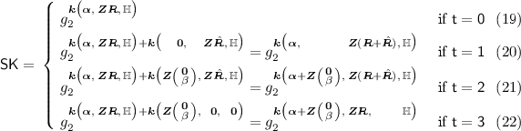
  We call $\mathsf {t}$ the type of semi-functional keys. Note that

  • – In computing type 0, 3, $\widehat{\mathsf {MSK}}_{\mathsf {aux}}$ is not required as input (and no $\hat{{{\varvec{R}}}}$ needed).

  • – In computing type 0, 1, $\beta$ is not required as input.

Proof (of Theorem 1)

We use a sequence of games in the following order:

where each game is defined as follows.¹⁰ $\mathsf {G}_{\text {real}}$ is the actual security game. Each of the following game is defined exactly as its previous game in the sequence except the specified modification as follows. For notational purpose, let $\mathsf {G}_{0,3}:=\mathsf {G}_0$.

• $\mathsf {G}_{0}$: We modify the challenge ciphertext to be semi-functional type.

• $\mathsf {G}_{i,t}$ where $i\in [1,q_1]$, $t\in \{1,2,3\}$: We modify the i-th queried key to be semi-functional of type-t. We use fresh $\beta$ for each key (for type $t=2,3$).

• $\mathsf {G}_{q_1+t}$ where $t\in \{1,2,3\}$: We modify all keys in phase 2 to be semi-functional of type-t at once. We use the same $\beta$ for all these keys (for type $t=2,3$).

• $\mathsf {G}_{ final }$: We modify the challenge to encrypt a random message.

In the final game, the advantage of $\mathcal {A}$ is trivially 0. We prove the indistinguishability between all these adjacent games (under the underlying assumptions as written in the diagram). Due to the lack of space, we defer most of them to [4] and show only the proof of the indistinguishability between $\mathsf {G}_ real$ and $\mathsf {G}_0$ under $\mathsf {MatDH}$ here below (Lemma 2). Other $\mathsf {MatDH}$-based transitions can be done similarly. On the other hand, the transitions based on the security of encodings (namely, $\mathsf {CMH}$ and $\mathsf {SMH}$), although are a bit more involved, will basically follow the intuition explained at the end of Sect. 4. In particular, we will be able to establish the reduction to the security of encodings thanks to the restriction for regular encodings (Rule 2–4) and the parameter-hiding lemma. From these, we obtain Theorem 1.   $\square$

Lemma 2

( $\mathsf {G}_{ real }$ to $\mathsf {G}_{0}$ ). For any adversary $\mathcal {A}$ against $\mathsf {ABE}$, there exists an algorithm $\mathcal {B}$ that breaks the $\mathcal {D}_d$-Matrix-DH with $|\mathsf {G}_{ real }\mathsf {Adv}_\mathcal {A}^{\mathsf {ABE}}(\lambda )- \mathsf {G}_{0}\mathsf {Adv}_\mathcal {A}^{\mathsf {ABE}}(\lambda )| \le \mathsf {Adv}_\mathcal {B}^{\mathcal {D}_d\text {-}\mathsf {Mat}\mathsf {DH}}(\lambda )$. (Denote $\mathsf {G}_{j}\mathsf {Adv}_\mathcal {A}^{\mathsf {ABE}}(\lambda )$ as the advantage of $\mathcal {A}$ in the game $\mathsf {G}_j$.)

Proof

(of Lemma  2 ). $\mathcal {B}$ obtains an input from the $\mathcal {D}_d$-Matrix DH Assumption where either , and , .

Setup. $\mathcal {B}$ runs $\mathsf {Setup}$ except that it uses $\mathbb {G}$ from its input, and that it will set $({{\varvec{B}}},{{\varvec{Z}}})$ in an implicit manner as follows. $\mathcal {B}$ chooses , and sets

where we recall that from Eq. (1). We can see that $({{\varvec{B}}},{{\varvec{Z}}})$ are properly distributed as from $\mathcal {S}_d$ as follows.

• ${{\varvec{B}}}$ is properly distributed due to uniformly random $\tilde{{{\varvec{B}}}}, {{\varvec{T}}} \in {\mathbb {GL}}_{p,d+1}$.

• ${{\varvec{Z}}}$ is properly distributed as we observe that ${{\varvec{D}}} ={{\varvec{B}}}^\top {{\varvec{Z}}}$ is

  

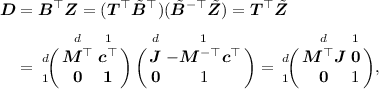
  where the last equality holds since $({{\varvec{M}}}^\top )(-{{\varvec{M}}}^{-\top }{\varvec{c}}^\top )+ ({\varvec{c}}^\top )(1) = {\varvec{0}}$ (for the upper right block). We can see that ${{\varvec{D}}}$ is properly distributed due to uniformly random ${{\varvec{M}}}^\top , {{\varvec{J}}} \in {\mathbb {GL}}_{p,d}$.

$\mathcal {B}$ can then compute $g_1^{{\varvec{B}}} = g_1^{\tilde{{{\varvec{B}}}} {{\varvec{T}}}}$ and . Here, the first term is computable from $g_1^{{\varvec{T}}}$, while in the second term, the unknown last column of ${{\varvec{Z}}}$ vanishes through the left projection map, . From these two terms, $\mathcal {B}$ can compute $\mathsf {PK},\mathsf {MSK}$. The public key $\mathsf {PK}$ is given to $\mathcal {A}$.

Phase 1, 2. $\mathcal {B}$ answer all key queries to $\mathcal {A}$ using $\mathsf {KeyGen}$ (with the known $\mathsf {MSK}$).

Challenge. The adversary $\mathcal {A}$ outputs ${M}_0,{M}_1 \in \mathbb {G}_T$ and a target $Y^\star$. $\mathcal {B}$ runs $({\varvec{c}};w_2)\leftarrow \mathsf {Enc2}(Y^\star )$ as usual. Using random self reducibility, $\mathcal {B}$ extends the Matrix-DH Assumption to $(w_2+1)$-fold and obtains where either ${\varvec{\hat{y}}}={\varvec{0}}$ or with , . $\mathcal {B}$ chooses and uses to compute ${\mathsf {CT}}^\star =({\varvec{C}}^\star ,C_0^\star )$ as

where we let be the first column of . This can be done since $\mathcal {B}$ possesses ${\varvec{\alpha }}, {{\varvec{\mathbb {H}}}} , \tilde{{{\varvec{B}}}}$. From this setting, we have

• If ${\varvec{\hat{y}}}={\varvec{0}}$, then ${\mathsf {CT}}^\star$ is exactly a normal ciphertext as in Eq. (11) with .

• If , then ${\mathsf {CT}}^\star$ is semi-functional as in Eq. (18) with .

Guess. The algorithm $\mathcal {B}$ has properly simulated $\mathsf {G}_{\text {real}}$ if $\hat{y}=0$ and $\mathsf {G}_{0}$ if . Hence, $\mathcal {B}$ can use the output of $\mathcal {A}$ to break the Matrix DH Assumption.    $\square$

7 Concrete Predicates and Our New Instantiations

In this section, we briefly describe the definitions of considering predicates and our new instantiations for them. Regarding the instantiations, their specifications are completely defined in Table 4, where we provide what pair encoding scheme to be instantiated for each scheme.

Dual, Conjunctive, and Dual-policy. We first define basic operations on predicates. For a predicate $R: \mathbb {X}\times \mathbb {Y}\rightarrow \{0,1\}$, its dual predicate is defined by $\bar{R}: \bar{\mathbb {X}}\times \bar{\mathbb {Y}}\rightarrow \{0,1\}$ where $\bar{\mathbb {X}}=\mathbb {Y}, \bar{\mathbb {Y}}=\mathbb {X}$ and $\bar{R}(X,Y):=R(Y,X)$. Let $R_1:\mathbb {X}_1\times \mathbb {Y}_1\rightarrow \{0,1\}$, $R_2:\mathbb {X}_2\times \mathbb {Y}_2\rightarrow \{0,1\}$ be two predicates. We define the conjunctive predicate of $R_1,R_2$ as $[R_1\wedge R_2]:\tilde{\mathbb {X}} \times \tilde{\mathbb {Y}}\rightarrow \{0,1\}$ where $\tilde{\mathbb {X}}=\mathbb {X}_1 \times \mathbb {X}_2$, $\tilde{\mathbb {Y}}=\mathbb {Y}_1 \times \mathbb {Y}_2$ and $[R_1\wedge R_2]((X_1,X_2),(Y_1,Y_2))=1$ iff $R_1(X_1,Y_1)=1$ and $R_2(X_2,Y_2)=1$. For predicate R, we define its dual-policy predicate (DP) [8, 10] as the conjunctive of itself and its dual predicate, $\bar{R}$. Generic dual and conjunctive conversions (and hence also dual-policy conversion) for pair encodings are recently given in [10]. We mostly use this conjunctive conversion to obtain dual-policy variants. It is indicated by ‘+’ in Table 4.

Table 4. Our instantiations

ABE for Policy over Doubly-Spatial Relation (ABE-PDS). This predicate was defined in [3] as a generalization that captures doubly-spatial encryption [23] and ABE for monotone span programs (and hence Boolean formulae) into one primitive. We refer the definition to [3]. By using exactly the same encodings as in [3, 10], we automatically obtain the first fully-secure prime-order KP-ABE-PDS, CP-ABE-PDS, DP-ABE-PDS schemes ($\mathbf{New }_{1}$-$\mathbf{New }_{3}$).

ABE for Monotone Span Programs (ABE-MSP). Let $\mathcal {U}$ be the universe of attributes. If $|\mathcal {U}|$ is of super-polynomial size, it is called large universe [21, 39], otherwise, it is small universe. In ABE-MSP [21], a policy is specified by a monotone span program $(A,\rho )$ where A is an integer matrix of dimension $m \times k$ for some m, k, and $\rho$ is a map $\rho :[1,m]\rightarrow \mathcal {U}$. For a set of attributes $S\subseteq \mathcal {U}$, let $A|_S$ be the sub-matrix of A that takes all the rows j such that $\rho (j)\in S$. We say that $(A,\rho )$ accepts S if $(1,0,\ldots ,0)\in rowspan (A|_S)$. ABE-MSP is the most popular predicate studied in the literature since it is known to imply ABE for Boolean formulae [21]. Let $t:=|S|$. Some schemes specifies bounds on maximum allowed sizes of t, m, k (we denote these bounds as T, M, K). Some may restrict the maximum number, denoted by R, of attribute multi-use in one policy (that is, the number of distinct i for the same $\rho (i)$). We call a large-universe scheme without any bounds a completely unbounded ABE scheme.

By using the same encodings as in [3, 10], we obtain the first fully-secure, prime-order ABE-MSP with various properties: completely unbounded KP/CP/DP-ABE, and short-ciphertext KP-ABE, short-key CP-ABE ($\mathbf{New }_{4}$-$\mathbf{New }_{8}$). By using encodings in [3] for bounded schemes, we also obtain some bounded schemes $\mathbf{New }'_{9}$-$\mathbf{New }_{14}$; these latter encodings are perfectly master-key hiding, hence the resulting schemes rely solely on the Matrix-DH assumption. Furthermore, we also observe that, by using also new encodings in [7] (which is then a subsequent work based on our work), we further obtain the first DP-ABE with short ciphertexts ($\mathbf{Newer }_{28}$), or short keys ($\mathbf{Newer }_{29}$).

For concreteness, we explicitly give the description for one of our instantiations, $\mathbf{New }_{4}$, in the full version [4].

Table 5. Performance by each KP-ABE for monotone span programs

Table 6. Performance by each CP-ABE for monotone span programs

Performances of Our ABE-MSP Schemes. We compare performances of our KP-ABE-MSP, CP-ABE-MSP to others in the literature in Tables 5 and 6, respectively. For clarity of comparison, we augment schemes in the literature which were proposed for one-use, to multi-use (with bound R) by using the transformation in [33]. Available pair encodings in [3, 10] were proved secure in symmetric groups, hence to be able to use them as they are, we will evaluate our construction at $d=2$, which yields the most efficient instantiations in symmetric settings. In such a case, schemes can rely on DLIN (See also Remark 5).

The numbers of group elements in our schemes for $\mathsf {SK},{\mathsf {CT}}$ are 3 times as large as their composite-order counterparts in A14, AY15 [3, 10]. But since composite-order elements are 12 times larger than prime-order ones [22], we achieve improvements of 25 % size reduction. More importantly, time performance is significantly improved. We recall that pairing is 250 times slower in composite-order groups than in prime-order ones [22]. In unbounded ABE ($\mathbf{New }_{4}$, $\mathbf{New }_{5}$), the dominant operation is pairing, and the numbers of pairings in decryption are 3 times as large as their composite-order counterparts in [3, 10]. As a result, our decryption is about 80 times faster. In constant-size ABE ($\mathbf{New }_{7}$, $\mathbf{New }_{8}$), the numbers of pairing are constant, and exponentiation may dominate (depending on m, T), but the improvement is similar, since exponentiation (in $\mathbb {G}_1,\mathbb {G}_2$) can be more than 200 times faster in prime-order groups [22, Table 6].

Remark 4

The underlying pair encodings of our schemes $\mathbf{New }_{4},\mathbf{New }_{7}$ are those proposed in [3, Sect. 7.1, 7.2], of which security rely on parameterized assumptions, namely, EDHE3, EDHE4, also given in [3]. We indeed use prime-order group versions, hence denoted as EDHE3p, EDHE4p, instead of prime-order subgroup in composite-order group as defined in [3]. These are defined exactly the same as the original except only that the group generator $\mathbb {G}$ outputs a prime-order group instead of a composite-order group (see [3, Defininition 6, 7]). For self-containment, we recapture them in the full version [4]. This modification is merely syntactic, see Remark 3.

Remark 5

As mentioned above, we use $d=2$ so that the security and assumptions for available pair encoding schemes can be argued in the present form. On the other hand, if we are willing to modify the assumptions and security proofs of pair encodings in [3, 10] to asymmetric groups, we can also instantiate at $d=1$, where we can rely on the SXDH assumption (for framework). This yields even more efficient construction.

The modification for assumptions (such as EDHE3p, EDHE4p) to asymmetric settings can be done straightforwardly by defining all elements in both groups $\mathbb {G}_1,\mathbb {G}_2$ (instead of $\mathbb {G}$ in symmetric settings). The proof can be modified by using $\mathbb {G}_1$ for all elements of ciphertexts, and $\mathbb {G}_2$ for all elements of keys, as defined in our construction. To optimize the size of assumptions (which is otherwise two times larger than the original), we can use automated tools of [1].

ABE for Regular Languages (ABE-RL). In ABE-RL [45], a policy is a deterministic finite automata (DFA) M, and an input to policy is a string w, and $R(M,w)=1$ if the automata M accepts the string w. We defer the detailed definition to [3, 4]. We obtain the first fully-secure prime-order KP-ABE, CP-ABE, DP-ABE for regular languages ($\mathbf{New }_{15}$-$\mathbf{New }_{17}$).

ABE for Branching Programs (ABE-BP). In ABE-BP [19], a policy is associated to a branching program $\varGamma$, which is a directed acyclic graph in which every non-terminal node has exactly two outgoing edges labeled (i, 0) and (i, 1) for some $i\in \mathbb {N}$. For an edge j, denote its label as $\ell _j$. Moreover, there is a distinguished terminal node called accept node. We can also assume wlog that there is exactly one start node. We can assume wlog that there is at most only one edge connecting any two nodes in $\varGamma$ (See [19]).

An input to policy is a binary string w. Every input binary string w induces a subgraph $\varGamma _w$ that contains exactly all the edges labeled $(i,w_i)$ for $i\in [1,|w|]$, where we write $w=(w_1,\ldots , w_{|w|})$ as the binary representation of w. We say that $\varGamma$ accepts w if there is a path from the start node to the accept node in $\varGamma _w$. If the allow length of w is bounded, we say that it is a bounded ABE-BP, otherwise, it is an unbounded scheme. In the latter, a label (i, b) has no bound on i.

We invoke the following theorem, which holds unconditionally.

Theorem 2

Large-universe ABE-MSP implies ABE-BP.

Remark 6

Karchmer and Wigderson proved in 1993 [26] that $\mathbf SL \subseteq \mathbf PSP$ (Symmetric Logspace $\subseteq$ Poly-size Span Program). Thus, the ABE-MSP-to-ABE-BP implication can be inferred from this. (We thank an anonymous reviewer for pointing this out.) Nevertheless, to the best of our knowledge, there is no explicit use of this theorem in the context of ABE, as ABE-MSP and ABE-BP were often studied separately. For self-containment and independent interest, we offer our alternative proof for this ABE-MSP-to-ABE-BP implication in the full version [4].

Our proof for this implication in [4] is constructive and the conversion preserves efficiency and the unbounded property (if satisfied) of the original ABE-MSP. Therefore, by using our instantiated ABE-MSP, we obtain the first schemes for the following schemes of ABE-BP: unbounded, short-ciphertext, short-key for all KP/CP/DP variants of ABE-BP (See Table 4). Our schemes are the first such schemes for each given property, not to mention that they are fully-secure and prime-order schemes. (This is with the only exception to the selectively-secure short-key KP-ABE-BP of [20]).

8 Generic Construction from Simpler Basis

Our main construction in Sect. 5 is based upon the original basis of PDSG in [15], where both ${{\varvec{B}}},{{\varvec{B}}}^{-\top }$ are required for setup. Chen et al. [14] proposed a simpler basis where the inverse matrix is not required. This substantially simplifies the proofs for subgroup decision-like assumptions provided by PDSG. In this section, we provide a simplification of our scheme using the basis from [14].

Simpler Basis from CGW [14]. Let $\mathcal {W}_d$ be an efficiently samplable distribution of pair $({{\varvec{A}}},{\varvec{a}}^\perp )$ over $\mathbb {Z}_p^{(d+1)\times d} \times \mathbb {Z}_p^{(d+1)\times 1}$ so that $({\varvec{a}}^\perp )^\top {{\varvec{A}}} ={\varvec{0}}$ and ${\varvec{a}}^\perp \ne {\varvec{0}}$. A useful property of $\mathcal {W}_d$ is the Basis Lemma [14], which we also recap in [4].

Our Simplified Construction. From a pair encoding scheme $\mathsf {P}$, our simplified generic construction, denoted $\mathsf {SimplerABE}(\mathsf {P})$, can be described as follows. The correctness, the security theorem, and the security proof are similar to our main construction and are deferred to [4].

• $\mathsf {Setup}(1^\lambda , \kappa )$: Run . Pick generators and . Run $n\leftarrow \mathsf {Param}(\kappa )$. Pick . Sample and . Choose . Output

  

  (23)

• $\mathsf {Encrypt}(Y, {M}, \mathsf {PK})$: Upon input $Y\in \mathbb {Y}$, run $({\varvec{c}};w_2)\leftarrow \mathsf {Enc2}(Y)$. Randomly pick . Output the ciphertext as ${\mathsf {CT}}=({\varvec{C}},C_0)$:

  

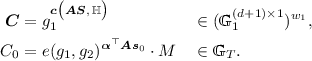  (24)

• $\mathsf {KeyGen}(X, \mathsf {MSK})$: Upon input $X\in \mathbb {X}$, run $({\varvec{k}};m_2)\leftarrow \mathsf {Enc1}(X)$. Randomly pick . Output

  

  (25)

• $\mathsf {Decrypt}({\mathsf {CT}},{\mathsf {SK}})$: Obtain Y, X from ${\mathsf {CT}},{\mathsf {SK}}$. Suppose $R(X,Y)=1$. Run ${{\varvec{E}}}\leftarrow \mathsf {Pair}(X,Y)$. Compute $e(g_1,g_2)^{{\varvec{\alpha }}^\top {{\varvec{A}}} {\varvec{s}}_0} = \prod _{\begin{array}{c} i\in [1,m_1], j\in [1,w_1] \end{array}} e({\varvec{C}}[j],\mathsf {SK}[i])^{E_{i,j}}.$ Finally, remove this mask from $C_0$ to get ${M}$.

References

Abe, M., Groth, J., Ohkubo, M., Tango, T.: Converting cryptographic schemes from symmetric to asymmetric bilinear groups. In: Garay, J.A., Gennaro, R. (eds.) CRYPTO 2014. LNCS, vol. 8616, pp. 241–260. Springer, Heidelberg (2014). doi:10.1007/978-3-662-44371-2_14
Agrawal, S., Chase, M.: A study of pair encodings: predicate encryption in prime order groups. In: Kushilevitz, E., Malkin, T. (eds.) TCC 2016. LNCS, vol. 9563, pp. 259–288. Springer, Heidelberg (2016). doi:10.1007/978-3-662-49099-0_10
Attrapadung, N.: Dual system encryption via doubly selective security: framework, fully secure functional encryption for regular languages, and more. In: Nguyen, P.Q., Oswald, E. (eds.) EUROCRYPT 2014. LNCS, vol. 8441, pp. 557–577. Springer, Heidelberg (2014). doi:10.1007/978-3-642-55220-5_31. Full version available at Cryptology ePrint Archive: Report 2014/428
Attrapadung, N.: Dual system encryption framework in prime-order groups via computational pair encodings. Full version of this paper. Cryptology ePrint Archive: Report 2015/390 (2015)
Attrapadung, N., Hanaoka, G., Matsumoto, T., Teruya, T., Yamada, S.: Attribute based encryption with direct efficiency tradeoff. In: Manulis, M., Sadeghi, A.-R., Schneider, S. (eds.) ACNS 2016. LNCS, vol. 9696, pp. 249–266. Springer, Heidelberg (2016). doi:10.1007/978-3-319-39555-5_14
Attrapadung, N., Hanaoka, G., Ogawa, K., Ohtake, G., Watanabe, H., Yamada, S.: Attribute-based encryption for range attributes. In: Zikas, V., Prisco, R. (eds.) SCN 2016. LNCS, vol. 9841, pp. 42–61. Springer, Heidelberg (2016). doi:10.1007/978-3-319-44618-9_3
Attrapadung, N., Hanaoka, G., Yamada, S.: Conversions among several classes of predicate encryption and applications to ABE with various compactness tradeoffs. In: Iwata, T., Cheon, J.H. (eds.) ASIACRYPT 2015. LNCS, vol. 9452, pp. 575–601. Springer, Heidelberg (2015). doi:10.1007/978-3-662-48797-6_24
Attrapadung, N., Imai, H.: Dual-policy attribute based encryption. In: Abdalla, M., Pointcheval, D., Fouque, P.-A., Vergnaud, D. (eds.) ACNS 2009. LNCS, vol. 5536, pp. 168–185. Springer, Heidelberg (2009). doi:10.1007/978-3-642-01957-9_11
Attrapadung, N., Libert, B., Panafieu, E.: Expressive key-policy attribute-based encryption with constant-size ciphertexts. In: Catalano, D., Fazio, N., Gennaro, R., Nicolosi, A. (eds.) PKC 2011. LNCS, vol. 6571, pp. 90–108. Springer, Heidelberg (2011). doi:10.1007/978-3-642-19379-8_6
Attrapadung, N., Yamada, S.: Duality in ABE: converting attribute based encryption for dual predicate and dual policy via computational encodings. In: Nyberg, K. (ed.) CT-RSA 2015. LNCS, vol. 9048, pp. 87–105. Springer, Heidelberg (2015). doi:10.1007/978-3-319-16715-2_5. Full version available at Cryptology ePrint Archive: Report 2015/157
Boneh, D., Gentry, C., Gorbunov, S., Halevi, S., Nikolaenko, V., Segev, G., Vaikuntanathan, V., Vinayagamurthy, D.: Fully key-homomorphic encryption, arithmetic circuit ABE and compact garbled circuits. In: Nguyen, P.Q., Oswald, E. (eds.) EUROCRYPT 2014. LNCS, vol. 8441, pp. 533–556. Springer, Heidelberg (2014). doi:10.1007/978-3-642-55220-5_30
Boneh, D., Sahai, A., Waters, B.: Functional encryption: definitions and challenges. In: Ishai, Y. (ed.) TCC 2011. LNCS, vol. 6597, pp. 253–273. Springer, Heidelberg (2011). doi:10.1007/978-3-642-19571-6_16
Chase, M., Meiklejohn, S.: Déjà Q: using dual systems to revisit q-type assumptions. In: Nguyen, P.Q., Oswald, E. (eds.) EUROCRYPT 2014. LNCS, vol. 8441, pp. 622–639. Springer, Heidelberg (2014). doi:10.1007/978-3-642-55220-5_34
Chen, J., Gay, R., Wee, H.: Improved dual system ABE in prime-order groups via predicate encodings. In: Oswald, E., Fischlin, M. (eds.) EUROCRYPT 2015. LNCS, vol. 9057, pp. 595–624. Springer, Heidelberg (2015). doi:10.1007/978-3-662-46803-6_20
Chen, J., Wee, H.: Fully, (Almost) tightly secure ibe and dual system groups. In: Canetti, R., Garay, J.A. (eds.) CRYPTO 2013. LNCS, vol. 8043, pp. 435–460. Springer, Heidelberg (2013). doi:10.1007/978-3-642-40084-1_25
Chen, J., Wee, H.: Semi-adaptive attribute-based encryption and improved delegation for boolean formula. In: Abdalla, M., Prisco, R. (eds.) SCN 2014. LNCS, vol. 8642, pp. 277–297. Springer, Heidelberg (2014). doi:10.1007/978-3-319-10879-7_16
Escala, A., Herold, G., Kiltz, E., Ràfols, C., Villar, J.: An algebraic framework for Diffie-Hellman assumptions. In: Canetti, R., Garay, J.A. (eds.) CRYPTO 2013. LNCS, vol. 8043, pp. 129–147. Springer, Heidelberg (2013). doi:10.1007/978-3-642-40084-1_8
Freeman, D.M.: Converting pairing-based cryptosystems from composite-order groups to prime-order groups. In: Gilbert, H. (ed.) EUROCRYPT 2010. LNCS, vol. 6110, pp. 44–61. Springer, Heidelberg (2010). doi:10.1007/978-3-642-13190-5_3
Gorbunov, S., Vaikuntanathan, V., Wee, H.: Attribute-based encryption for circuits. In: STOC 2013 (2013)
Gorbunov, S., Vinayagamurthy, D.: Riding on asymmetry: efficient ABE for branching programs. In: Iwata, T., Cheon, J.H. (eds.) ASIACRYPT 2015. LNCS, vol. 9452, pp. 550–574. Springer, Heidelberg (2015). doi:10.1007/978-3-662-48797-6_23
Goyal, V., Pandey, O., Sahai, A., Waters, B.: Attribute-based encryption for fine-grained access control of encrypted data. In: ACM CCS 2006, pp. 89–98 (2006)
Guillevic, A.: Comparing the pairing efficiency over composite-order and prime-order elliptic curves. In: Jacobson, M., Locasto, M., Mohassel, P., Safavi-Naini, R. (eds.) ACNS 2013. LNCS, vol. 7954, pp. 357–372. Springer, Heidelberg (2013). doi:10.1007/978-3-642-38980-1_22
Hamburg, M.: Spatial Encryption. Cryptology. ePrint Archive: Report 2011/389
Herold, G., Hesse, J., Hofheinz, D., Ràfols, C., Rupp, A.: Polynomial spaces: a new framework for composite-to-prime-order transformations. In: Garay, J.A., Gennaro, R. (eds.) CRYPTO 2014. LNCS, vol. 8616, pp. 261–279. Springer, Heidelberg (2014). doi:10.1007/978-3-662-44371-2_15
Ishai, Y., Wee, H.: Partial garbling schemes and their applications. In: Esparza, J., Fraigniaud, P., Husfeldt, T., Koutsoupias, E. (eds.) ICALP 2014. LNCS, vol. 8572, pp. 650–662. Springer, Heidelberg (2014). doi:10.1007/978-3-662-43948-7_54
Karchmer, M., Wigderson, A.: On span programs. In: Structure in Complexity Theory Conference (1993)
Kowalczyk, L., Lewko, A.B.: Bilinear entropy expansion from the decisional linear assumption. In: Gennaro, R., Robshaw, M. (eds.) CRYPTO 2015. LNCS, vol. 9216, pp. 524–541. Springer, Heidelberg (2015). doi:10.1007/978-3-662-48000-7_26. Report 2014/754 (retrieved version: Sep. 4, 2015)
Lewko, A.: Tools for simulating features of composite order bilinear groups in the prime order setting. In: Pointcheval, D., Johansson, T. (eds.) EUROCRYPT 2012. LNCS, vol. 7237, pp. 318–335. Springer, Heidelberg (2012). doi:10.1007/978-3-642-29011-4_20
Lewko, A., Meiklejohn, S.: A profitable sub-prime loan: obtaining the advantages of composite order in prime-order bilinear groups. In: Katz, J. (ed.) PKC 2015. LNCS, vol. 9020, pp. 377–398. Springer, Heidelberg (2015). doi:10.1007/978-3-662-46447-2_17
Lewko, A., Waters, B.: New techniques for dual system encryption and fully secure HIBE with short ciphertexts. In: Micciancio, D. (ed.) TCC 2010. LNCS, vol. 5978, pp. 455–479. Springer, Heidelberg (2010). doi:10.1007/978-3-642-11799-2_27
Lewko, A., Waters, B.: Unbounded HIBE and attribute-based encryption. In: Paterson, K.G. (ed.) EUROCRYPT 2011. LNCS, vol. 6632, pp. 547–567. Springer, Heidelberg (2011). doi:10.1007/978-3-642-20465-4_30
Lewko, A., Waters, B.: New proof methods for attribute-based encryption: achieving full security through selective techniques. In: Safavi-Naini, R., Canetti, R. (eds.) CRYPTO 2012. LNCS, vol. 7417, pp. 180–198. Springer, Heidelberg (2012). doi:10.1007/978-3-642-32009-5_12
Lewko, A., Okamoto, T., Sahai, A., Takashima, K., Waters, B.: Fully secure functional encryption: attribute-based encryption and (hierarchical) inner product encryption. In: Gilbert, H. (ed.) EUROCRYPT 2010. LNCS, vol. 6110, pp. 62–91. Springer, Heidelberg (2010). doi:10.1007/978-3-642-13190-5_4
Meiklejohn, S., Shacham, H., Freeman, D.M.: Limitations on transformations from composite-order to prime-order groups: the case of round-optimal blind signatures. In: Abe, M. (ed.) ASIACRYPT 2010. LNCS, vol. 6477, pp. 519–538. Springer, Heidelberg (2010). doi:10.1007/978-3-642-17373-8_30
Okamoto, T., Takashima, K.: Hierarchical predicate encryption for inner-products. In: Matsui, M. (ed.) ASIACRYPT 2009. LNCS, vol. 5912, pp. 214–231. Springer, Heidelberg (2009). doi:10.1007/978-3-642-10366-7_13
Okamoto, T., Takashima, K.: Fully secure functional encryption with general relations from the decisional linear assumption. In: Rabin, T. (ed.) CRYPTO 2010. LNCS, vol. 6223, pp. 191–208. Springer, Heidelberg (2010). doi:10.1007/978-3-642-14623-7_11
Okamoto, T., Takashima, K.: Fully secure unbounded inner-product and attribute-based encryption. In: Wang, X., Sako, K. (eds.) ASIACRYPT 2012. LNCS, vol. 7658, pp. 349–366. Springer, Heidelberg (2012). doi:10.1007/978-3-642-34961-4_22
Parno, B., Raykova, M., Vaikuntanathan, V.: How to delegate and verify in public: verifiable computation from attribute-based encryption. In: Cramer, R. (ed.) TCC 2012. LNCS, vol. 7194, pp. 422–439. Springer, Heidelberg (2012). doi:10.1007/978-3-642-28914-9_24
Rouselakis, Y., Waters, B..: Practical constructions and new proof methods for large universe attribute-based encryption. In: ACM CCS 2013, pp. 463–474 (2013)
Sahai, A., Waters, B.: Fuzzy identity-based encryption. In: Cramer, R. (ed.) EUROCRYPT 2005. LNCS, vol. 3494, pp. 457–473. Springer, Heidelberg (2005). doi:10.1007/11426639_27
Seo, J.H., Cheon, J.H.: Beyond the limitation of prime-order bilinear groups, and round optimal blind signatures. In: Cramer, R. (ed.) TCC 2012. LNCS, vol. 7194, pp. 133–150. Springer, Heidelberg (2012). doi:10.1007/978-3-642-28914-9_8
Takashima, K.: Expressive attribute-based encryption with constant-size ciphertexts from the decisional linear assumption. In: Abdalla, M., Prisco, R. (eds.) SCN 2014. LNCS, vol. 8642, pp. 298–317. Springer, Heidelberg (2014). doi:10.1007/978-3-319-10879-7_17
Waters, B.: Ciphertext-policy attribute-based encryption: an expressive, efficient, and provably secure realization. In: Catalano, D., Fazio, N., Gennaro, R., Nicolosi, A. (eds.) PKC 2011. LNCS, vol. 6571, pp. 53–70. Springer, Heidelberg (2011). doi:10.1007/978-3-642-19379-8_4
Waters, B.: Dual system encryption: realizing fully secure IBE and HIBE under simple assumptions. In: Halevi, S. (ed.) CRYPTO 2009. LNCS, vol. 5677, pp. 619–636. Springer, Heidelberg (2009). doi:10.1007/978-3-642-03356-8_36
Waters, B.: Functional encryption for regular languages. In: Safavi-Naini, R., Canetti, R. (eds.) CRYPTO 2012. LNCS, vol. 7417, pp. 218–235. Springer, Heidelberg (2012). doi:10.1007/978-3-642-32009-5_14
Wee, H.: Dual system encryption via predicate encodings. In: Lindell, Y. (ed.) TCC 2014. LNCS, vol. 8349, pp. 616–637. Springer, Heidelberg (2014). doi:10.1007/978-3-642-54242-8_26
Wee, H.: Déjà Q: encore! un petit IBE. In: Kushilevitz, E., Malkin, T. (eds.) TCC 2016. LNCS, vol. 9563, pp. 237–258. Springer, Heidelberg (2016). doi:10.1007/978-3-662-49099-0_9
Author information
Authors and Affiliations
Corresponding author
Editor information
Editors and Affiliations
Rights and permissions
Copyright information
© 2016 International Association for Cryptologic Research
About this paper
Cite this paper
Attrapadung, N. (2016). Dual System Encryption Framework in Prime-Order Groups via Computational Pair Encodings. In: Cheon, J., Takagi, T. (eds) Advances in Cryptology – ASIACRYPT 2016. ASIACRYPT 2016. Lecture Notes in Computer Science(), vol 10032. Springer, Berlin, Heidelberg. https://doi.org/10.1007/978-3-662-53890-6_20
Download citation
DOI: https://doi.org/10.1007/978-3-662-53890-6_20
Published:
Publisher Name: Springer, Berlin, Heidelberg
Print ISBN: 978-3-662-53889-0
Online ISBN: 978-3-662-53890-6
eBook Packages: Computer ScienceComputer Science (R0)