
Abstract
We present a multi-key fully homomorphic encryption scheme that supports an unbounded number of homomorphic operations for an unbounded number of parties. Namely, it allows to perform arbitrarily many computational steps on inputs encrypted by an a-priori unbounded (polynomial) number of parties. Inputs from new parties can be introduced into the computation dynamically, so the final set of parties needs not be known ahead of time. Furthermore, the length of the ciphertexts, as well as the space complexity of an atomic homomorphic operation, grow only linearly with the current number of parties.
Prior works either supported only an a-priori bounded number of parties (López-Alt, Tromer and Vaikuntanthan, STOC ’12), or only supported single-hop evaluation where all inputs need to be known before the computation starts (Clear and McGoldrick, Crypto ’15, Mukherjee and Wichs, Eurocrypt ’16). In all aforementioned works, the ciphertext length grew at least quadratically with the number of parties.
Technically, our starting point is the LWE-based approach of previous works. Our result is achieved via a careful use of Gentry’s bootstrapping technique, tailored to the specific scheme. Our hardness assumption is that the scheme of Mukherjee and Wichs is circular secure (and thus bootstrappable). A leveled scheme can be achieved under standard LWE.
Z. Brakerski—Supported by the Israel Science Foundation (Grant No. 468/14), the Alon Young Faculty Fellowship, Binational Science Foundation (Grant No. 712307) and Google Faculty Research Award.
R. Perlman—This work took place at the Weizmann Institute of Science as a part of the Young Weizmann Scholars program for outstanding undergraduate students.
You have full access to this open access chapter, Download conference paper PDF
Keywords
- Ciphertext
- Fully Homomorphic Encryption (FHE)
- Learning With Errors (LWE)
- Circular Security
- Evaluation Homomorphism
These keywords were added by machine and not by the authors. This process is experimental and the keywords may be updated as the learning algorithm improves.
1 Introduction
In 1978, Rivest et al. [RAD78] envisioned an encryption scheme where it is possible to publicly convert an encryption of a message x into an encryption of f(x) for any f, thus enabling private outsourcing of computation. It took over 30 years for the first realization of this so called fully homomorphic encryption (FHE) to materialize in Gentry’s breakthrough work [Gen09b, Gen09a], but since then progress has been consistent and rapid. López-Alt et al. [LTV12] considered an extension of this vision into the multi-key setting, where it is possible to compute on encrypted messages even if they were not encrypted using the same key. In multi-key FHE, a public evaluator takes ciphertexts encrypted under different keys, and evaluates arbitrary functions on them. The resulting ciphertext can then be decrypted using the collection of keys of all parties involved in the computation. Note that the security of the encryption scheme compels that all keys need to be used for decryption.
In the dream version of multi-key FHE, each user generates keys for itself and encrypts messages at will. Any third party can then perform an arbitrary computation on any set of encryptions by any set of users. The resulting ciphertext is attributed to the set of users whose ciphertexts were used to create it, and the collection of all of their secret keys is required in order to decrypt it. Most desirable is a fully dynamic setting where nothing at all about the parties needs to be known ahead of time: not their identities, not their number and not the order in which they will join the computation. In particular, outputs of previous evaluations can be used as inputs to new evaluations regardless of whether they correspond to the same set of users, intersecting sets or disjoint sets. In short, any operation can be performed on any ciphertext at any point in time, and of course while maintaining ciphertext compactness. However, as we explain below, existing solutions fall short of achieving this functionality.
Multi-key FHE can be useful in various situations involving multiple parties that do not coordinate ahead of time, but only after the fact. In [LTV12], the main motivation is performing on-the-fly multiparty computation (MPC) where various parties wish to use a cloud server (or some other untrusted third party) to perform some computation without revealing their private inputs and while having minimal interaction with the server. In this setting, the parties first send their encrypted input to the cloud, which performs the homomorphic operation and sends the output to the parties. The parties then execute a multiparty computation protocol for joint decryption. A similar approach was used by Mukherjee and Wichs [MW16] to construct a 2-round MPC protocol in the common random string setting. We note that one could also consider using this primitive in simpler situations, such as ones where the respective secret keys are being sold after the fact, and the owner of subset of keys can decrypt the output of the respective computation by himself.
As we mentioned, multi-key FHE was introduced by [LTV12] who also introduced the first candidate scheme, building upon the NTRU encryption scheme. Their candidate was almost fully dynamic, except an upper bound on the maximal number of participants in a computation had to be known at the time a key is generated. In particular, to support computation amongst N parties, the bit-length of a ciphertext in their scheme grew with \(N^{1+1/\epsilon }\), where \(\epsilon < 1\) is a parameter related to the security of the scheme. They were able to support arbitrarily complex computation through use of bootstrapping, but this required a circular security assumption.
The next step forward was by Clear and McGoldrick [CM15] who were motivated by the question of constructing identity based FHE. As a stepping stone, they were able to construct a multi-key FHE scheme based on the hardness of the learning with errors (LWE) problem, which is related to the hardness of certain short vector problems (such as \(\mathsf {GapSVP}\), \(\mathsf {SIVP}\)) in worst case lattices. Their scheme was simplified by Mukherjee and Wichs [MW16] who used it to introduce low-round MPC protocols. In their schemes, they focused on the single-hop setting, where the collection of input ciphertexts and the function to be computed are known ahead of time. The dynamic setting where users can join the computation and the function is determined on the fly was not considered. Furthermore, their solution produced ciphertexts whose bit-length grew with \(N^2\), where N is the number of users in the computation. Lastly, their construction requires that all users share common public parameters (a common random string).
1.1 Our Results
As described above, great progress had been made in the study of multi-key FHE, but still much was left to be desired. In particular, coping with the fully dynamic setting where no information about the participating parties needs to be known at key generation. This will allow maximum versatility in use of the scheme. The second issue is the ciphertext length and more broadly the space complexity of homomorphic evaluation. Previous works all hit the same barrier of \(N^2\) growth in the ciphertext. Implementations of (single key) FHE already mention the space complexity as a major bottleneck in the usability of the scheme [HS14, HS15], and therefore reducing the overhead in this context is important for making multi-key FHE applicable in the future. Another interesting open problem is removing the requirement for common parameters from the [CM15, MW16] solution.
We address two of the three aforementioned problems by presenting a fully dynamic multi-key FHE scheme, with O(N) ciphertext expansion, and O(N) space complexity for an atomic homomorphic operation (e.g. evaluating a single gate), where N is the number of parties whose ciphertexts have been introduced into the computation so far (since we are fully dynamic, we allow inputs from more parties to join later). This, in turn, can be used to improve the space complexity of the parties in the MPC protocols of [LTV12, MW16]. Our construction still requires common public parameters as in [CM15, MW16].
In terms of hardness assumption, we are comparable with previous works. We can rely on the hardness of the learning with errors (LWE) problem with a slightly super-polynomial modulus to achieve a leveled solution, where only a-priori depth bounded circuits can be evaluated. This restriction can be lifted towards achieving a fully dynamic scheme by making an additional circular security assumption.
We stress that our scheme is not by itself practical. We use the bootstrapping machinery in a way that introduces fair amounts of overhead into the evaluation process. The goal of this work, rather, is to indicate that the theoretical boundaries of multi-key FHE, and open the door for further optimizations bringing solutions closer to the implementable world.
1.2 Our Techniques
Gentry, Sahai and Waters [GSW13] proposed an FHE scheme (“the GSW scheme”) with the following properties (we use notation due to Alperin-Sheriff and Peikert [AP14]). A ciphertext is represented as a matrix \(\mathbf {{C}}\) over \(\mathbb {Z}_q\), and the secret key is a (row) vector \(\mathbf {{t}}\) such that \(\mathbf {{t}}\mathbf {{C}}= \mathbf {{e}}+ \mu \mathbf {{t}}\mathbf {{G}}\), where \(\mu \in \{0,1\}\) is the encrypted message, \(\mathbf {{e}}\) is a low-norm noise vector and \(\mathbf {{G}}\) is a special gadget matrix. So long as the norm of \(\mathbf {{e}}\) is small enough, \(\mu \) can be retrieved from the ciphertext matrix using the secret key \(\mathbf {{t}}\). In order to homomorphically multiply two ciphertexts \(\mathbf {{C}}_1, \mathbf {{C}}_2\), compute \(\mathbf {{C}}_1 \cdot \mathbf {{G}}^{-1}({\mathbf {{C}}_2})\), where \(\mathbf {{G}}^{-1}({\cdot })\) is an efficiently computable function that operates column-by-column, and whose output is always low-norm. It had been shown by [CM15, MW16] that GSW can be augmented with multi-key features if all parties use common public parameters (which are just a random string) and if the encryption procedure changes as follows. In [CM15, MW16], after encrypting the message with GSW, the randomness that had been used for the encryption is itself encrypted using fresh randomness. The new ciphertext thus contains the matrix \(\mathbf {{C}}\) along with its encrypted randomness \(\overrightarrow{\mathcal{R}}\). They show that given a set of N public keys, and a ciphertext of this form under one of these keys, it is possible to obtain a new ciphertext \(\widehat{\mathbf {{C}}}\), which is essentially an \(N \times N\) block matrix, with each block having the size of a single-key ciphertext. This new \(\widehat{\mathbf {{C}}}\) encrypts the same message \(\mu \) as the original \(\mathbf {{C}}\), but under the secret key \(\hat{\mathbf {{t}}}\) which is the concatenation of all N secret keys. In other words, \(\hat{\mathbf {{t}}}\widehat{\mathbf {{C}}} = \hat{\mathbf {{e}}}+\mu \hat{\mathbf {{t}}}\widehat{\mathbf {{G}}}\), where \(\widehat{\mathbf {{G}}}\) is an expanded gadget matrix (a block matrix with the old \(\mathbf {{G}}\) on its diagonal). This means that given a collection of N ciphertexts, one can expand all of them to correspond to the same \(\hat{\mathbf {{t}}}\) and perform homomorphic operations.
It is clear from the above description that there is an inherent obstacle in adapting this approach to the fully dynamic setting. Indeed, when the expand operation creates the new \(\widehat{\mathbf {{C}}}\), it does not create the respective encrypted randomness \(\overrightarrow{\mathcal{R}}\), and therefore one cannot continue to perform homomorphic operations with newly introduced parties. Our first contribution is noticing that this can be resolved by using Gentry’s bootstrapping technique [Gen09b]. Indeed, previous works [LTV12, MW16] used bootstrapping in order to go from limited amount of homomorphism to full homomorphism. The bootstrapping principle is that so long as a scheme can homomorphically evaluate (a little more than) its own decryption circuit, it can be made to evaluate any circuit. To get the strongest version of the theorem, one needs to further assume that the scheme is circular secure (can securely encrypt its own secret key). The idea is to use the encrypted secret key as an input to the function that decrypts a ciphertext and performs an atomic operation on it. Let \(c_1, c_2\) be some ciphertexts and consider the function \(h_{c_1, c_2}(x) = (\mathsf {Dec}_x(c_1) \;\mathsf{NAND}\; \mathsf {Dec}_x(c_2))\). This function takes an input, interprets this input as a secret key, uses it to decrypt \(c_1, c_2\) and performs the NAND operation on the messages. Computing this function on a non-encrypted secret key would output \(h( \mathsf {sk})=(\mu _1 \;\mathsf{NAND}\; \mu _2)\). Therefore, performing it homomorphically on the encrypted secret key will result in an encryption of \((\mu _1 \;\mathsf{NAND}\; \mu _2)\). This allows to continue to evaluate the circuit gate by gate. In the context of multi-key FHE, each party only needs to encrypt its own secret key. Then, the multi-key functionality will allow to compute the joint key out of the individual keys and proceed as above.
We therefore consider a new scheme by modifying the MW scheme [MW16] as follows. We append to the public key an encryption of the secret key (using MW encryption which consists of a GSW encryption of the secret key, and an encryption of the respective randomness). Our encryption algorithm is plain GSW encryption - no need to encrypt the randomness. We show that ciphertext expansion can still be achieved here. This is because in bootstrapping, the ciphertexts storing the messages are not the ones upon which homomorphic evaluation is performed. Rather, the input to the homomorphic evaluation is always the encryption of the secret key. We take this approach another step forward and consider ciphertexts \(c_1, c_2\) s.t. \(c_1\) is encrypted under some set of public keys \(T_1\) corresponding to concatenated secret key \(\hat{\mathbf {{t}}}_1\), and \(c_2\) is encrypted under a set \(T_2\) corresponding to \(\hat{\mathbf {{t}}}_2\). The public keys in \(T_1, T_2\) contain an encryption of the individual secret keys, which in turn can be expanded to an encryption of \(\hat{\mathbf {{t}}}_1\), \(\hat{\mathbf {{t}}}_2\) under a key \(\hat{\mathbf {{t}}}\) which corresponds to the union of the sets \(T_1 \cup T_2\). This will allow us to perform homomorphic evaluation of the bootstrapping function \(h(x_1, x_2) = (\mathsf {Dec}_{x_1}(c_1) \;\mathsf{NAND}\; \mathsf {Dec}_{x_2}(c_2))\) and obtain an encrypted output respective to \(T_1 \cup T_2\). This process can be repeated as many times as we want (we make sure that we have sufficient homomorphic capacity to evaluate the function \(h(\cdot )\) for any polynomial number of parties N). We note that in order for this solution to be secure, encrypting the secret key under the public key in MW needs to be secure (which translates to a circular security assumption on MW). We need to make this hardness assumption explicitly, in addition to the hardness of LWE. However, as in the single-key setting, one can generate a chain of secret keys encrypting one another and obtain a leveled scheme that only supports evaluation of circuits up to a predefined depth bound. This can be done while relying on the hardness of LWE alone, which translates to the hardness of approximation of \(\mathsf {GapSVP}, \mathsf {SIVP}\) in worst-case lattices.
We thus explained how to achieve a fully dynamic multi-key FHE scheme, but so far the length of the ciphertexts was inherited from the MW scheme, and grew quadratically with N. Examining the bootstrapping solution carefully, it seems that the ciphertext length problem might have a simple solution. We notice that the decryption procedure of the GSW scheme (and thus also of the MW scheme), only computes the inner product of the secret key with a single column derived from the ciphertext matrix. In fact, the rightmost column of the ciphertext matrix will do. In a way, the rest of the ciphertext matrix is only there to allow for the homomorphic evaluation. Therefore, we can amend the previous approach, and after performing each atomic operation, we can just toss out the resulting matrix, except the last column. The length of this last column only grows with N and not \(N^2\), and it is sufficient for the subsequent bootstrapping steps. However, we view this as a very minor victory, since in order to perform homomorphic operations via bootstrapping, we will actually need to expand the encryptions of the secret key to size \(N \times N\) and evaluate the bootstrapping procedure with these mammoth matrices. Our goal is to save not only on the communication complexity but also on the memory requirement of the homomorphic evaluation process. As we mentioned above, memory requirement is the main bottleneck in current implementations of FHE.
To reduce the space complexity, we first observe that in some cases, the \(N \times N\) block matrices are actually quite sparse. In fact, the expand operation from [CM15, MW16] generates very sparse matrices, where only \((2N-1)\) of the \(N^2\) blocks are non-zero. Thus the output of expand can be represented using only O(N) space. However, this neat property disappears very quickly as homomorphic operations are performed and ciphertexts are multiplied by one another. It seems hard to shrink a matrix in mid-computation back into O(N) size. The next idea is to incorporate into the scheme the sequentialization method of Brakerski and Vaikuntanathan [BV14]. Their motivation was to reduce the noise accumulation in the (single-key) bootstrapping procedure, and they did this by converting the decryption circuit into a branching program. A branching program contains a sequence of steps (polynomially many, in our case), where in each step a local state is being updated through interaction with one of the input bits. We recall that in our case, the input bits are the (expanded) encryptions of the bits of the secret keys. The newly expanded ciphertexts have length O(N), so we only need to worry about the encryption of the running state. However, since homomorphic evaluation is of the form \(\mathbf {{C}}_1 \cdot \mathbf {{G}}^{-1}({\mathbf {{C}}_2})\), it is sufficient to hold the last column of \(\mathbf {{C}}_2\) (and thus of \(\mathbf {{G}}^{-1}({\mathbf {{C}}_2})\)) in order to obtain the last column of the product. Therefore, so long as we make sure that the encrypted state of the computation is always the right-hand operand in the multiplication (which can be done in branching program evaluation), we can perform the entire computation with O(N) space in total. A subtle point in this use of branching programs is that the representation of the program itself could have size \(\mathrm{poly}(N)\), so just writing it would require more space than we could save anyway. To address this issue, we notice that the construction of the branching program in Barrington’s theorem can be performed “on the fly”. We can hold a state of size proportional to the depth of the circuit we wish to evaluate and produce the layers of the branching program one by one. Thus we can produce a layer, evaluate it, proceed to the next one etc., all without exceeding our space limit.
1.3 Other Related Work
In an independent and concurrent work, Peikert and Shiehian [PS16] also addressed the problem of constructing multi-hop multi-key FHE. They show that multi-hop homomorphism can be achieved “natively” without using bootstrapping. This is done by utilizing new properties of the [CM15, MW16] multi-key scheme and incorporating them with those of GSW-style encryption. Without bootstrapping, they are unable to achieve a fully dynamic scheme, and require the total number of users and the maximal computation depth to be known ahead of time. Their techniques are very different from ours and we believe that it is a significant contribution to the study of multi-key FHE.
2 Preliminaries
Matrices are denoted by bold-face capital letters, and vectors are denoted by bold-face small letters. For vectors \(\mathbf {{v}}= (v_i)_{i\in [n]}\), we let \(\mathbf {{v}}[i]\) be the i’th element of the vector, for every \(i \in [n]\). Similarly, for a matrix \(\mathbf {M}= (m_{i,j})_{i\in [n],j\in [m]}\), we let \(\mathbf {M}[i,j]\) be the i’th element of the j’th column, for every \(i\in [n]\) and \(j \in [m]\). Sequences of matrices \(\mathbf {M}_1,\ldots ,\mathbf {M}_\ell \) are denoted by \(\overrightarrow{\mathcal{M}}\). We let \(\overrightarrow{\mathcal{M}}[k]\) be the k’th matrix, for every \(k \in [\ell ]\). To avoid cluttering of notation, we regard to vectors in the same way as we do to matrices and do not denote row vectors with the transposed symbol. The standard rules of matrix arithmetics should be applied to vectors the same as they do for matrices. The vectors of the standard basis are denoted by \(\{\mathbf {{u}}_i\}_i\), the dimension will be clear from the context.
All logarithms are taken to base 2, unless otherwise specified. We let \(\mathbb {Z}_q\) be the ring of integers modulo q. Normally we associate \(x\in \mathbb {Z}_q\) with the value \(y \in (-q/2, q/2] \cap \mathbb {Z}\) s.t. \(y=x\pmod {q}\). We denote \({\ell _q}= \lceil \log q \rceil \) and recall that an element in \(\mathbb {Z}_q\) can be represented by a string in \(\{0,1\}^{\ell _q}\), by default x will be represented using two’s complement representation of the aforementioned representative y. For a distribution ensemble \(\chi = \chi (\lambda ) \) over \(\mathbb {Z}\), and integer bounds \(B_\chi = B_\chi (\lambda )\) we say that \(\chi \) is B-bounded if \(Pr_{x {\leftarrow }\chi }\left[ \left| {x} \right| > B\right] = 0\).
For \(x \in \mathbb {Z}_q\) we define \(\left| {x} \right| = \arg \min _{y = x \pmod {q}} \left| {y} \right| \) (this function does not have all properties of standard absolute value, but the triangle inequality still holds). Further, we will denote \(\left\| {\mathbf {{v}}} \right\| _{\infty }= \max _i \left| {\mathbf {{v}}[i]} \right| \).
We let \(\lambda \) denote a security parameter. When we speak of a negligible function \(\mathrm{negl}(\lambda )\), we mean a function that decays faster than \(1/\lambda ^c\) for any constant \(c > 0\) and sufficiently large values of \(\lambda \). When we say that an event happens with overwhelming probability, we mean that it happens with probability at least \(1 - \mathrm{negl}(\lambda )\) for some negligible function \(\mathrm{negl}(\lambda )\).
2.1 Homomorphic Encryption and Bootstrapping
We now define fully homomorphic encryption and introduce Gentry’s bootstrapping theorem. Our definitions are mostly taken from [BV11, BGV12], and adapted to the setting where multiple users can share the same public parameters.
A homomorphic (public-key) encryption scheme \(\mathsf {HE}=(\mathsf {HE.Setup}, \mathsf {HE.Keygen}, \mathsf {HE.Enc}, \mathsf {HE.Dec}, \mathsf {HE.Eval})\) is a 5-tuple of ppt algorithms as follows (\(\lambda \) is the security parameter):
-
Setup \(\mathsf {params}{\leftarrow }\mathsf {HE.Setup}(1^\lambda )\) : Outputs the public parametrization \(\mathsf {params}\) of the system.
-
Key generation \(( \mathsf {pk}, \mathsf {sk}) {\leftarrow }\mathsf {HE.Keygen}(\mathsf {params})\) : Outputs a public encryption key \( \mathsf {pk}\) and a secret decryption key \( \mathsf {sk}\).
-
Encryption \(c {\leftarrow }\mathsf {HE.Enc}( \mathsf {pk},{\mu })\) : Using the public key \( \mathsf {pk}\), encrypts a single bit message \({\mu }\in \{0,1\}\) into a ciphertext c.
-
Decryption \({\mu }{\leftarrow }\mathsf {HE.Dec}( \mathsf {sk},c)\) : Using the secret key \( \mathsf {sk}\), decrypts a ciphertext c to recover the message \({\mu }\in \{0,1\}\).
-
Homomorphic evaluation \(\widehat{c} {\leftarrow }\mathsf {HE.Eval}(\mathcal{C}, (c_1, \ldots , c_\ell ), \mathsf {pk})\) : Using the public key \( \mathsf {pk}\), applies a circuit \(\mathcal{C}:\{0,1\}^\ell \rightarrow \{0,1\}\) to \(c_1, \ldots , c_\ell \), and outputs a ciphertext \(\widehat{c}\).
A homomorphic encryption scheme is said to be secure if it is semantically secure.
Full homomorphism is defined next. We distinguish between single-hop and multi-hop homomorphism as per [GHV10]. Loosely speaking, single-hop homomorphism supports only a single evaluation of a circuit on ciphertexts. Conversely, in the multi-hop case, one can continue evaluating circuits (on not necessarily fresh) ciphertexts, as long as they decrypt correctly.
Definition 1
(Compactness and Full Homomorphism). A scheme \(\mathsf {HE}\) is single-hop fully homomorphic, if for any efficiently computable circuit \(\mathcal{C}\) and any set of inputs \({\mu }_1, \ldots , {\mu }_{\ell }\), letting \(\mathsf {params}{\leftarrow }\mathsf {HE.Setup}(1^\lambda )\), \(( \mathsf {pk}, \mathsf {sk}){\leftarrow }\mathsf {HE.Keygen}(\mathsf {params})\) and \(c_i {\leftarrow }\mathsf {HE.Enc}( \mathsf {pk},{\mu }_i)\), it holds that
The scheme is multi-hop fully homomorphic if for any circuit \(\mathcal{C}\) and any set of ciphertexts \(c_1, \ldots , c_\ell \), letting \(\mathsf {params}{\leftarrow }\mathsf {HE.Setup}(1^\lambda )\), \(( \mathsf {pk}, \mathsf {sk}){\leftarrow }\) \(\mathsf {HE.Keygen}(\mathsf {params})\) and \({\mu }_i {\leftarrow }\mathsf {HE.Dec}( \mathsf {sk},c_i)\), it holds that
A fully homomorphic encryption scheme is compact if its decryption circuit is independent of the evaluated function. The scheme is leveled fully homomorphic if it takes \(1^L\) as additional input in key generation, and can only evaluate depth L Boolean circuits (this notion usually only refers to single-hop schemes).
Gentry’s bootstrapping theorem shows how to go from limited amount of homomorphism to full homomorphism. This method has to do with the augmented decryption circuit and, in the case of pure fully homomorphism, relies on the weak circular security property of the scheme.
Definition 2
Consider a homomorphic encryption scheme \(\mathsf {HE}\). Let \(( \mathsf {sk}, \mathsf {pk})\) be properly generated keys and let \(\mathcal{C}\) be the set of properly decryptable ciphertexts. Then the set of augmented decryption functions, \(\{f_{c_1, c_2}\}_{c_1, c_2 \in \mathcal{C}}\) is defined by \(f_{c_1, c_2}(x) = \overline{\mathsf {HE.Dec}_{x}(c_1) \wedge \mathsf {HE.Dec}_x(c_2)}\). Namely, the function that uses its input as secret key, decrypts \(c_1, c_2\) and returns the NAND of the results.
Definition 3
A public key encryption scheme \(\mathsf {PKE}\) is said to be weakly circular secure if it is secure even against an adversary who gets encryptions of the bits of the secret key.
The bootstrapping theorem is thus as follows.
Theorem 1
(Bootstrapping [Gen09b, Gen09a]). A scheme that can homomorphically evaluate its family of augmented decryption circuits can be transformed into a leveled fully homomorphic encryption scheme with the same decryption circuit, ciphertext space and public key.
Furthermore, if the aforementioned scheme is also weak circular secure, then it can be made into a pure fully homomorphic encryption scheme.
2.2 Multi-key Homomorphic Encryption
A homomorphic encryption scheme is multi-key if it can evaluate circuits on ciphertexts encrypted under different public keys. To decrypt an evaluated ciphertext, the algorithm uses the secret keys of all parties whose ciphertexts took part in the computation.
A multi-key homomorphic encryption scheme \({\mathsf {MKHE}} = (\mathsf {.Setup}, \mathsf {MKHE}\mathsf {.Keygen},\) \( \mathsf {MKHE}\mathsf {.Enc}, \mathsf {MKHE}\mathsf {.Dec}, \mathsf {MKHE}\mathsf {.Eval})\) is a 5-tuple of ppt algorithms as follows:
-
Setup \(\mathsf {params}{\leftarrow }\mathsf {.Setup}(1^\lambda )\) : Outputs the public parametrization \(\mathsf {params}\) of the system.
-
Key generation \(( \mathsf {pk}, \mathsf {sk}) {\leftarrow }\mathsf {MKHE}\mathsf {.Keygen}(\mathsf {params})\) : Outputs a public encryption key \( \mathsf {pk}\) and a secret decryption key \( \mathsf {sk}\).
-
Encryption \(c {\leftarrow }\mathsf {MKHE}\mathsf {.Enc}( \mathsf {pk},{\mu })\) : Using the public key \( \mathsf {pk}\), encrypts a single bit message \({\mu }\in \{0,1\}\) into a ciphertext c.
-
Decryption \({\mu }{\leftarrow }\mathsf {MKHE}\mathsf {.Dec}(( \mathsf {sk}_1,\ldots ,sk_N),c)\) : Using the sequence of secret keys \(( \mathsf {sk}_1,\ldots , \mathsf {sk}_N)\), decrypts a ciphertext c to recover the message \({\mu }\in \{0,1\}\).
-
Homomorphic evaluation \(\widehat{c} {\leftarrow }\mathsf {MKHE}\mathsf {.Eval}(\mathcal{C}, (c_1, \ldots , c_\ell ),( \mathsf {pk}_1,\ldots , \mathsf {pk}_N))\) : Using the sequence of public keys \(( \mathsf {pk}_1,\ldots , \mathsf {pk}_N)\), applies a circuit \(\mathcal{C}:\{0,1\}^\ell \rightarrow \{0,1\}\) to \(c_1, \ldots , c_\ell \), where each ciphertext \(c_j\) is evaluated under a sequence of public keys \(T_j \subset \{ \mathsf {pk}_1,\ldots , \mathsf {pk}_N\}\) (we assume that \(T_j\) is implicit in \(c_i\)). Upon termination, outputs a ciphertext \(\widehat{c}\).
In the multi-key setting we define the notion of fully dynamic scheme as a generalization of multi-hop homomorphism in the single-key setting. A formal definition follows.
Definition 4
(Fully Dynamic Multi-Key FHE). A scheme \({\mathsf {MKHE}}\) is fully dynamic multi-key FHE, if the following holds. Let \(N=N_\lambda \) be any polynomial in the security parameter, let \(\mathcal{C}=\mathcal{C}_\lambda \) be a sequence of circuits, set \(\mathsf {params}{\leftarrow }\mathsf {.Setup}(1^\lambda )\) and \(( \mathsf {pk}_i, \mathsf {sk}_i){\leftarrow }\mathsf {MKHE}\mathsf {.Keygen}(\mathsf {params})\) for every \(i \in [N]\), and let \(\hat{c}_j\) be such that \(\mathsf {MKHE}\mathsf {.Dec}(( \mathsf {sk}_{j,1},\ldots , \mathsf {sk}_{j,s}),\hat{c}_j) = {\mu }_j\), where \(\{ \mathsf {sk}_{j,i}\}_{j, i} \subseteq \{ \mathsf {sk}_1, \ldots , \mathsf {sk}_N\}\). Then

The scheme is compact if its decryption circuit is independent of the evaluated function and its size is \(\mathrm{poly}(\lambda , N)\) for some fixed polynomial.
2.3 Barrington’s Theorem and an On-the-Fly Variant
We define the computational model of permutation branching programs, and cite the fundamental theorem of Barrington connecting them to depth bounded computation. Finally, we note a corollary from Barrington’s construction, which allows to compute the branching program “on-the-fly”, layer by layer, keeping only small state.
Definition 5
A permutation branching program \(\varPi \) with \(\ell \) variables, width k and length L is a collection of L tuples \((p_{0,t},p_{1,t})_{t\in [L]}\) called the instructions and a function \(var \!\!:[L] \rightarrow [\ell ]\). Each tuple is composed of a pair of permutations \(p_{0,t},p_{1,t}\!: [k] \rightarrow [k]\). The program takes as input a binary vector \(\mathbf {x} = (x_1,\ldots ,x_\ell ) \in \{0,1\}^\ell \), and outputs a bit \(b \in \{0,1\}\). The execution of the \(\varPi \) is as follows: the program keeps a state integer \(s \in \{1,\ldots ,k\}\), initially \(s_0 = 1\). On every step \(t = 1,\ldots , L\), the next state is determent recursively using the t’th instruction:
In other words, \(s_t := p_{0,t}(s_{t-1})\) if \(x_{\text {var}(t)} = 0\), and otherwise \(s_t := p_{1,t}(s_{t-1})\). Finally, after the L’th iteration, the branching programs outputs 1 if and only if \(s_L = 1\).
Theorem 2
(Barrington’s Theorem [Bar89]). Every Boolean NAND circuit \(\varPsi \) that acts on \(\ell \) inputs and has depth d can be computed by a width-5 permutation branching program \(\varPi \) of length \(4^d\). Given the description of the circuit \(\varPsi \), the description of the branching program \(\varPi \) can be computed in \(\text {poly}(\ell , 4^d)\) time.
In order to state our corollary for on-the-fly branching programs, we will require the following definition.
Definition 6
(Predecessor Function for Circuit). Let \(\varPsi \) be a circuit as in Theorem 2. The predecessor function of \(\varPsi \), denoted \(\mathsf {Pred}_\varPsi (i)\), is defined with respect to some arbitrary labeling of the gates of \(\varPsi \), where the label of the output gate is always 0, and input gates are labeled by the index of the variable. Given a label i for a gate, \(\mathsf {Pred}_\varPsi (i)\) returns \((j_1, j_2)\) which are the labels of the wires feeding this gate.
We can now define the on-the-fly variant of Barrington’s Theorem.
Corollary 1
(Barrington On-The-Fly). There exists a uniform machine \(\mathsf {BPOTF}\) that, given access to a predecessor function \(\mathsf {Pred}_\varPsi \) of a depth d circuit, outputs the layers \((p_{0,t},p_{1,t})\) of the branching program from Theorem 2 in order for \(t=1, \ldots , L\). Each layer takes time O(d) to produce, and the total space used by \(\mathsf {BPOTF}\) is O(d).
Proof
This corollary is implicit in the proof of Barrington’s Theorem. It will be convenient to refer to the proof as it appears in [Vio09]. Essentially, the branching program in Barrington’s theorem is produced recursively, where every node in the circuit, starting with the output gate, applies the branching program generation procedure recursively on its left hand predecessor, right hand, left hand again, right hand again. Each recursive call is parameterized by an element in the group \(S_5\) which is passed on as a recursive parameter. Once an input node is reached, the respective layer in the branching program can be produced based on the \(S_5\) element and the identity of the variable.
We conclude that the computation of the branching program is a traversal of the DAG representing the circuit, and at each point in time there is one path in the graph that is active, and each nodes on that path need to maintain a state of size O(1). Thus the total space required is O(d) and the time to produce the next layer is at most O(d).
2.4 Learning with Errors and the Gadget Matrix
The Learning with Errors (\(\mathrm {LWE}\)) problem was introduced by Regev [Reg05] as a generalization of “learning parity with noise” [BFKL93, Ale03]. We now define the decisional version of LWE.
Definition 7
(Decisional LWE (\(\mathrm {DLWE}\)) [Reg05]). Let \(\lambda \) be the security parameter, \(n=n(\lambda )\), \(m=m(\lambda )\), and \(q=q(\lambda )\) be integers and \(\chi = \chi (\lambda )\) be a probability distribution over \(\mathbb {Z}\) bounded by \(B_\chi = B_\chi (\lambda )\). The \(\mathrm {DLWE}_{n,q,\chi }\) problem states that for all \(m=\mathrm{poly}(n)\), letting \(\mathbf {A}\leftarrow \mathbb {Z}_q^{n\times m}\), \(\mathbf {{s}}\leftarrow \mathbb {Z}_q^n\), \(\mathbf {{e}}\leftarrow \chi ^m\), and \(\mathbf {u}\leftarrow \mathbb {Z}_q^m\), the following distributions are computationally indistinguishable:
There are known quantum (Regev [Reg05]) and classical (Peikert [Pei09]) reductions between \(\mathrm {DLWE}_{n,q,\chi }\) and approximating short vector problems in lattices. Specifically, these reductions take \(\chi \) to be a discrete Gaussian distribution \(D_{\mathbb {Z}, \alpha q}\) for some \(\alpha < 1\). We write \(\mathrm {DLWE}_{n,q,\alpha }\) to indicate this instantiation. We now state a corollary of the results of [Reg05, Pei09, MM11, MP12]. These results also extend to additional forms of q (see [MM11, MP12]).
Corollary 2
([Reg05, Pei09, MM11, MP12]). Let \(q = q(n)\in \mathbb {N}\) be either a prime power \(q = p^r\), or a product of co-prime numbers \(q=\prod q_i\) such that for all i, \(q_i = \mathrm{poly}(n)\), and let \(\alpha \ge \sqrt{n}/q\). If there is an efficient algorithm that solves the (average-case) \(\mathrm {DLWE}_{n,q,\alpha }\) problem, then:
-
There is an efficient quantum algorithm that solves \(\mathsf {GapSVP}_{\widetilde{O}(n / \alpha )}\) (and \(\mathsf {SIVP}_{\widetilde{O}(n / \alpha )}\)) on any n-dimensional lattice.
-
If in addition \(q \ge \tilde{O}(2^{n/2})\), there is an efficient classical algorithm for \(\mathsf {GapSVP}_{\tilde{O}(n / \alpha )}\) on any n-dimensional lattice.
Recall that \(\mathsf {GapSVP}_{\gamma }\) is the (promise) problem of distinguishing, given a basis for a lattice and a parameter d, between the case where the lattice has a vector shorter than d, and the case where the lattice doesn’t have any vector shorter than \(\gamma \cdot d\). \(\mathsf {SIVP}\) is the search problem of finding a set of “short” vectors. The best known algorithms for \(\mathsf {GapSVP}_{\gamma }\) ([Sch87]) require at least \(2^{\tilde{\varOmega }(n/\log \gamma )}\) time. We refer the reader to [Reg05, Pei09] for more information.
Lastly, we derive the following corollary which will allow us to choose the LWE parameters for our scheme. It follows immediately by taking \(\chi \) to be a discrete Gaussian with parameter \(B/\omega (\sqrt{\log n})\) with rejection sampling rejecting all samples bigger than B (which only happens with negligible probability).
Corollary 3
For any function \(B=B(n)\) there exists a B-bounded distribution \(\chi = \chi (n)\) such that for all q it holds that \(\mathrm {DLWE}_{n,q,\chi }\) is at least as hard as the quantum hardness of \(\mathsf {GapSVP}_\gamma \), \(\mathsf {SIVP}_\gamma \) for \(\gamma =\tilde{O}(nq/B)\), and also the classical hardness of \(\mathsf {GapSVP}_\gamma \) if \(q \ge \tilde{O}(2^{n/2})\).
We now define the gadget matrix [MP12, AP14] that plays an important role in our construction. Our definition is a slight variant on definitions from previous works.
Definition 8
Let \(m = n\cdot ({\ell _q}+c)\) for some \(c \in {\mathbb N}\), and define the “gadget matrix”
where \(\mathbf {g}= (1, 2, 4, \ldots , 2^{{\ell _q}-1}) \in \mathbb {Z}_q^{{\ell _q}}\). We will also refer to this gadget matrix as the “powers-of-two” matrix. We define the inverse function \(\mathbf {G}^{-1}_{n,m}: \mathbb {Z}_q^{n\times m^\prime } \rightarrow \{0,1\}^{m\times m^\prime }\) which expands each entry \(a \in \mathbb {Z}_q\) of the input matrix into a column of size \(c+{\ell _q}\) consisting of the bits of the binary representation of a with leading zeros. We have the property that for any matrix \(\mathbf {A}\in \mathbb {Z}_q^{n\times m^\prime }\), it holds that \(\mathbf {G}_{n,m}\cdot \mathbf {G}^{-1}_{n,m}(\mathbf {A}) = \mathbf {A}\). We note that we sometimes omit the subscripts when they are clear from the context.
3 Building Blocks from Previous Works
3.1 Noise Level of Matrices and Vectors
Let n, q be natural numbers and let \(m \ge n\cdot {\ell _q}\) be s.t. \(\mathbf {{G}}= \mathbf {{G}}_{n,m} \in \mathbb {Z}_q^{n \times m}\) (where \(\mathbf {{G}}\) is the gadget matrix from Definition 8). Throughout this section we consider matrices \(\mathbf {C}\in \mathbb {Z}_q^{n \times m}\) (to be interpreted as ciphertexts), vectors \(\mathbf {{t}}\in \mathbb {Z}_q^{n}\) (secret keys), and bits \(\mu \in \{0,1\}\) (plaintexts). Starting with [GSW13], a number of recent homomorphic encryption schemes, and in particular the ones we will consider as a basis for our construction, have the property that \(\mathbf {C}\) encrypts \(\mu \) if and only if
for a sufficiently low-norm noise vector \(\mathbf {{e}}\). We would like to keep track of the noise level in the ciphertext throughout homomorphic evaluation. We therefore define the noise level as follows. (Recall that we defined absolute value and norm of elements in \(\mathbb {Z}_q\) in the beginning of Sect. 2.)
Definition 9
The noise level of \(\mathbf {C}\) with respect to \((\mathbf {{t}},\mu )\) is the infinity norm of the noise vector:
For a vector \(\mathbf {{c}} \in \mathbb {Z}_q^n\), we define:
One or both subscripts are sometimes omitted when they are clear from the context.
We note that since \(\mathbf {{G}}^{-1}({2^{{\ell _q}-1} \mathbf {{u}}_n})=\mathbf {{u}}_m\) (where \(\mathbf {{u}}_i\) is the ith unit vector), then \(\mathbf {{c}}=\mathbf {{C}}\cdot \mathbf {{G}}^{-1}({2^{{\ell _q}-1} \mathbf {{u}}_n})\) is simply the last (mth) column of \(\mathbf {{C}}\) and furthermore for such \(\mathbf {{c}}\) it holds that
The following are basic properties of the noise vector that had been established in previous works. These are used to establish the homomorphic properties of the respective encryption scheme.
Lemma 1
([GSW13, AP14]). The noise in negation, addition and multiplication is bounded as follows.
Negation: For all \(\mu \in \{0,1\}\) it holds that
Addition: If \(\mu _1,\mu _2 \in \{0,1\}\) are such that \(\mu _1 \cdot \mu _2=0\) (i.e. not both are 1) then
Multiplication: For all \(\mu _1,\mu _2 \in \{0,1\}\) it holds that
We will also require an almost identical variant about the noise content in vectors. We add a proof for the sake of completeness.
Lemma 2
Let n, q be integers, let \(\mathbf {{t}}\in \mathbb {Z}_q^n\) be such that \(\mathbf {{t}}[n] = 1\) and \(\mathbf {{c}}_1, \mathbf {{c}}_2\in \mathbb {Z}_q^n\), further let \(\mathbf {{C}}_1\in \mathbb {Z}^{n\times m}\). Recall the definition of noise content (Definition 9). Then:
Negation: For all \(\mu \in \{0,1\}\) it holds that
Addition: If \(\mu _1,\mu _2 \in \{0,1\}\) are such that \(\mu _1 \cdot \mu _2=0\) (i.e. not both are 1) then
Multiplication: For all \(\mu _1,\mu _2 \in \{0,1\}\) it holds that
Proof
We simply compute:
Negation:
Addition:
Multiplication: Define \(\mathbf {{e}}_1 = \mathbf {{t}}\mathbf {{C}}_1-\mu _1\mathbf {{t}}\mathbf {{G}}\).
The following corollary, which follows from an analysis performed in [BV11], states that if a vector has sufficiently small noise, then \(\mu \) can be recovered using a shallow boolean circuit. We also observe that the predecessor function of this circuit (Definition 6) is succinctly computable.
Corollary 4
([BV11]). Define \(\mathsf {Threshold}(\mathbf {{t}},\mathbf {{c}}) = \arg \min _{\mu \in \{0,1\}} \mathsf {noise}_{\mathbf {{t}}, \mu }(\mathbf {{c}})\). Then if \(\mathsf {noise}_{(\mathbf {{t}},\mu )}(\mathbf {{c}}) < q/8\) for some \(\mu \), then \(\mathsf {Threshold}(\mathbf {{t}},\mathbf {{c}})=\mu \). Furthermore, there exists a depth \(O(\log (n\log (q)))\) boolean circuit that computes \(\mathsf {Threshold}\), and there exists a size \(\mathrm{polylog}(n \log q)\) circuit that computes the predecessor function \(\mathsf {Pred}_\mathsf {Threshold}\) as per Definition 6.
Proof
Since \(2^{{\ell _q}-1} > q/4\), it follows that if \(\mathsf {noise}_{(\mathbf {{t}},\mu )}(\mathbf {{c}}) < q/8\) then it must me that \(\mathsf {noise}_{(\mathbf {{t}},1-\mu )}(\mathbf {{c}}) > q/8\) and the first part follows.
The boolean circuit that computes \(\mathsf {Threshold}\) is essentially the same as the decryption circuit described in [BV11, Lemma 4.5]. This is a circuit that first performs an addition, then computes modulo q and finally a threshold function. Specifically we do the following. For an integer \(a \in \mathbb {Z}_q\) we let \(\mathsf {Bit}_i(a)\) denote the ith bit of a. Note that:
Therefore, \(\langle \mathbf {{t}},\mathbf {{c}}\rangle - 2^{{\ell _q}-1}\mu \) is a summation of \(n{\ell _q}+1\) integers. This can be done in depth \(O(\log (n{\ell _q})) = O(\log (n\log (q)))\), using a 3-to-2 addition tree. In order to take modulo q, we subtract, in parallel, all possible multiples of q and check if the result is in \(\mathbb {Z}_q\). Since there are at most \(O(n{\ell _q})\) possible multiplies, this can be done, using a selection tree, in depth \(O(\log (n\log (q)))\) again. Finally, to compute the threshold function, we compare the values of \(\mathsf {noise}_{(\mathbf {{t}},0)}(\mathbf {{c}})\) and \(\mathsf {noise}_{(\mathbf {{t}},1)}(\mathbf {{c}})\). This can be done in depth \(O(\log (n\log (q)))\) as well, leading to a total depth of \(O(\log (n\log (q)))\), as desired.
Note that the circuit of addition of two \({\ell _q}\)-bits integers can be computed using a uniform machine with logarithmic space, taking \({\ell _q}\) as input. Therefore, the circuit of summation of \(n{\ell _q}+1\) integers can also be computed by such a machine, taking \({\ell _q}, n\) as input. Similarly, each of the components of the circuit of \(\mathsf {Threshold}\) can be computed in such manner. Since there is a constant number of components, wired sequentially, we can compute each component using logarithmic space, and reuse that space to compute the following component. Therefore, we can compute the circuit of \(\mathsf {Threshold}\) using a uniform machine with logarithmic space, taking \(n,{\ell _q}\) as input. In particular, such a machine can also compute the \(\mathsf {Pred}_\mathsf {Threshold}\) function.
3.2 A Single-Hop Multi-key Homomorphic Encryption Scheme
The scheme below is essentially a restatement of the scheme of [MW16], which in turns relies on [GSW13, CM15].
-
\(\mathsf {SHMK}\mathsf {.Setup}(1^\lambda )\): Generate the parameters \((n,q,\chi ,B_\chi )\) such that \(\mathrm {DLWE}_{n-1,q,\chi }\) holds (note that there is freedom in the choice of parameters here, so the scheme can be instantiated in various parameter ranges), recall that we denote \({\ell _q}= \lceil \log q \rceil \), and choose m s.t. n | m and \(m \ge n{\ell _q}+\omega (\log \lambda )\). Finally, choose a matrix uniformly at random \(\mathbf {B}\mathop {\leftarrow }\limits ^{\$} \mathbb {Z}_q^{(n-1) \times m}\) and output:
$$\mathsf {params}:= (q,n,m,\chi ,B_\chi ,\mathbf {B})$$ -
\(\mathsf {SHMK}\mathsf {.Keygen}(\mathsf {params})\): Sample uniformly at random \(\mathbf {s} \mathop {\leftarrow }\limits ^{\$} \mathbb {Z}_q^{n-1}\), set the secret key as follows:
$$ \mathsf {sk}:= \mathbf {t} = (-\mathbf {s},1) \in \mathbb {Z}_q^n$$Sample a noise vector \(\mathbf {e} \mathop {\leftarrow }\limits ^{\$} \chi ^m\) and compute:

Finally, set and output:
$$ \mathsf {pk}:= \mathbf {A}$$ -
\(\mathsf {SHMK}\mathsf {.PreEnc}( \mathsf {pk},\mu )\): This is a “pre-encryption” algorithm that will be used as an auxiliary procedure in the actual encryption algorithm. Sample uniformly at random \(\mathbf {R} \mathop {\leftarrow }\limits ^{\$} \{0,1\}^{m \times m}\). Set and output the encryption:
$$\mathbf {C} := \mathbf {AR} + \mu \mathbf {G}_{n,m} \in \mathbb {Z}_q^{n \times m}$$ -
\(\mathsf {SHMK}\mathsf {.Enc}( \mathsf {pk},\mu )\): Sample uniformly at random \(\mathbf {R} \mathop {\leftarrow }\limits ^{\$} \{0,1\}^{m \times m}\). Compute:
$$\mathbf {C} := \mathbf {AR} + \mu \mathbf {G} \in \mathbb {Z}_q^{n \times m} \qquad \overrightarrow{\mathcal {R}}[j,k] \leftarrow \mathsf {SHMK}\mathsf {.PreEnc}( \mathsf {pk},\mathbf {R}[j,k]) \in \mathbb {Z}_{q}^{n \times m}$$Set the ciphertext to be the encrypted massage along with the vector of encryptions and output it \((\mathbf {C},\overrightarrow{\mathcal {R}}) \in \mathbb {Z}_q^{n\times m} \times \left( \mathbb {Z}_q^{n \times m}\right) ^{m\times m}\). We note that for the most part, the internal structure of \(\overrightarrow{\mathcal{R}}\) will not be too important for our purposes.
-
\(\mathsf {SHMK}\mathsf {.Dec}(( \mathsf {sk}_1,\ldots , \mathsf {sk}_N),\widehat{\mathbf {C}})\): Let \(\hat{\mathbf {{c}}} = \widehat{\mathbf {{C}}}\cdot \mathbf {G}^{-1}_{nN,mN}(2^{{\ell _q}-1} \mathbf {{u}}_{nN})\) be the last column of \(\widehat{\mathbf {C}}\). Denote \(\mathbf {{t}}_i = \mathsf {sk}_i\) for every \(i \in [N]\) and \(\widehat{\mathbf {{t}}} = (\mathbf {{t}}_1,\ldots ,\mathbf {{t}}_N)\). Compute and output:
$$\mu ^\prime := \mathsf {Threshold}(\widehat{\mathbf {{t}}},\widehat{\mathbf {{c}}})~,$$where \(\mathsf {Threshold}(\cdot , \cdot )\) is as defined in Corollary 4.
-
\(\mathsf {SHMK}\mathsf {.Extend}(c,( \mathsf {pk}_1,\ldots , \mathsf {pk}_N))\): Takes as input a ciphertext \(c = (\mathbf {C},\overrightarrow{\mathcal {R}})\) and a tuple of public keys \( \mathsf {pk}_1,\ldots , \mathsf {pk}_N\). It outputs a new ciphertext \(\widehat{\mathbf {C}} \in \mathbb {Z}_q^{nN \times mN}\), however \(\widehat{\mathbf {C}}\) is represented as an \(N \times N\) block matrix containing blocks of size \(\mathbb {Z}_q^{n \times m}\), and only \(2N-1\) of these blocks are non-zero. See Lemma 3 below for the properties of the extension procedure.

Lemma 3
([MW16]). Let \(N\in {\mathbb N}\), \(\mu \in \{0,1\}\), \(( \mathsf {sk}_j, \mathsf {pk}_j) = \mathsf {SHMK}\mathsf {.Keygen}(1^\lambda )\) for all \(j \in [N]\). Let \(c = \mathsf {SHMK}\mathsf {.Enc}( \mathsf {pk}_i, \mu )\) for some \(i \in [N]\) (we assume that i is given implicitly).
Then \(\mathsf {SHMK}\mathsf {.Extend}(c,( \mathsf {pk}_1,\ldots , \mathsf {pk}_N))\) runs in \(N \cdot \mathrm{poly}(\lambda )\) time and outputs a succinct description of the block matrix \(\widehat{\mathbf {C}}\) containing all but \((2N-1)\) nonzero blocks. Furthermore, denoting \(\mathbf {{t}}_j = \mathsf {sk}_j\) and \(\hat{\mathbf {{t}}} = (\mathbf {{t}}_1, \ldots , \mathbf {{t}}_N)\), it holds that \(\mathsf {noise}_{\hat{\mathbf {{t}}}, \mu }(\widehat{\mathbf {C}}) \le (m^4+m)B_\chi \), with probability 1.
Since the extended ciphertexts satisfy Eq. (1) with respect to the concatenated secret keys, and since the noise of a fresh extended ciphertext is small, we can preform homomorphic operations, as described in Sect. 3.1.
The following lemma asserts the security of the scheme (we note that security-wise, this scheme is an immediate extension of Regev’s encryption scheme [Reg05]).
Lemma 4
([MW16]). The scheme \(\mathsf {SHMK}\) is semantically secure under the \(\mathrm {DLWE}_{n-1,q,\chi }\) assumption.
4 Our Fully Dynamic Multi-key FHE Scheme
We now describe our fully dynamic multi-key FHE scheme \(\mathsf {FDMK}\). We start by presenting the setup, key generation, encryption and decryption (without evaluation), which will be a slight variation on the bootstrappable version of the single-hop scheme \(\mathsf {SHMK}\) from Sect. 3.2. The only difference is that a ciphertext here is only a small fragment of a ciphertext in \(\mathsf {SHMK}\), and the public keys are augmented with encryptions of the secret key as required for bootstrapping. Then, in Sect. 4.1 we describe our evaluation procedure using branching programs.
We note that the security of our scheme requires making a circular security assumption on \(\mathsf {SHMK}\). We describe a leveled version of our scheme that only requires the hardness of learning with errors in Appendix A.
-
\(\mathsf {FDMK.Setup}(1^\lambda )\): Generate the parameters such that \(\mathrm {DLWE}_{n-1,q,\chi }\) holds, where \(n := n(\lambda )\) is the lattice dimension parameter; \(\chi := \chi (\lambda )\) is a \(B_\chi := B_\chi (\lambda )\) bounded error distribution; and a modulus \(q := B_\chi 2^{\omega (\log \lambda )} \). Denote \({\ell _q}= \lceil \log q \rceil \), set \(m := n {\ell _q}+ \omega (\log \lambda )\) such that n | m, and sample uniformly at random \(\mathbf {B} \mathop {\leftarrow }\limits ^{\$} \mathbb {Z}_q^{(n-1) \times m}\). Set and output:
$$\mathsf {params}:= (q,n,m,\chi ,B_\chi ,\mathbf {B})$$ -
\(\mathsf {FDMK.Keygen}(\mathsf {params})\): Generate a secret key as in the scheme \(\mathsf {SHMK}\) - sample uniformly at random \(\mathbf {s} \mathop {\leftarrow }\limits ^{\$} \mathbb {Z}_q^{n-1}\), set and output:
$$ \mathsf {sk}:= \mathbf {t} = (-\mathbf {s},1) \in \mathbb {Z}_q^n$$Then, to generate the public key - sample a noise vector \(\mathbf {e} \mathop {\leftarrow }\limits ^{\$} \chi ^m\) and compute:

Next, encrypt the secret key bit-by-bit according to the \(\mathsf {SHMK}\) scheme. Let \(\mathsf {Bit}_i( \mathsf {sk})\) denote the ith bit of \( \mathsf {sk}\). For every \(i \in [n \cdot {\ell _q}]\) compute:
$$\overrightarrow{\mathcal {S}}[i] \leftarrow \mathsf {SHMK}\mathsf {.Enc}(\mathbf {{A}},\mathsf {Bit}_i( \mathsf {sk}))$$Set the public key to:
$$ \mathsf {pk}{:=}(\mathbf {{A}}, \overrightarrow{\mathcal {S}})~. $$We note that the \(\overrightarrow{\mathcal {S}}\) part is only used for homomorphic evaluation and not for encryption.
-
\(\mathsf {FDMK.Enc}( \mathsf {pk},\mu )\): Sample uniformly at random \(\mathbf {r} \mathop {\leftarrow }\limits ^{\$} \{0,1\}^m\). Set and output the encryption:
$$\mathbf {c} := \mathbf {Ar} + \mu 2^{{\ell _q}-1}\mathbf {u}_n \in \mathbb {Z}_q^{n}$$where \(\mathbf {u}_i\) is the ith standard basis vector.
-
\(\mathsf {FDMK.Dec}(( \mathsf {sk}_1,\ldots , \mathsf {sk}_N),c):\) Parse each secret key as \(\mathbf {{t}}_i := \mathsf {sk}_i\) for every \(i \in [N]\). Concatenate the secret keys and set \(\widehat{\mathbf {{t}}} := (\mathbf {{t}}_1,\ldots ,\mathbf {{t}}_N) \in \mathbb {Z}_q^{nN}\). Compute and output
$$\mu ^\prime := \mathsf {Threshold}(\widehat{\mathbf {{t}}},\mathbf {{c}})~,$$where \(\mathsf {Threshold}(\cdot , \cdot )\) is as defined in Corollary 4.

The following lemma states the security of our scheme, which follows immediately from that of \(\mathsf {SHMK}\).
Lemma 5
The scheme \(\mathsf {FDMK}\) is semantically secure if \(\mathsf {SHMK}\) with the same \(\mathrm {DLWE}\) parameters is weakly circular secure.
Proof
Note that the ciphertexts in the \(\mathsf {FDMK}\) scheme are the last column of the ciphertexts in the \(\mathsf {SHMK}\) scheme. In particular it could be computed deterministically out of the ciphertexts in the \(\mathsf {SHMK}\) scheme. Since the public key in the \(\mathsf {FDMK}\) is generated as in the \(\mathsf {SHMK}\) scheme, along with encryption of the secret keys, the semantic security follows from the weak circular security of the \(\mathsf {SHMK}\) scheme.
The choice of \(\mathrm {DLWE}\) parameters and the lattice approximation factors they induce is discussed when we present our leveled scheme that does not require circular security. See Appendix A and in particular Lemma 9 and the discussion thereafter.
4.1 Homomorphic Evaluation
Following [BV14], we evaluate the augmented NAND circuits needed for bootstrapping by converting them into branching programs. We recall the definition of a branching program, Barrington’s Theorem and our on-the-fly variant of the theorem from Sect. 2.3.
We would like to evaluate a branching program homomorphically. Since the message space of our scheme is binary, it would be more convenient to keep a binary state vector \(\mathbf {v} \in \{0,1\}^5\), rather than an integer state \(s \in \{1,\ldots ,5\}\). We keep the following invariant: \(\mathbf {v}_t[i] = 1 \Leftrightarrow s_t = i\). To do so we initialize \(\mathbf {v}_0[1] = 1\) and \(\mathbf {v}_0[i] = 0\) for \(i\in \{2,\ldots ,5\}\). In the iterative stage we evaluate using the recursive formula:
We can rewrite it to get an iterative formula: for every \(1 \le i \le 5 \), \(\mathbf {v}_t[i] = 1\) if and only if
Equivalently:
where \(\alpha _{t,i} = p^{-1}_{t,0}(i),\beta _{t,i} = p^{-1}_{t,1}(i)\) are constant parameters derived from the description of the circuit. After the L’th iteration, we accept if and only if \(s_L = 1\), that is we output \(\mathbf {v}_L[1]\), following from the kept invariant.
The main idea of [BV14] is to convert the circuit into a branching program, and compute it homomorphically by evaluating the above formula (Eq. (2)). We adapt the use of branching programs to reduce the space complexity of evaluation. Specifically, we show that our scheme is bootstrapable using space linear in the number of the participating parties as follows.
-
\(\mathsf {FDMK.NAND}((c_1,c_2),( \mathsf {pk}_1,\ldots , \mathsf {pk}_N))\): Let \(T_1,T_2 \subset \{ \mathsf {pk}_1,\ldots , \mathsf {pk}_N\}\) be the sequences of public keys under which \(c_1\) and \(c_2\) are encrypted, respectively. Let \(S_1,S_2 \subset \{ \mathsf {sk}_1,\ldots , \mathsf {sk}_N\}\) be the respective secret keys, and let \({\mu }_j = \mathsf {FDMK.Dec}(S_j,c_j)\) for \(j=1,2\). Set \(\mathcal {C}\) to be the description of the circuit
$$\mathcal {C}({x,y}) = \mathsf {NAND}\!\left( \mathsf {FDMK.Dec}_x(c_1),\mathsf {FDMK.Dec}_y(c_2)\right) ~.$$We would like to construct an on-the-fly branching program for \(\mathcal{C}\) using the algorithm \(\mathsf {BPOTF}\) from Corollary 1. To this end we observe that due to the properties of \(\mathsf {Threshold}\) (see Corollary 4), the predecessor function \(\mathsf {Pred}_{\mathcal{C}}\) can be computed by a circuit of size \(\mathrm{polylog}(nN\log q)\). Given access to \(\mathsf {Pred}_{\mathcal{C}}\), we have that \(\mathsf {BPOTF}^{\mathsf {Pred}_{\mathcal{C}}}\) uses space \(O(\log (n N \log q))\) and generates the branching program \(\varPi = (\text {var},(p_{t,0},p_{t,1})_{i\in [L]})\) that corresponds to \(\mathcal{C}\), layer by layer. We will execute \(\mathsf {BPOTF}^{\mathsf {Pred}_{\mathcal{C}}}\) lazily, every time we will produce a layer of the branching program and evaluate it homomorphically, so that \(\mathsf {BPOTF}^{\mathsf {Pred}_{\mathcal{C}}}\) should not require more than \(O(\log (N n \log q))\) space at any point in time. We execute \(\varPi \) on \((\overrightarrow{\mathcal{S}}_i,\overrightarrow{\mathcal{S}}_j)_{i \in S_1, j\in S_2}\) as follows:
-
Initialization:
-
Set the state vector:
$$\overrightarrow{\mathbf {w}}_{0} := (2^{{\ell _q}-1}\mathbf {u}_{nN}, \mathbf {0, 0, 0, 0})$$ -
Initialize \(\mathsf {BPOTF}^{\mathsf {Pred}_{\mathcal{C}}}\).
-
-
Iterative Step: For every step \(t = 1,\ldots ,L\) do:
-
Compute the constants \(\alpha _{t,i}\),\(\beta _{t,i}\) by running \(\mathsf {BPOTF}^{\mathsf {Pred}_{\mathcal{C}}}\) to obtain the next layer of the branching program
$$((\alpha _{t,1},\ldots ,\alpha _{t,5}),(\beta _{t,1},\ldots ,\beta _{t,5}),\text {var}(t)) $$ -
For every \(i = 1,\ldots ,5\) homomorphically compute the encryption of the next state:
$$\mathbf {w}_{t,i} := \mathbf {X}_{\text {var}(t)}^c \cdot {\mathbf {G}}^{-1}_{nN,mN}\left( \mathbf {w}_{t-1,\alpha _{t,i}}\right) + \mathbf {X}_{\text {var}(t)}\cdot {\mathbf {G}}^{-1}_{nN,mN}\left( \mathbf {w}_{t-1,\beta _{t,i}}\right) $$where \(\mathbf {X}_{\text {var}(t)} {:=}\mathsf {SHMK.Extend}(\overrightarrow{\mathcal {S}}_{\text {var}(t)},( \mathsf {pk}_1,\ldots , \mathsf {pk}_N))\) is the extended encryption of the secret key \(\overrightarrow{\mathcal{S}}_{\text {var}(t)}\) and \(\mathbf {X}_{\text {var}(t)}^c := {\mathbf {G}}_{nN,mN}-\mathbf {X}_{\text {var}(t)}\) is its complement.
-
-
Finally output the ciphertext \(\mathbf {w}_{L,1}\).
-
Lemma 6
For every \(N \in \mathrm{poly}(\lambda )\), and every messages \({\mu }_1,{\mu }_2 \in \{0,1\}\), let \(\mathsf {params}{\leftarrow }\mathsf {FDMK.Setup}(1^\lambda ) \) and \(( \mathsf {pk}_i, \mathsf {sk}_i) {\leftarrow }\mathsf {FDMK.Keygen}(\mathsf {params})\) for every \(i \in [N]\). Let \(c_1,c_2\) be ciphertexts such that for some sequence of secret keys \(S_1,S_2 \subset \{ \mathsf {sk}_1,\ldots , \mathsf {sk}_N\}\) it holds that \(\mathsf {FDMK.Dec}(c_j,S_j) = {\mu }_j\) for \(j=1,2\). Then the following holds:
for every large enough value of \(\lambda \).
To prove the correctness we first prove the following lemma:
Lemma 7
For every \(t = 0,\ldots ,L\) and every \(i = 1,\ldots ,5\) the following holds:
where \(\widehat{ \mathsf {sk}} := ( \mathsf {sk}_1,\ldots , \mathsf {sk}_N)\) is the concatenation of the secret keys.
Proof
Denote \(x = (S_1,S_2)\), recall that the input for the branching program \(\varPi \) is the encryption of the secret keys \((\overrightarrow{\mathcal{S}}_i,\overrightarrow{\mathcal{S}}_j)_{i \in S_1, j\in S_2}\).
We proof by induction on t:
The claim clearly holds for the case \(t = 0\), by the way we defined \(\mathbf {w}_0\). Assume that the hypothesis holds for \(t^\prime < t\). Note that by definition of \(\mathbf {w}_t\) it follows that
Following from Lemma 2, and the definition of \(\mathbf {{v}}_t[i]\) in Eq. (2) we get:
Note that either \(x_{\text {var}(t)} = 0\) or \(1 - x_{\text {var}(t)} = 0\), thus, using the induction’s hypothesis:
Following Lemma 3, \(\mathsf {noise}_{\widehat{ \mathsf {sk}},\widehat{ \mathsf {sk}}_{\text {var}(t)}}(\mathbf {X}_{\text {var}(t)}) = (m^4+m)\). Putting it all together:
Proof
(Proof of Lemma 6 ). Using the correctness of Barrington’s Theorem (Theorem 2), we only need to prove that \(\mathsf {noise}_{\widehat{ \mathsf {sk}},\mathsf {NAND}(\mu _1,\mu _2)}(\mathbf {w}_{L,1}) = \mathsf {noise}_{\widehat{ \mathsf {sk}},\mathbf {{v}}_L[1]}(\mathbf {w}_{L,1}) < q / 8\). Indeed, using the previous lemma, \(\mathsf {noise}_{\widehat{ \mathsf {sk}},\mathbf {{v}}_L[1]}(\mathbf {w}_{L,1}) \le 2L(m^5+m^2)NB_\chi \). Using Lemma 4, bounding the depth of decryption \(d = d_{\mathsf {Threshold}} = O(\log (nN \log (q))) = O(\log \lambda + \log N) = O(\log \lambda )\), since \(n,N,\log q = \mathrm{poly}(\lambda )\). Therefore, \(L = 4^{d+1} = \mathrm{poly}(\lambda )\). And so, \(\mathsf {noise}_{\widehat{ \mathsf {sk}},\mathbf {{v}}_L[1]}(\mathbf {w}_{L,1}) = \mathrm{poly}(\lambda )\cdot B_\chi \) which is less than q / 8 by our choice of parameters.
We note that if a bound on N was known a priori, then we could choose a polynomial modulus \(q=\mathrm{poly}(N,\lambda )=\mathrm{poly}(\lambda )\).
Lemma 8
The algorithm \(\mathsf {FDMK.NAND}\) can be computed using \(N \mathrm{poly}(n \log q)\) space, where N is the number of parties involved in the computation.
Proof
As we saw above, the computation of \(\mathsf {Pred}_{\mathcal{C}}\) takes space \(\mathrm{polylog}(Nn\log q)\) and \(\mathsf {BPOTF}\) requires space \(\log (Nn\log q)\). At every point in the evaluation of the branching program we only hold 5 ciphertexts, each of which is a vector of dimension nN over \(\mathbb {Z}_q\). At each step in the computation we apply \(\mathsf {SHMK}\mathsf {.Extend}\) to blow up an encryption of a secret-key bit into a sparse \(N \times N\) block matrix that can be represented by \((2N-1)\) matrices in \(\mathbb {Z}_q^{n \times m}\). We perform matrix-vector multiplication and vector-vector addition between this matrix and vectors, which can all be performed in \(N \cdot \mathrm{poly}(n \log q)\) space. The lemma follows.
References
Alekhnovich, M.: More on average case vs approximation complexity. In: Proceedings of 44th Symposium on Foundations of Computer Science (FOCS 2003), Cambridge, MA, USA, pp. 298–307. IEEE Computer Society, 11–14 October 2003
Alperin-Sheriff, J., Peikert, C.: Faster bootstrapping with polynomial error. In: Garay and Gennaro [GG14], pp. 297–314
Mix Barrington, D.A.: Bounded-width polynomial-size branching programs recognize exactly those languages in nc\(^1\). J. Comput. Syst. Sci. 38(1), 150–164 (1989)
Blum, A., Furst, M.L., Kearns, M., Lipton, R.J.: Cryptographic primitives based on hard learning problems. In: Stinson, D.R. (ed.) CRYPTO 1993. LNCS, vol. 773, pp. 278–291. Springer, Heidelberg (1994)
Brakerski, Z., Gentry, C., Vaikuntanathan, V.: (Leveled) fully homomorphic encryption without bootstrapping. In: Goldwasser, S. (ed.) ITCS, pp. 309–325. ACM (2012). Invited to ACM Transactions onComputation Theory
Brakerski, Z., Vaikuntanathan, V.: Efficient fully homomorphic encryption from (standard) LWE. In: Ostrovsky, R. (ed.) FOCS, pp. 97–106. IEEE (2011). https://eprint.iacr.org/2011/344.pdf
Brakerski, Z., Vaikuntanathan, V.: Lattice-based FHE as secure as PKE. In: Naor, M. (ed.) Innovations in Theoretical Computer Science, ITCS 2014, Princeton, NJ, USA, pp. 1–12. ACM, 12–14 January 2014
Clear, M., McGoldrick, C.: Multi-identity and multi-key leveled FHE from learning with errors. In: Gennaro, R., Robshaw, M. (eds.) CRYPTO 2015. LNCS, vol. 9216, pp. 630–656. Springer, Heidelberg (2015)
Gentry, C.: A fully homomorphic encryption scheme. Ph.D. thesis, Stanford University (2009)
Gentry, C.: Fully homomorphic encryption using ideal lattices. In: STOC, pp. 169–178 (2009)
Garay, J.A., Gennaro, R. (eds.): CRYPTO 2014, Part I. LNCS, vol. 8616. Springer, Heidelberg (2014)
Gentry, C., Halevi, S., Vaikuntanathan, V.: i-hop homomorphic encryption and Rerandomizable Yao circuits. In: Rabin, T. (ed.) CRYPTO 2010. LNCS, vol. 6223, pp. 155–172. Springer, Heidelberg (2010)
Gentry, C., Sahai, A., Waters, B.: Homomorphic encryption from learning with errors: conceptually-simpler, asymptotically-faster, attribute-based. In: Canetti, R., Garay, J.A. (eds.) CRYPTO 2013, Part I. LNCS, vol. 8042, pp. 75–92. Springer, Heidelberg (2013)
Halevi, S., Shoup, V.: Algorithms in HElib. In: Garay and Gennaro [GG14], pp. 554–571
Halevi, S., Shoup, V.: Bootstrapping for HElib. In: Oswald, E., Fischlin, M. (eds.) EUROCRYPT 2015. LNCS, vol. 9056, pp. 641–670. Springer, Heidelberg (2015)
López-Alt, A., Tromer, E., Vaikuntanathan, V.: On-the-fly multiparty computation on the cloud via multikey fully homomorphic encryption. In: Karloff, H.J., Pitassi, T. (eds.) Proceedings of 44th Symposium on Theory of Computing Conference, STOC 2012, New York, NY, USA, pp. 1219–1234. ACM, 19–22 May 2012
Micciancio, D., Mol, P.: Pseudorandom knapsacks and the sample complexity of LWE search-to-decision reductions. In: Rogaway, P. (ed.) CRYPTO 2011. LNCS, vol. 6841, pp. 465–484. Springer, Heidelberg (2011)
Micciancio, D., Peikert, C.: Trapdoors for lattices: simpler, tighter, faster, smaller. In: Pointcheval, D., Johansson, T. (eds.) EUROCRYPT 2012. LNCS, vol. 7237, pp. 700–718. Springer, Heidelberg (2012)
Mukherjee, P., Wichs, D.: Two round multiparty computation via multi-key FHE. In: Fischlin, M., Coron, J.-S. (eds.) EUROCRYPT 2016. LNCS, vol. 9666, pp. 735–763. Springer, Heidelberg (2016). doi:10.1007/978-3-662-49896-5_26
Peikert, C.: Public-key cryptosystems from the worst-case shortest vector problem: extended abstract. In: Proceedings of 41st Annual ACM Symposium on Theory of Computing, STOC 2009, Bethesda, MD, USA, pp. 333–342, 31 May - 2 June 2009
Peikert, C., Shiehian, S.: Multi-key FHE from LWE (revisited). IACR Cryptology ePrint Archive 2016:196 (2016)
Rivest, R., Adleman, L., Dertouzos, M.: On data banks and privacy homomorphisms. In: Foundations of Secure Computation, pp. 169–177. Academic Press, Cambridge (1978)
Regev, O.: On lattices, learning with errors, random linear codes, and cryptography. In: Proceedings of 37th Annual ACM Symposium on Theory of Computing, Baltimore, MD, USA, pp. 84–93, 22–24 May 2005
Schnorr, C.-P.: A hierarchy of polynomial time lattice basis reduction algorithms. Theor. Comput. Sci. 53, 201–224 (1987)
Viola, E.: Barrington’s Theorem - Lecture Notes (2009). Scribe by Zhou, F. http://www.ccs.neu.edu/home/viola/classes/gems-08/lectures/le11.pdf
Author information
Authors and Affiliations
Corresponding author
Editor information
Editors and Affiliations
A Leveled Multi-key Fully Homomorphic Encryption
A Leveled Multi-key Fully Homomorphic Encryption
In this section we give a leveled multi-key homomorphic scheme \(\mathsf {LMK}\). The scheme is leveled with respect to the total depth of computation. Namely, the summation over all hops of the depth of the evaluated circuit. The scheme is a modified version of the \(\mathsf {FDMK}\) construction described in Sect. 4. Moreover, it relies only on the hardness of \(\mathrm {LWE}\) and not on any circular security assumption. We achieve this, as in [Gen09b] and followup works, by generating a sequence of secret keys and encrypting each of them under the next. To evaluate each gate, we bootstrap using the next secret key.
-
\(\mathsf {LMK.Setup}(1^\lambda ,1^D)\): Generate the parameters such that \(\mathrm {DLWE}_{n-1,q,\chi }\) holds, where \(n := n(\lambda )\) is the lattice dimension parameter; \(\chi := \chi (\lambda )\) is a \(B_\chi := B_\chi (\lambda )\) bounded error distribution; and a modulus \(q := B_\chi 2^{\omega (\log \lambda )} \). Denote \({\ell _q}= \lceil \log q \rceil \), set \(m := n {\ell _q}+ \omega (\log \lambda )\) such that n | m and sample uniformly at random \(\mathbf {B} \mathop {\leftarrow }\limits ^{\$} \mathbb {Z}_q^{(n-1) \times m}\). Set and output:
$$\mathsf {params}:= (D,q,n,m,\chi ,B_\chi ,\mathbf {B})$$ -
\(\mathsf {LMK.Keygen}(\mathsf {params})\): Generate a sequence of \((D+1)\) pairs of keys as in the \(\mathsf {SHMK}\) scheme: for every \(d\in [D+1]\) sample uniformly at random \(\mathbf {s}^{(d)} \mathop {\leftarrow }\limits ^{\$} \mathbb {Z}_q^{n-1}\) and set:
$$ \mathsf {sk}^{(d)} {:=}\mathbf {t}^{(d)} = (-\mathbf {s}^{(d)},1)$$Also sample a noise vector \(\mathbf {e}^{(d)} \mathop {\leftarrow }\limits ^{\$} \chi ^m\) and compute:
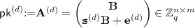
Next, encrypt bit-by-bit each secret key \( \mathsf {sk}^{(d)}\) using the sequentially following public key \( \mathsf {pk}^{(d+1)}\). Let \(\mathsf {Bit}_j( \mathsf {sk}^{(d)})\) denote the jth bit of \( \mathsf {sk}^{(d)}\). For every for every \(d\in [D]\) and \(j \in [n \cdot {\ell _q}]\) compute:
$$\overrightarrow{\mathcal {S}}^{(d)}[j] \leftarrow \mathsf {SHMK.Enc}( \mathsf {pk}^{(d+1)},\mathsf {Bit}_j( \mathsf {sk}^{(d)}))$$Finally, let the secret key be the last secret key of the sequence:
$$ \mathsf {sk}:= \mathsf {sk}^{(D+1)}$$And let the public key be the first public key of the sequence, along with the encryptions:
$$ \mathsf {pk}:= \left( \mathsf {pk}^{(1)},\overrightarrow{\mathcal {S}}^{(1)},\ldots ,\overrightarrow{\mathcal {S}}^{(D)}\right) $$ -
\(\mathsf {LMK.Enc}( \mathsf {pk},\mu )\): Sample uniformly at random \(\mathbf {r} \mathop {\leftarrow }\limits ^{\$} \{0,1\}^m\). Set and output the encryption:
$$\mathbf {c} := \mathbf {Ar} + \mu 2^{\ell -1}\mathbf {u}_n \in \mathbb {Z}_q^{n}$$ -
\(\mathsf {LMK.Dec}(( \mathsf {sk}_1,\ldots , \mathsf {sk}_N),c)\): Assume w.l.o.g that c is the product of evaluating a depth \(D\) circuit on newly encrypted ciphertexts (otherwise apply additional “dummy” homomorphic operations). Parse each secret key as \(\mathbf {{t}}_i = \mathbf {{t}}^{(D+1)}_i := \mathsf {sk}_i\) for every \(i \in [N]\). Concatenate the secret keys and set \(\widehat{\mathbf {{t}}} := (\mathbf {{t}}_1,\ldots ,\mathbf {{t}}_N) \in \mathbb {Z}_q^{nN}\). Compute and output
$$\mu ^\prime := \mathsf {Threshold}(\widehat{\mathbf {{t}}},\mathbf {{c}})$$

Evaluation is done similar to as described in Sect. 4.1. Consider evaluating a depth \(D\) circuit, and assume that the circuit is leveled, i.e. the gates of the circuit can be divided into \(D\) sets (levels) such that the first set is only fed by input gates, and set \(d+1\) is only fed by the outputs of gates in level \(d\). Clearly every circuit can be made leveled by adding dummy gates. Homomorphic evaluation maintains the invariant that an encryption w.r.t some set of users T at the input of level \(d\) is encrypted under their set of \( \mathsf {sk}^{(d)}\) keys. The computation of the gate is therefore performed w.r.t the set of \( \mathsf {sk}^{(d)}_i\) keys. Then for bootstrapping, we use the \(\mathbf {\mathcal {S}}^{(d)}_i\) key switching parameters, which allow us to produce an encryption of the bits of the \( \mathsf {sk}^{(d)}\) keys under the \( \mathsf {sk}^{(d+1)}\) keys, so the invariant is preserved. The noise growth is the same as analyzed in Lemma 7.
Security follows from LWE by a standard hybrid argument.
Lemma 9
The scheme described above is secure under the \(\mathrm {DLWE}_{n-1,q,\chi }\) assumption.
Following Corollary 3, we can assume \(\mathrm {DLWE}_{n-1,q,\chi }\) by assuming the quantum hardness of either \(\mathsf {GapSVP}_\gamma \) or \(\mathsf {SIVP}_\gamma \) for \(\gamma = \tilde{O}(nq/B_\chi )\). For bootstrapping to go through, we require that \(q/B_\chi = 2^{\omega (\log n)}\) (in fact, it is sufficient to have \(q/B_\chi = \mathrm{poly}(n,N)\), but we do not want to assume an upper bound on N, except that it’s some polynomial). As usual, we can scale \(q, B_\chi \) so long as their ratio remains large enough. This allows us to achieve better efficiency by scaling \(B_\chi ,q\) to be smallest possible, or achieving classical security by scaling q to be exponential in n, and \(B_\chi \) appropriately.
Rights and permissions
Copyright information
© 2016 International Association for Cryptologic Research
About this paper
Cite this paper
Brakerski, Z., Perlman, R. (2016). Lattice-Based Fully Dynamic Multi-key FHE with Short Ciphertexts. In: Robshaw, M., Katz, J. (eds) Advances in Cryptology – CRYPTO 2016. CRYPTO 2016. Lecture Notes in Computer Science(), vol 9814. Springer, Berlin, Heidelberg. https://doi.org/10.1007/978-3-662-53018-4_8
Download citation
DOI: https://doi.org/10.1007/978-3-662-53018-4_8
Published:
Publisher Name: Springer, Berlin, Heidelberg
Print ISBN: 978-3-662-53017-7
Online ISBN: 978-3-662-53018-4
eBook Packages: Computer ScienceComputer Science (R0)