Verifying a Verifier: On the Formal Correctness of an LTS Transformation Verification Technique

Abstract

Over the years, various formal methods have been proposed and further developed to determine the functional correctness of models of concurrent systems. Some of these have been designed for application in a model-driven development workflow, in which model transformations are used to incrementally transform initial abstract models into concrete models containing all relevant details. In this paper, we consider an existing formal verification technique to determine that formalisations of such transformations are guaranteed to preserve functional properties, regardless of the models they are applied on. We present our findings after having formally verified this technique using the Coq theorem prover. It turns out that in some cases the technique is not correct. We explain why, and propose an updated technique in which these issues have been fixed.

S. de Putter—This work is supported by ARTEMIS Joint Undertaking project EMC2 (grant nr. 621429).

1 Introduction

It is a well-known fact that concurrent systems are very hard to develop correctly. In order to support the development process, over the years, a whole range of formal methods techniques have been constructed to determine the functional correctness of system models [3]. Over time, these techniques have greatly improved, but the analysis of complex models is still time-consuming, and often beyond what is currently possible.

To get a stronger grip on the development process, model-driven development has been proposed [6]. In this approach, models are constructed iteratively, by defining model transformations that can be viewed as functions applicable on models: they are applied on models, producing new models. Using such transformations, an abstract initial model can be gradually transformed into a very detailed model describing all aspects of the system. If one can determine that the transformations are correct, then it is guaranteed that a correct initial model will be transformed into a correct final model.

Many model transformation verification techniques are focussed on determining that a given transformation applied on a given model produces a correct new model, but in order to show that a transformation is correct in general, one would have to determine this for all possible input models. There are some techniques that can do this [1, 11], but it is often far from trivial to show that these are correct.

In this work, we formally prove the correctness of such a formal transformation verification technique proposed in [17, 19] and implemented in the tool Refiner [20]. It is applicable on models with a semantics that can be captured by Labelled Transition Systems (LTSs). Transformations are formally defined as LTS transformation rules. Correctness of transformations is interpreted as the preservation of properties. Given a property $\varphi$ written in a fragment of the $\mu$-calculus [9], and a system of transformation rules $\varSigma$, Refiner checks whether $\varSigma$ preserves $\varphi$ for all possible input. This is done by first hiding all behaviour irrelevant for $\varphi$ [9] and then checking whether the rules replace parts of the input LTSs by new parts that are branching bisimilar to the old ones. Branching bisimilarity preserves safety properties and a subset of liveness properties involving inevitable reachability [5]. When no property is considered, the technique checks for full semantics preservation, useful, for instance, when refactoring models.

The technique has been successfully applied to reason very efficiently about model transformations; speedups of five orders of magnitude have been measured w.r.t. traditional model checking of the models the transformations are applied on [17]. However, the correctness of the transformation verification technique, i.e. whether it returns true iff a given transformation is property preserving for all possible input models, has been an open question until now. With this paper we address that issue.

Contributions. We address the formal correctness of the transformation verification technique from [19]. We have fully verified the correctness of this technique using the Coq proof assistant¹, and therefore present proofs in this paper that have been rigorously checked. The full proof is available at [10]. We have identified situations in which the technique is in fact not correct for certain cases. We propose two alterations to repair the identified issues: one involves a more rigorous comparison of combinations of glue-states (the states in the LTS patterns that need to be matched, but will not be transformed), and one means determining whether a rule system has a particular property which we call cascading.

Structure of the Paper. Related work is discussed in Sect. 2. Section 3 presents the notions for and analysis of the application of a single transformation rule. Next, in Sect. 4, the discussion is continued by considering networks of concurrent process LTSs, and systems of transformation rules. Two issues with the correctness of the technique in this setting are presented and solutions are proposed. Furthermore, we present a proof sketch along the lines of the Coq proof for the repaired technique. Finally, Sect. 5 contains our conclusions and pointers to future work.

2 Related Work

Papers on incremental model checking (IMC) propose how to reuse model checking results of safety properties for a given input model after it has been altered [14, 16]. We also consider verifying models that are subject to changes. However, we focus on analysing transformation specifications, i.e. the changes, themselves, allowing us to determine whether a change always preserves correctness, independent of the input model. Furthermore, our technique can also check the preservation of liveness properties.

In [12], an incremental algorithm is presented for updating bisimulation relations based on changes applied on a graph. Their goal is to efficiently maintain a bisimulation, whereas our goal is to assess whether bisimulations are guaranteed to remain after a transformation has been applied without considering the whole relation. As is the case for the IMC techniques, this algorithm works only for a given input graph, while we aim to prove correctness of the transformation specification itself regardless of the input.

In some works, e.g. [4, 15], theorem proving is used to verify the preservation of behavioural semantics. The use of theorem provers requires expert knowledge and high effort [15]. In contrast, our equivalence checking approach is more lightweight, automated, and allows the construction of counter-examples which help developers identify issues with the transformations.

In [2], transformation rules for Open Nets are verified on the preservation of dynamic semantics. Open Nets are a reactive extension of Petri Nets. The technique is comparable to the technique that we verify with two main exceptions. First, they consider weak bisimilarity for the comparison of rule patterns, which preserves a strictly smaller fragment of the $\mu$-calculus than branching bisimilarity [9]. Second, their technique does not allow transforming the communication interfaces between components. Our approach allows this, and checks whether the components remain ‘compatible’.

Finally, in [13], transformations expressed in the DSLTrans language are checked for correspondence between source and target models. DSLTrans uses a symbolic model checker to verify properties that can be derived from the meta-models. The state space captures the evolution of the input model. In contrast, our approach considers the state spaces of combinations of transformation rules, which represent the potential behaviour described by those rules. An interesting pointer for future work is whether those two approaches can be combined.

3 Verifying Single LTS Transformations

This section introduces the main concepts related to the transformation of LTSs, and explains how a single transformation rule can be analysed to guarantee that it preserves the branching structure of all LTSs it can be applied on.

3.1 LTS Transformation and LTS Equivalence

We use LTSs as in Definition 1 to reason about the potential behaviour of processes.

Definition 1

(Labelled Transition System). An LTS $\mathcal {G}$ is a tuple $( \mathcal {S}_{\mathcal {G}}, \mathcal {A}_{\mathcal {G}},$ $\mathcal {T}_{\mathcal {G}}, \mathcal {I}_{\mathcal {G}} )$, with

• $\mathcal {S}_{\mathcal {G}}$ a finite set of states;

• $\mathcal {A}_{\mathcal {G}}$ a set of action labels;

• $\mathcal {T}_{\mathcal {G}} \subseteq \mathcal {S}_{\mathcal {G}} \times \mathcal {A}_{\mathcal {G}} \times \mathcal {S}_{\mathcal {G}}$ a transition relation;

• $\mathcal {I}_{\mathcal {G}} \subseteq \mathcal {S}_{\mathcal {G}}$ a (non-empty) set of initial states.

Action labels in $\mathcal {A}_{\mathcal {G}}$ are denoted by a, b, c, etc. In addition, there is the special action label $\tau$ to represent internal, or hidden, system steps. A transition $( s, a, s' ) \in \mathcal {T}_{\mathcal {G}}$, or $s \xrightarrow {a}_\mathcal {G}s'$ for short, denotes that LTS $\mathcal {G}$ can move from state s to state $s'$ by performing the a-action. For the transitive reflexive closure of $\xrightarrow {a}_\mathcal {G}$, we use $\xrightarrow {a}\!\!^*_\mathcal {G}$. Note that transitions are uniquely identifiable by the combination of their source state, action label, and target state. This property is sometimes called the extensionality of LTSs [21].

We allow LTSs to be transformed by means of formally defined transformation rules. Transformation rules are defined as shown in Definition 2.

Definition 2

(Transformation Rule). A transformation rule $r = \langle \mathcal {L}, \mathcal {R}\rangle$ consists of a left pattern LTS $\mathcal {L}= \langle \mathcal {S}_{\mathcal {L}}, \mathcal {A}_{\mathcal {L}}, \mathcal {T}_{\mathcal {L}}, \mathcal {I}_{\mathcal {L}} \rangle$ and a right pattern LTS $\mathcal {R}= \langle \mathcal {S}_{\mathcal {R}}, \mathcal {A}_{\mathcal {R}}, \mathcal {T}_{\mathcal {R}}, \mathcal {I}_{\mathcal {R}} \rangle$, with $\mathcal {I}_{\mathcal {L}} = \mathcal {I}_{\mathcal {R}} = \mathcal {S}_{\mathcal {L}} \cap \mathcal {S}_{\mathcal {R}}$.

The states in $\mathcal {S}_{\mathcal {L}}\cap \mathcal {S}_{\mathcal {R}}$ are called the glue-states. When applying a transformation rule to an LTS, the changes are applied relative to these glue-states. For the verification we consider glue-states as initial states, i.e. $\mathcal {I}_{\mathcal {L}} = \mathcal {I}_{\mathcal {R}} = \mathcal {S}_{\mathcal {L}} \cap \mathcal {S}_{\mathcal {R}}$. A transformation rule $r = ( \mathcal {L}, \mathcal {R} )$ is applicable on an LTS $\mathcal {G}$ iff a match $m: \mathcal {L}\rightarrow \mathcal {G}$ exists according to Definition 3.

Definition 3

(Match). A pattern LTS $\mathcal {P}= ( \mathcal {S}_{\mathcal {P}}, \mathcal {A}_{\mathcal {P}}, \mathcal {T}_{\mathcal {P}}, \mathcal {I}_{\mathcal {P}} )$ has a match $m : \mathcal {P}\rightarrow \mathcal {G}$ on an LTS $\mathcal {G}= ( \mathcal {S}_{\mathcal {G}}, \mathcal {A}_{\mathcal {G}}, \mathcal {T}_{\mathcal {G}}, \mathcal {I}_{\mathcal {G}} )$ iff m is injective and $\forall s \in \mathcal {S}_{\mathcal {P}}\setminus \mathcal {I}_{\mathcal {P}}, p \in \mathcal {S}_{\mathcal {G}}$:

• $m(s) \xrightarrow {a}_{\mathcal {G}} p \implies (\exists s' \in \mathcal {S}_{\mathcal {P}}.\;s \xrightarrow {a}_{\mathcal {P}} s' \wedge m(s') = p);$

• $p \xrightarrow {a}_{\mathcal {G}}m(s) \implies (\exists s' \in \mathcal {S}_{\mathcal {P}}.\;s' \xrightarrow {a}_{\mathcal {P}} s \wedge m(s') = p)$.

A match is a behaviour preserving embedding of a pattern LTS $\mathcal {P}$ in an LTS $\mathcal {G}$ defined via a category of LTSs [21]. Moreover, a match may not cause removal of transitions that are not explicitly present in $\mathcal {P}$. The set $m(S)=\{m(s) \in \mathcal {S}_{\mathcal {G}} \mid s \in S \}$ is the image of a set of states S through match m on an LTS $\mathcal {G}$.

An LTS $\mathcal {G}$ is transformed to an LTS $T(\mathcal {G})$ according to Definition 4.

Definition 4

(LTS Transformation). Let $\mathcal {G}= \langle \mathcal {S}_{\mathcal {G}}, \mathcal {A}_{\mathcal {G}}, \mathcal {T}_{\mathcal {G}}, \mathcal {I}_{\mathcal {G}}\rangle$ be an LTS and let $r=\langle \mathcal {L}, \mathcal {R}\rangle$ be a transformation rule with match $m: \mathcal {L}\rightarrow \mathcal {G}$. Moreover, consider match $\hat{m}: \mathcal {R}\rightarrow T(\mathcal {G})$, with $\forall q \in \mathcal {S}_{\mathcal {L}}\cap \mathcal {S}_{\mathcal {R}}.\;\hat{m}(q) = m(q)$ and $\forall q \in \mathcal {S}_{\mathcal {R}}\setminus \mathcal {S}_{\mathcal {L}}.\;\hat{m}(q) \notin \mathcal {S}_{\mathcal {G}}$, defining the new states being introduced by the transformation. The transformation of LTS $\mathcal {G}$, via rule r with match $m$, is defined as $T(\mathcal {G}) = \langle \mathcal {S}_{T(\mathcal {G})}, \mathcal {A}_{T(\mathcal {G})}, \mathcal {T}_{T(\mathcal {G})}, \mathcal {I}_{\mathcal {G}}\rangle$ where

• $\mathcal {S}_{T(\mathcal {G})}= \mathcal {S}_{\mathcal {G}}\setminus m_\mathcal {L}(\mathcal {S}_{\mathcal {L}}) \cup m_\mathcal {R}(\mathcal {S}_{\mathcal {R}})$;

• $\mathcal {T}_{T(\mathcal {G})}= (\mathcal {T}_{\mathcal {G}}\setminus \{m_\mathcal {L}(s) \xrightarrow {a} m_\mathcal {L}(s') \mid s \xrightarrow {a}_\mathcal {L}s' \}) \cup \; \{m_\mathcal {R}(s) \xrightarrow {a} m_\mathcal {R}(s') \mid s \xrightarrow {a}_\mathcal {R}s' \}$

• $\mathcal {A}_{T(\mathcal {G})}= \{ a \mid \exists s \xrightarrow {a} s' \in \mathcal {T}_{T(\mathcal {G})}\}$

Fig. 1.

Application of a transformation rule

Given a match, an LTS transformation replaces states and transitions matched by $\mathcal {L}$ by a copy of $\mathcal {R}$ yielding LTS $T(\mathcal {G})$. Since in general, $\mathcal {L}$ may have several matches on $\mathcal {G}$, we assume that transformations are confluent, i.e. they are guaranteed to terminate and lead to a unique $T(\mathcal {G})$. Confluence of LTS transformations can be checked efficiently [18]. Assuming confluence means that when verifying transformation rules, we can focus on having a single match, since the transformations of individual matches do not influence each other. An application of a transformation rule is shown in Fig. 1. The initial and glue-states are coloured black. In the middle of Fig. 1, a transformation rule $r = ( \mathcal {L}, \mathcal {R} )$ is shown, which is applied on LTS $\mathcal {G}$ resulting in LTS $T(\mathcal {G})$. The states are numbered such that matches can be identified by the state label, i.e. a state $\tilde{i}$ is matched onto state i. The left-pattern of r does not match on states $\langle 1 \rangle$, $\langle 2 \rangle$, and $\langle 3 \rangle$ as this would remove the b-transition.

To compare LTSs, we use the branching bisimulation equivalence relation [5] as presented in Definition 5. Branching bisimulation supports abstraction from actions and is sensitive to internal actions and the branching structure of an LTS. Abstraction from actions is required for verification of abstraction and refinement transformations such that input and output models can be compared on the same abstraction level.

Definition 5

(Branching bisimulation). A binary relation B between two LTSs $\mathcal {G}_1$ and $\mathcal {G}_2$ is a branching bisimulation iff $s \;B\;t$ implies

Two states $s, t \in S$ are branching bisimilar, denoted $s \;\underline{\leftrightarrow }_b\;t$, iff there is a branching bisimulation B such that $s \;B\;t$. Two sets of states $S_1$ and $S_2$ are called branching bisimilar, denoted $S_1 \;\underline{\leftrightarrow }_b\;S_2$, iff $\forall s_1 \in S_1 . \exists s_2 \in S_2 . s_1 \;\underline{\leftrightarrow }_b\;s_2$ and vice versa. We say that two LTSs $\mathcal {G}_1$ and $\mathcal {G}_2$ are branching bisimilar, denoted $\mathcal {G}_1 \;\underline{\leftrightarrow }_b\;\mathcal {G}_2$, iff $\mathcal {I}_{\mathcal {G}_1} \;\underline{\leftrightarrow }_b\;\mathcal {I}_{\mathcal {G}_2}$.

3.2 Analysing a Transformation Rule

The basis of the transformation verification procedure is to check whether the two patterns making up a rule are equivalent, while respecting that the patterns share initial states. That is, given a rule $r = \langle \mathcal {L}, \mathcal {R}\rangle$, we are looking for a branching bisimulation relation R such that for all $s \in \mathcal {S}_{\mathcal {L}} \cap \mathcal {S}_{\mathcal {R}}$, we have $s\ R\ s$.

Fig. 2.

$\kappa$-loops ensure

Directly applying bisimilarity checking on a pair of LTSs, however, will not necessarily produce a suitable bisimulation relation. For instance, consider the rule in Fig. 2 which swaps a and b transitions. Without the $\kappa$-loops, explained in the next paragraph, the LTS patterns are branching bisimilar. However, the patterns should be interpreted as possible embeddings in larger LTSs. These larger LTSs may not be branching bisimilar, because glue-states $\langle \tilde{1} \rangle$ and $\langle \tilde{2} \rangle$ could be mapped to states with different in- and outgoing transitions, apart from the behaviour described in the LTS patterns.

To restrict bisimilarity checking to exactly those bisimulations that adhere to relating glue-states to themselves, we introduce a so-called $\kappa$-transition-loop for each glue-state, as defined in Definition 6. The resulting $\kappa$-extended transformation rule can now be defined as $r^\kappa = ( \mathcal {L}^\kappa , \mathcal {R}^\kappa )$, and is specifically used for the purpose of analysing r, it does not replace r. The $\kappa$-loop of a glue-state s is labelled with a unique label $\kappa _s \notin \mathcal {A}_{\mathcal {L}}\cup \mathcal {A}_{\mathcal {R}}$. If we add $\kappa$-loops to the rule in Fig. 2, the analysis is able to determine that the rule does not guarantee bisimilarity between input and output LTSs.

Definition 6

( $\kappa$ -extension of an LTS). The LTS $\mathcal {P}$ extended with $\kappa$-loops is defined as: $\mathcal {P}^{\kappa } = ( \mathcal {S}_{\mathcal {P}}, \mathcal {A}_{\mathcal {P}} \cup \{\kappa _s \mid s \in \mathcal {I}_{\mathcal {P}} \}, \mathcal {T}_{\mathcal {P}} \cup \{ ( s, \kappa _s, s ) \mid s \in \mathcal {I}_{\mathcal {P}}\}, \mathcal {I}_{\mathcal {P}} ) .$

The Analysis. A transformation rule preserves the branching structure of all LTSs it is applicable on if the patterns of a transformation rule extended with $\kappa$-loops are branching bisimilar. This is expressed in Proposition 1.

Proposition 1

Let $\mathcal {G}$ be an LTS, let r be a transformation rule with matches $m: \mathcal {L}\rightarrow \mathcal {G}$ and $\hat{m}: \mathcal {R}\rightarrow T(\mathcal {G})$ with $m(s)=\hat{m}(s)$ for all $s \in \mathcal {S}_{\mathcal {L}}\cap \mathcal {S}_{\mathcal {R}}$. Then,

Intuition. A match of pattern $\mathcal {L}$ is replaced with an instance of pattern $\mathcal {R}$. If $\mathcal {L}^\kappa \;\underline{\leftrightarrow }_b\;\mathcal {R}^\kappa$, then these two patterns exhibit branching bisimilar behaviour. Therefore, the behaviour of the original and transformed systems ($\mathcal {G}$ and $\mathcal {T}_{\mathcal {G}}$ respectively) are branching bisimilar.

4 Verifying Sets of Dependent LTS Transformations

In this section, we extend the setting by considering sets of interacting process LTSs in so-called networks of LTSs [7] or LTS networks. Transformations can now affect multiple LTSs in an input network, and the analysis of transformations is more involved, since changes to process-local behaviour may affect system-global properties. We address two complications that arose while trying to prove the correctness of the technique using Coq and propose how to fix the technique to overcome these problems. Finally, we provide a proof-sketch of the correctness of the fixed technique based on the complete Coq proof.

4.1 LTS Networks and Their Transformation

An LTS network (Definition 7) describes a system consisting of a finite number of concurrent process LTSs and a set of synchronisation laws which define the possible interaction between the processes. The explicit behaviour of an LTS network is defined by its system LTS (Definition 8). We write $1..n$ for the set of integers ranging from 1 to n. A vector $\bar{v}$ of size n contains n elements indexed from 1 to n. For all $i \in 1..n$, $\bar{v}_i$ represents the $i^{th}$ element of vector $\bar{v}$.

Definition 7

(LTS network). An LTS network $\mathcal {M}$ of size n is a pair $( \varPi , \mathcal {V} )$, where

• $\varPi$ is a vector of n concurrent LTSs. For each $i \in 1..n$, we write $\varPi _i = ( \mathcal {S}_{i}, \mathcal {A}_{i}, \mathcal {T}_{i}, \mathcal {I}_{i} )$.

• $\mathcal {V}$ is a finite set of synchronisation laws. A synchronisation law is a tuple $( \bar{t}, a )$, where $\bar{t}$ is a vector of size n, called the synchronisation vector, describing synchronising action labels, and a is an action label representing the result of successful synchronisation. We have $\forall i \in 1..n .\;\bar{t}_i \in \mathcal {A}_{i}\cup \{ \bullet \}$, where $\bullet$ is a special symbol denoting that $\varPi _i$ performs no action.

Definition 8

(System LTS). Given an LTS network $\mathcal {M}= ( \varPi , \mathcal {V} )$, its system LTS is defined by $\mathcal {G}_\mathcal {M}= ( \mathcal {S}_{\mathcal {M}}, \mathcal {A}_{\mathcal {M}}, \mathcal {T}_{\mathcal {M}}, \mathcal {I}_{\mathcal {M}} )$, with

• $\mathcal {S}_{\mathcal {M}}= \mathcal {S}_{1} \times \dots \times \mathcal {S}_{n}$;

• $\mathcal {A}_{\mathcal {M}}= \{ a \mid ( \bar{t}, a ) \in \mathcal {V}\}$;

• $\mathcal {I}_{\mathcal {M}}= \{ \langle s_1, \dots , s_n \rangle \mid s_i \in \mathcal {I}_{i}\}$, and

• $\mathcal {T}_{\mathcal {M}}$ is the smallest relation satisfying:

  

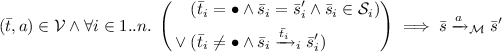
The system LTS is obtained by combining the processes in $\varPi$ according to the synchronisation laws in $\mathcal {V}$. The LTS network model subsumes most hiding, renaming, cutting, and parallel composition operators present in process algebras, but also more expressive operators such as m among n synchronisation [8]. For instance, hiding can be applied by replacing the a component in a law by $\tau$. A transition of a process LTS is cut if it is blocked with respect to the behaviour of the whole system (system LTS), i.e. there is no synchronization law involving the transition’s action label on the process LTS.

Figure 3 shows an LTS network $\mathcal {M}= ( \varPi , \mathcal {V} )$ with two processes and three synchronisation laws (left) and its system LTS (right). To construct the system LTS, first, the initial states of $\varPi _1$ and $\varPi _2$ are combined to form the initial state of $\mathcal {G}_\mathcal {M}$. Then, the outgoing transitions of the initial states of $\varPi _1$ and $\varPi _2$ are combined using the synchronisation laws, leading to new states in $\mathcal {G}_\mathcal {M}$, and so on. For simplicity, we do not show unreachable states.

Fig. 3.

An LTS network $\mathcal {M}= ( \varPi , \mathcal {V} )$ (left) and its system LTS $\mathcal {G}_\mathcal {M}$ (right)

Law $( \langle a, a \rangle , a )$ specifies that the process LTSs can synchronise on their a-transitions, resulting in a-transitions in the system LTS. The other laws specify that b- and d-transitions can synchronise, resulting in e-transitions, and that c-transitions can be fired independently. Note that in fact, b- and d-transitions in $\varPi _1$ and $\varPi _2$ are never able to synchronise.

The set of indices of processes participating in a synchronisation law $( \bar{t}, a )$ is formally defined as $Ac(\bar{t}) = \{ i \mid i \in 1..n \wedge \bar{t}_i \ne \bullet \}$; e.g. $Ac(\langle c, b, \bullet \rangle ) = \{1, 2\}$.

Branching bisimilarity is a congruence for construction of the system LTS of LTS networks if the synchronisation laws do not synchronise, rename, or cut $\tau$-transitions [7]. Given an LTS network $\mathcal {M}= ( \varPi , \mathcal {V} )$, these properties are formalised as follows:

• 1. $\forall ( \bar{t}, a ) \in \mathcal {V}, i \in 1..n .\;\bar{t}_i = \tau \implies Ac(\bar{t}) = \{i\}$ (no synchronisation of $\tau$’s);

• 2. $\forall ( \bar{t}, a ) \in \mathcal {V}, i \in 1..n .\;\bar{t}_i = \tau \implies a = \tau$ (no renaming of $\tau$’s);

• 3. $\forall i \in 1..n .\;\tau \in \mathcal {A}_{i} \implies \exists ( \bar{t}, a ) \in \mathcal {V}.\;\bar{t}_i = \tau$ (no cutting of $\tau$’s).

In this paper, we assume these properties hold.

Transformation of an LTS Network. A rule system is used to define transformations for LTS networks. A rule system $\varSigma$ is a tuple $( R, \mathcal {V}', \hat{\mathcal {V}} )$, where $R$ is a vector of transformation rules, $\mathcal {V}'$ is a set of synchronisation laws that must be present in networks that $\varSigma$ is applied on, and $\hat{\mathcal {V}}$ is a set of synchronisation laws introduced in the result of a transformation. A rule system $\varSigma = ( R, \mathcal {V}', \hat{\mathcal {V}} )$ is applicable on a given LTS network $\mathcal {M}= ( \varPi , \mathcal {V} )$ when for each synchronisation law in $\mathcal {V}'$ there is a synchronisation law in $\mathcal {V}$, and no other synchronisation laws in $\mathcal {V}$ involve behaviour described by the rules in $R$. As R is a vector, we identify transformation rules in R by an index. We write $\mathcal {L}_i$ and $\mathcal {R}_i$ for the left and right patterns, respectively, of rule $r_i$, where $i \in 1..|R|$.

Furthermore, the rule system must satisfy three analysis conditions related to transformation of synchronising behaviour in a network. The first condition concerns the applicability of a rule system on an LTS network. A rule transforming synchronising transitions must be applicable on all equivalent synchronising transitions:

Suppose $\varSigma$ is applied on a network $\mathcal {M}$ and $\varSigma$ contains a rule transforming synchronising a-transitions. If not all a-transitions are transformed it is unclear how this affects synchronisation between the processes, since the original and the transformed synchronising behaviour may coexist. The second and third conditions concern how a rule system is defined. The second condition requires that $\varSigma$ is complete w.r.t. synchronising behaviour.

For each action a synchronising with an action subjected to a rule there must be a rule also transforming a-transitions. This ensures that all the behaviour related to the synchronisation is captured in the rule system. Hence, the analysis considers a complete picture. For AC1 and AC2 the symmetric conditions involving the $\mathcal {R}$ and $\mathcal {V}'\cup \hat{\mathcal {V}}$ apply as well.

The third condition prevents that the new synchronisation laws in $\hat{\mathcal {V}}$ are defined over actions already present in the processes of an input network. Otherwise, a model could be altered without actually defining any transformation rules:

When transforming an LTS network $\mathcal {M}$ by means of a rule system $\varSigma$, first, we check whether $\varSigma$ is applicable on $\mathcal {M}$ and satisfies AC1. Then, for every $\varPi _i$ ($i \in 1..n$) and every $r \in R$, the largest set of matches is calculated. For each match, the corresponding transformation rule is applied. We call the resulting network $T_{\varSigma }(\mathcal {M})$. In contrast, when verifying a rule system, we first check that it is confluent and satisfies both AC2 and AC3. Checking confluence, AC1, AC2 and AC3 can be done efficiently [17–20].

4.2 Analysing Transformations of an LTS Network

In a rule system, transformation rules can be dependent on each other regarding the behaviour they affect. In particular, the rules may refer to actions that require synchronisation according to some law, either in the network being transformed, or the network resulting from the transformation. Since in general, it is not known a-priori whether or not those synchronisations can actually happen (see Fig. 3, the a-transitions versus the b- and d-transitions), full analysis of such rules must consider both successful and unsuccessful synchronisation.

To this end, dependent rules must be analysed in all possible combinations. Potential synchronisation between the behaviour in transformation rules is characterised by the direct dependency relation $D= \{(i, j) \mid \exists { ( \bar{t}, a ) \in \mathcal {V}'\cup \hat{\mathcal {V}}} .\;\{ i, j \}$ $\subseteq Ac(\bar{t}) \}$. Rule $r_i$ is related via $D$ to $r_j$ iff both rules participate in a synchronisation law. The relation considering directly and indirectly dependent rules, called the dependency relation, is defined by the transitive closure of $D$, i.e. $D^{+}$. The $D^{+}$ relation can be used to construct a partition $\mathbb {D}$ of the transformation rules into classes of dependent rules. Each class can be analysed independently. We call these classes dependency sets.

For the analysis of combinations of LTS patterns, we define in Definition 9 LTS networks $\bar{\mathcal {L}}^\kappa$ and $\bar{\mathcal {R}}^\kappa$ of $\kappa$-extended patterns, or pattern networks in short, consisting of a combination of the $\kappa$-extended left and right LTS patterns of a rule system $\varSigma$, respectively.

Definition 9

(( $\kappa$ -Extended) Pattern network). Given a rule system $\varSigma = ( R, \mathcal {V}', \hat{\mathcal {V}} )$, its left and right pattern networks are $\bar{\mathcal {L}}^\kappa$ and $\bar{\mathcal {R}}^\kappa$, respectively, where

In order to focus the analysis on combinations of dependent rules, we define how to filter an LTS network w.r.t. a given set I of indices. With the filtering operation, we can create filtered $\kappa$ -extended pattern networks $\mathcal {L}_I^{\kappa }$, $\mathcal {R}_I^{\kappa }$ for any set I of indices of dependent rules.

Definition 10

(Filtered LTS network). Given an LTS network $\mathcal {M}= ( \varPi , \mathcal {V} )$ of size n and a set of indices $I \subseteq 1..n$, the filtered LTS network is defined by $\mathcal {M}_I= (\varPhi , \mathcal {V}_\varPhi )$, with

where $*$ is a dummy state.

Next, we discuss the analysis of networks with focus on two areas in which the analysis technique as presented in [17, 19] was not correct. Firstly, the work did not consider the synchronisation of $\kappa$-transitions. Secondly, the consistency of synchronising behaviour across pattern networks was not considered.

Analysis of Pattern Networks and Synchronisation of $\kappa$ -Transitions. Figure 4a shows a rule system $\varSigma$, in which the two rules are dependent. The example demonstrates that the verification technique may produce incorrect results, since it does not consider synchronisations between $\kappa$-transitions. The corresponding pattern networks for $\varSigma$ are presented in Fig. 4b, if we ignore the last synchronisation law in $\mathcal {V}^\kappa$. The resulting bisimulation checks are given in Fig. 4c, if we ignore the $\kappa _{12}$-transitions. Unsuccessful synchronisation is considered in the checks between $\mathcal {L}^\kappa _{\{1\}}$ and $\mathcal {R}^\kappa _{\{1\}}$, and $\mathcal {L}^\kappa _{\{2\}}$ and $\mathcal {R}^\kappa _{\{2\}}$. In those, synchronisations are not possible (for instance between the z-transitions). The check between pattern networks $\mathcal {L}^\kappa _{\{1,2\}}$ and $\mathcal {R}^\kappa _{\{1,2\}}$ considers successful synchronisation. In the original verification technique [17, 19] the $\kappa _{12}$-loops in pattern networks $\mathcal {L}^\kappa _{\{1,2\}}$ and $\mathcal {R}^\kappa _{\{1,2\}}$ were not introduced. Without those loops, the pattern networks are branching bisimilar. However, as pattern networks may appear as an embedding in a larger network, all possible in- and outgoing transitions must be considered. Hence, synchronising transitions which enter and leave the pattern network must be considered as well. The $\kappa _{12}$-transitions in Fig. 4c are the result of synchronising $\kappa _1$ and $\kappa _2$-transitions, and therefore represent these synchronising transitions. Observe that in $\mathcal {R}^\kappa _{\{1,2\}}$ the possibility to perform $\kappa _{12}$-transitions is lost once the $\tau$-transition at state $\langle \tilde{1} , \tilde{2} \rangle$ has been taken, while in $\mathcal {L}^\kappa _{\{1,2\}}$ it is always possible to perform the $\kappa _{12}$-transition. Hence, the left and right networks are not branching bisimilar. These bisimulation checks show that $\varSigma$ does not guarantee preservation of the branching structure in all cases; e.g. take $( \varPi , \mathcal {V}' )$ as input network, with $\forall i \in 1..n .\;\varPi _i = \mathcal {L}_i$.

Fixing the Technique. To overcome the above mentioned shortcoming, we need to allow $\kappa$-transitions to synchronise. For this, additional $\kappa$-synchronisation laws must be introduced in the pattern networks by redefining $\mathcal {V}^\kappa$ in Definition 9 as follows:

For each vector glue-state $\bar{s}\in \mathcal {I}_{\mathcal {L}_I}$ ($I \subseteq 1..n$) there is now an enabled $\kappa$-synchronisation law. These $\kappa$-laws ensure that each vector of glue-states is at least related to itself.

Fig. 4.

A rule system and its pattern networks and bisimulation checks

Due to the $\kappa$-laws, groups of glue-states can be uniquely identified. This gives rise to Lemma 1 that states: if a state vector $\bar{s}\in \mathcal {S}_{\mathcal {L}_I}$, containing a group of glue-states, is related to a state vector $\bar{p}\in \mathcal {S}_{\mathcal {R}_I}$, then there must be a be a $\tau$-path from $\bar{p}$ to a state $\hat{\bar{p}} \in \mathcal {S}_{\mathcal {R}_I}$ such that $\hat{\bar{p}}$ and $\bar{s}$ are related, and $\hat{\bar{p}}$ contains the same group of glue-states as $\bar{s}$.

Lemma 1

Consider a rule system $\varSigma = ( R, \mathcal {V}', \hat{\mathcal {V}} )$ and sets of indices $I \subseteq 1..n$ and $J \subseteq I$. Let $\mathcal {L}_I$ and $\mathcal {R}_I$ be the corresponding pattern networks. Furthermore, let $B_{I}$ be a branching bisimulation relation such that $\mathcal {L}_I^{\kappa }\;\underline{\leftrightarrow }_b\;\mathcal {R}_I^{\kappa }$, then

Proof

Follows from the fact that $\bar{s}$ has a loop with a unique label, say $\kappa _{\bar{s}_J}$, identifying the group of glue-states. Hence, if $\bar{s}\;B_{I}\; \bar{p}$, then $\bar{p}$ must be able to perform a $\kappa _{\bar{s}_J}$-transition directly (i.e. $\forall i \in J .\;\bar{s}_i = \bar{p}_i$) or be able to reach such a transition via a $\tau$-path.    $\square$

Consistency of Synchronising Behaviour. Formal verification of the analysis technique in Coq furthermore showed that in one other case, the technique also incorrectly concludes that a rule system is correct for all possible input. This happens when a rule system is not behaviourally consistent across pattern networks. Consider a rule system $\varSigma$ with two transformation rules such that $\mathcal {L}^\kappa _{\{1,2\}} \;\underline{\leftrightarrow }_b\;\mathcal {R}^\kappa _{\{1,2\}}$, $\mathcal {L}^\kappa _{\{1\}} \;\underline{\leftrightarrow }_b\;\mathcal {R}^\kappa _{\{1\}}$, and $\mathcal {L}^\kappa _{\{2\}} \;\underline{\leftrightarrow }_b\;\mathcal {L}^\kappa _{\{2\}}$. Furthermore, consider vector states $\langle t_\mathcal {L} , g \rangle \in \mathcal {S}_{\mathcal {L}^\kappa _{\{1,2\}}}$ and $\langle t_\mathcal {R} , g \rangle \in \mathcal {S}_{\mathcal {R}^\kappa _{\{1,2\}}}$ such that $\langle t_\mathcal {L} , g \rangle \;\underline{\leftrightarrow }_b\; \langle t_\mathcal {R} , g \rangle$, where g is a glue-state. When we also have $t_\mathcal {L}\;\underline{\leftrightarrow }_b\;t_\mathcal {R}$ we say that this relation cascades from the relation between $\langle t_{\mathcal {L}} , g \rangle$ and $\langle t_\mathcal {R} , g \rangle$. If such a cascading effect holds for all states across different combinations of pattern networks, then the rule system is said to be cascading, i.e. it is behaviourally consistent across the pattern networks. A formal definition is given in Definition 11.

Definition 11

(Cascading rule system). A rule system $\varSigma = ( R, \hat{\mathcal {V}} )$ with synchronisation vectors of size n is called cascading, iff for all sets of indices $I, J \subseteq 1..n$ with $I \cap J = \emptyset$:

where $\bar{x} \parallel \bar{y}$ is the merging of states $\bar{x}$ and $\bar{y}$ via vector addition with dummy state ${*}$ as the zero element. Intuitively, this operation constructs a state for the system LTS considering LTS patterns indexed by $I \cup J$, i.e. the parallel composition of $\bar{x}$ and $\bar{y}$.

It may be the case that $\varSigma$ is not cascading, i.e. we have $\langle t_\mathcal {L} , g \rangle \;\underline{\leftrightarrow }_b\; \langle t_\mathcal {R} , g \rangle$, but not . In such a case it is always possible to construct an input LTS network $\mathcal {M}$ such that . To construct $\mathcal {M}$ take a copy of $\mathcal {L}_{\{1,2\}}$ and add a transition $g \xrightarrow {d}_2 s$, where s is a state that is not matched by $\mathcal {L}_1$ and the d-transition signifies departure from the pattern network. We have $\langle t_\mathcal {L} , g \rangle \xrightarrow {d}_\mathcal {M} \langle t_\mathcal {L} , s \rangle$ and $\langle t_\mathcal {R} , g \rangle \xrightarrow {d}_{T_{\varSigma }(\mathcal {M})} \langle t_\mathcal {R} , s \rangle$. To represent continuing behaviour in $\varPi _1$ (copy of ) we add a selfloop $t_\mathcal {L}\xrightarrow {a}_1 t_\mathcal {L}$ where a is a unique action. Since state s is not matched and , it follows that $\langle t_\mathcal {L} , s \rangle$ can perform the a-loop while $\langle t_\mathcal {R} , s \rangle$ cannot. Hence, we have .

Figure 5a presents a transformation of an LTS network $\mathcal {M}$ using a non-cascading rule system $\varSigma$. The corresponding bisimulation checks are shown in Fig. 5b. The rule system is not cascading since state $\langle \tilde{1} \rangle$ is not related to state $\langle \tilde{4} \rangle$, while $\langle \tilde{1} , \tilde{2} \rangle \;\underline{\leftrightarrow }_b\; \langle \tilde{4} , \tilde{2} \rangle$. The matches of the latter states (i.e. $\langle 1 , 2 \rangle$ and $\langle 4 , 2 \rangle$) can perform a d-transition to states $\langle 1 , 3 \rangle$ and $\langle 4 , 3 \rangle$, respectively. However, state $\langle 1 , 3 \rangle$ can perform an a-loop while state $\langle 4 , 3 \rangle$ cannot. In other words, states $\langle \tilde{1} , \tilde{2} \rangle$ and $\langle \tilde{4} , \tilde{2} \rangle$ are branching bisimilar, but their matched states $\langle 1 , 2 \rangle$ and $\langle 4 , 2 \rangle$ are clearly not. Hence, the bisimulation checks fail to establish that $\varSigma$ does not guarantee $\mathcal {M}\;\underline{\leftrightarrow }_b\;T_{\varSigma }(\mathcal {M})$ for arbitrary $\mathcal {M}$.

Fig. 5.

A transformation using a non-cascading rule system does not preserve the branching structure of LTS network $\mathcal {M}$

Fig. 6.

The revised check recognises that the non-cascading rule system does not preserve the branching structure of input networks:

Fixing the Technique. To overcome this shortcoming, we propose, instead of $\kappa$-loops, to introduce a $\kappa$ -state in the $\kappa$-extension of an LTS pattern with $\kappa$-transitions from and to all glue-states. The $\kappa$-state represents all states that have transitions to and from (but are themselves not present in) matches of LTS patterns. This captures the possibility of leaving a match of a pattern network and ending up in a sub-state which is not related through the cascading effect. The $\kappa$-state extended version of Fig. 5b is presented in Fig. 6. The (vector) states containing $\kappa$-states are coloured grey. In the new situation, the lack of the cascading effect in $\varSigma$ becomes visible through checking branching bisimilarity. We implemented this approach in Refiner, and observed no extra runtime overhead.

The Analysis. Checking a rule system $\varSigma = ( R, \mathcal {V}', \hat{\mathcal {V}} )$ now proceeds as follows:

• 1. Check whether in $\varSigma$, no $\tau$-transitions can be synchronised, renamed, or cut, and whether $\varSigma$ satisfies AC2 and AC3. If not, report this and stop.

• 2. Extend the patterns of each rule in R with a $\kappa$-state and $\kappa$-transitions between the $\kappa$-state and the glue-states.

• 3. Construct the set of dependency sets $\mathbb {D}$.

• 4. For each class (dependency set) $P \in \mathbb {D}$, and each non-empty subset $P' \subseteq P$:

  • (a) Combine the patterns of rules in $P'$ into networks $\mathcal {L}_{P'}^\kappa$, $\mathcal {R}_{P'}^\kappa$, respectively.

  • (b) Determine whether $\mathcal {L}_{P'}^\kappa \;\underline{\leftrightarrow }_b\;\mathcal {R}_{P'}^\kappa$ holds.

If 4b only gives positive results, then $\varSigma$ is branching-structure preserving for all inputs it is applicable on. At step 4, all non-empty subsets of dependency sets are considered. Proper subsets represent unsuccessful synchronisation situations. Proposition 2 formally describes the technique. The full proof in the form of Coq code can be found at [10]. Here we present a proof sketch.

To show the correctness of Proposition 2, we have to define a branching bisimulation relation relating the original and transformed LTS networks. To simplify the proof, we assume that $\varSigma$ has n rules, and that a rule r with index i, denoted as $r_i$, matches on $\varPi _i$ in the LTS network that $\varSigma$ is applied on. For confluent rule systems, the result can be lifted to the general case where rules can match arbitrary process LTSs. Moreover, we want to relate the matched elements of vector states via their corresponding pattern networks. For this we define a set of indices of elements in vector state $\bar{s}$ matched on by the corresponding transformation rule, i.e. $M(\bar{s})= \{ i \mid \bar{s}_i \in m_i(\mathcal {S}_{\mathcal {L}_i}) \cup \hat{m}_i(\mathcal {S}_{\mathcal {R}_i}) \}$. With this set the elements of a vector state with transformed behaviour can be selected.

Furthermore, we introduce a mapping of state vectors. Similar to matches for a single rule, the mapping of a state vector of a pattern network defines how it is mapped to a state vector of an LTS network. By referring to matches of the individual vector elements, a state vector is mapped on to another state vector. Consider an LTS network $\mathcal {M}= ( \varPi , \mathcal {V} )$ of size n and a pattern network $\mathcal {M}_I= ( \varPi _I, \mathcal {V}_I )$ with $I \subseteq 1..n$. We say a vector state $\bar{q}\in \mathcal {S}_{\mathcal {M}_I}$ is mapped to a state $\bar{s}\in \mathcal {S}_{\mathcal {M}}$, denoted by $\bar{q} \vdash _{I} \bar{s}$, iff $\forall i \in I .\;m(\bar{q}_i) = \bar{s}_i$. Mapping $\bar{q} \vdash _{I} \bar{s}$ amounts to a simulation relation between the state vectors: the group of states $\bar{s}_i$ indexed by $i \in I$ can simulate the behaviour of state vector $\bar{q}$.

Proposition 2

Let $\mathcal {M}= ( \varPi , \mathcal {V} )$ be an LTS network of size n and let $\varSigma = ( R, \mathcal {V}', \hat{\mathcal {V}} )$ be a cascading rule system satisfying AC2 and AC3. Let $\bar{r}$ be a vector of size n such that for all $i \in 1..n$, $\bar{r}_i \in R$ with corresponding matches $m_i: \mathcal {L}_i\rightarrow \varPi _i$ and $\hat{m}_i: \mathcal {R}_i\rightarrow T(\varPi _i)$. Then,

Proof Sketch. By definition, we have $\mathcal {M}\;\underline{\leftrightarrow }_b\;T_{\varSigma }(\mathcal {M})$ iff there exists a branching bisimulation relation C with $\mathcal {I}_{\mathcal {M}}\;\underline{\leftrightarrow }_b\;\mathcal {I}_{T_{\varSigma }(\mathcal {M})}$. Branching bisimilarity is a congruence for the construction of system LTSs from LTS networks, i.e. two pairs of pattern networks $\mathcal {L}_I$ and $\mathcal {R}_I$, $\mathcal {L}_J$ and $\mathcal {R}_J$, with $\mathcal {L}_I \;\underline{\leftrightarrow }_b\;\mathcal {R}_I$ and $\mathcal {L}_J \;\underline{\leftrightarrow }_b\;\mathcal {R}_J$, can be combined to form pattern networks $\mathcal {L}_{I\cup J}$ and $\mathcal {R}_{I \cup J}$ such that $\mathcal {L}_{I\cup J} \;\underline{\leftrightarrow }_b\;\mathcal {R}_{I \cup J}$. Therefore, we have $\forall I \subseteq 1..n .\;\mathcal {L}^\kappa _I \;\underline{\leftrightarrow }_b\;\mathcal {R}^\kappa _I$ and we can avoid reasoning about the dependency sets in $\mathbb {D}$. As a consequence, for any $I \subseteq 1..n$ there exists a branching bisimulation relation $B_{I}$ with $\mathcal {I}_{\mathcal {L}_I^{\kappa }} \;\underline{\leftrightarrow }_b\;\mathcal {I}_{\mathcal {R}_I^{\kappa }}$. We define $C$ as follows:

The first case in the relation, $i \notin M(\bar{s})\cup M(\bar{p})$, relates the sub-states of a state vector that are not matched by transformation rules. The second case, $i \in M(\bar{s})\cup M(\bar{p})$, relates the matched sub-states of a state vector. Because of the way that C is constructed we have that if $s \;C\;p$, then $M(\bar{s}) = M(\bar{p})$. For brevity, we will write $M(\bar{s})$ instead of $M(\bar{s}) \cup M(\bar{p})$.

To prove the proposition we have to show that $C$ is a bisimulation relation. This requires proving that $C$ relates the initial states of $\mathcal {M}$ and $T_{\varSigma }(\mathcal {M})$ and that $C$ satisfies Definition 5 as presented below.

$\bullet \;$ $C$ relates the initial states of $\mathcal {M}$ and $T_{\varSigma }(\mathcal {M})$, i.e. $\mathcal {I}_{\mathcal {M}} \;C\; \mathcal {I}_{T_{\varSigma }(\mathcal {M})}$. We have $\mathcal {I}_{\mathcal {M}}= \mathcal {I}_{T_{\varSigma }(\mathcal {M})}$. Initial states are not removed by the transformation. Furthermore, if states are matched on initial states, then the matching states are glue-states according to Definition 3. For $i \in M(\bar{s})$ glue-states are related to themselves. Furthermore, for $i \notin M(\bar{s})$ the sub-state is not touched by the transformation. Hence, $C$ relates the initial states.

$\bullet \;$ If $\bar{s}\;C\;\bar{p}$ and $\bar{s}\xrightarrow {a}_{\mathcal {M}} \bar{s}'$ then either $a = \tau \wedge \bar{s}'\;C\;\bar{p}$, or $\bar{p}\Rightarrow _{T_{\varSigma }(\mathcal {M})} \hat{\bar{p}} \xrightarrow {a}_{T_{\varSigma }(\mathcal {M})} \bar{p}'\wedge \bar{s}\;C\;\hat{\bar{p}} \wedge \bar{s}'\;C\;\bar{p}'$. Consider synchronisation law $( \bar{t}, a ) \in \mathcal {V}$ enabling the transition $\bar{s}\xrightarrow {a}_{\mathcal {M}} \bar{s}'$. We distinguish two cases:

• 1. There exists $i \in Ac(\bar{t})$ such that transition $\bar{s}\xrightarrow {\bar{t}_i}_{\varPi _i} \bar{s}'$ is matched. By analysis conditions (AC1) and (AC2), for all $i \in Ac(\bar{t})$ there must be a transition matching $\bar{s}\xrightarrow {\bar{t}_i}_{\varPi _i} \bar{s}'$. Hence, we have $Ac(\bar{t}) \subseteq M(\bar{s})$ and a transition matching $\bar{s}\xrightarrow {a}_{\mathcal {M}} \bar{s}'$. Since the transition is matched there exists $\bar{s}_m, \bar{s}'_m \in \mathcal {S}_{\mathcal {L}_M(\bar{s})}$ and $\bar{p}_m \in \mathcal {S}_{\mathcal {R}_M(\bar{s})}$ with $\bar{s}_m \vdash _{M(\bar{s})} \bar{s}$, $\bar{p}_m \vdash _{M(\bar{s})} \bar{p}$, $\bar{s}_m \;B_{M(\bar{s})}\; \bar{p}_m$ and $\bar{s}\xrightarrow {a}_{\mathcal {L}_{M(\bar{s})}} \bar{s}'$ (by Definition of $C$). Since $\bar{s}_m \;B_{M(\bar{s})}\; \bar{p}_m$, by Definition 5, we have:

  • $a = \tau$ with $\bar{s}'_m \;B_{M(\bar{s})}\; \bar{p}_m$. We have to show $\bar{s}'\;C\;\bar{p}$, which follows from def. of $C$ and Definition 8 (system LTS).

  • $\bar{p}_m \xrightarrow {\tau }\!\!^*_{\mathcal {R}_M(\bar{s})} \hat{\bar{p}}_m \xrightarrow {a}_{\mathcal {R}_M(\bar{s})} \bar{p}'$ with $\bar{s}_m \;B_{M(\bar{s})}\; \hat{\bar{p}}_m$ and $\bar{s}'_m \;B_{M(\bar{s})}\; \bar{p}'_m$. We construct states $\hat{\bar{p}}$ and $\bar{p}'$ such that $\bar{p}\xrightarrow {\tau }\!\!^*_{T_{\varSigma }(\mathcal {M})} \hat{\bar{p}} \xrightarrow {a}_{T_{\varSigma }(\mathcal {M})} \bar{p}'$ and $\bar{s}\;C\;\hat{\bar{p}}$. Finally, $\bar{s}'\;C\;\bar{p}'$ follows from def. of $C$ and Definition 8 (system LTS).

• 2. There is no transition matching $\bar{s}\xrightarrow {a}_{\mathcal {M}} \bar{s}'$. We distinguish two cases:

  • (a) One or more active sub-states of $\bar{s}$ are matched on, i.e. $Ac(\bar{t}) \cap M(\bar{s})\ne \emptyset$. Since the transition is not matched the active sub-states of $\bar{s}$ must be matches of glue-states. By Lemma 1, we have states $\hat{\bar{p}}$ and $\bar{p}'$ such that $\bar{p}\xrightarrow {\tau }\!\!^*_{T_{\varSigma }(\mathcal {M})} \hat{\bar{p}} \xrightarrow {a}_{T_{\varSigma }(\mathcal {M})} \bar{p}'$ and $\bar{s}\;C\;\hat{\bar{p}}$. Left to show is $\bar{s}'\;C\;\bar{p}'$. Let $i \in 1..n$:

    • $i\notin M(\bar{s})$. By construction of $\bar{p}'$ it follows that $\bar{s}'_i = \bar{p}'_i$.

    • $i\in M(\bar{s})$. Only sub-states index by $Ac(\bar{t})$ change. Sub-states index by $Ac(\bar{t})$ may have a transition from a matched sub-state to another matched sub-state, or such a matched sub-state may transition to a sub-state that is not matched (or vice versa). We construct states $\bar{s}'\in \mathcal {S}_{\mathcal {L}_{M(\bar{s}')}}$ and $\bar{p}'\in \mathcal {S}_{\mathcal {R}_{M(\bar{s}')}}$ by considering the two disjoint sets $M(\bar{s}')\setminus Ac(\bar{t})$ and $M(\bar{s}')\cap Ac(\bar{t})$. For the first set we can construct two states $\bar{s}_{mJ}$ and $\bar{p}_{mJ}$ that, because of Definition 11 (cascading rule system), are related by $B_{M(\bar{s}')\setminus Ac(\bar{t})}$. From sub-states of $\bar{s}_m$ indexed by the second set we can construct a state $\bar{q}\in \mathcal {I}_{\mathcal {L}_{M(\bar{s}')\cap Ac(\bar{t})}}$. Because glue-state are related to themselves we have $\bar{q}\;B_{M(\bar{s}')\cap Ac(\bar{t})}\; \bar{q}$. From $\bar{s}_{mJ}$, $\bar{p}_{mJ}$, and $\bar{q}$ we can construct states $\bar{s}'_m$ and $\bar{p}'_m$ such that $\bar{s}'_m \;B_{M(\bar{s}')}\; \bar{p}_m$ (by Definition 11).

  • (b) No active sub-states of $\bar{s}$ are matched on, i.e. $Ac(\bar{t}) \cap M(\bar{s})= \emptyset$. We construct a state $\bar{p}'\in \mathcal {S}_{T_{\varSigma }(\mathcal {M})}$ from $\bar{p}$ and the active sub-states of $\bar{s}'$ such that $\bar{p}\xrightarrow {a}_{T_{\varSigma }(\mathcal {M})} \bar{p}'$. Left to show $\bar{s}'\;C\;\bar{p}'$. Considering an $i \in 1..n$ we have to distinguish the following cases:

    • $i \notin M(\bar{s})$. We have to show that $\bar{s}'_i = \bar{p}'_i$, this can be derived from, $\bar{s}\;C\;\bar{p}$, Definition 8 (system LTS), and construction of $\bar{p}'$.

    • $i \in M(\bar{s})$. To relate $\bar{s}'$ and $\bar{p}'$ we need to find a relation $B_{M(\bar{s}')}$ relating two states that map on $\bar{s}'$ and $\bar{p}'$ respectively. If only active sub-states of $\bar{s}'$ are matched we can use the property that initial states are related to themselves in $B_{M(\bar{s}')}$. In the opposite case, there is a $j \in 1..n \setminus Ac(\bar{t})$ and we can use $\bar{s}\;C\;\bar{p}$ to construct the required relation.

$\bullet \;$ The symmetric case: if $\bar{s}\;C\;\bar{p}$ and $\bar{p}\xrightarrow {a}_{\mathcal {M}} \bar{p}'$ then either $a = \tau \wedge \bar{s}'\;C\;\bar{p}$, or $\bar{s}\Rightarrow _{\mathcal {M}} \hat{\bar{s}} \xrightarrow {a}_{\mathcal {M}} \bar{s}'\wedge \bar{s}\;C\;\hat{\bar{p}} \wedge \bar{s}'\;C\;\bar{p}'$.

This case is symmetric to the previous case with the exception that $\bar{p}\xrightarrow {a}_{T(\mathcal {M})} \bar{p}'$ is enabled by some $( \bar{t}, a ) \in \mathcal {V}\cup \hat{\mathcal {V}}$. Therefore, when transition $\bar{p}\xrightarrow {a}_{T(\mathcal {M})} \bar{p}'$ is not matched on, we have to show that $( \bar{t}, a ) \in \mathcal {V}$. Let $\bar{p}, \bar{p}'\in \mathcal {S}_{T_{\varSigma }(\mathcal {M})}$ such that $\bar{p}\xrightarrow {a}_{T(\mathcal {M})} \bar{p}'$ is enabled by some $( \bar{t}, a ) \in \mathcal {V}\cup \hat{\mathcal {V}}$. Furthermore, transition $\bar{p}\xrightarrow {a}_{T(\mathcal {M})} \bar{p}'$ is not matched on. Assume for a contradiction that $( \bar{t}, a ) \in \hat{\mathcal {V}}$. Since $( \bar{t}, a ) \in \hat{\mathcal {V}}$ is introduced by the transformation , by (AC3), there must be an i such that $\bar{t}_i \in \mathcal {A}_{\mathcal {R}_i} \setminus \mathcal {A}_{\mathcal {L}_i}$. It follows that there is a transition matching $\bar{p}\xrightarrow {a}_{T(\mathcal {M})} \bar{p}'$ contradicting our earlier assumption. Hence, we must have $( \bar{t}, a ) \in \mathcal {V}$.    $\square$

5 Conclusions

We discussed the correctness of an LTS transformation verification technique. The aim of the technique is to verify whether a given LTS transformation system $\varSigma$ preserves a property $\varphi$, written in a fragment of the $\mu$-calculus, for all possible input models formalised as LTS networks. It does this by determining whether $\varSigma$ is guaranteed to transform an input network into one that is branching bisimilar, ignoring the behaviour not relevant for $\varphi$.

It turned out that the technique was not correct for two reasons: (1) it ignored potentially synchronising behaviour connected to the glue-states of rules, but not part of the rule patterns, and (2) it did not check whether the rule system is cascading. We proposed how to repair the technique and presented a proof-sketch of its correctness. A complete proof has been carried out in Coq.

Future Work. Originally divergence-sensitive branching bisimulation was used [19], which preserves $\tau$-loops and therefore liveness properties. In future work, we would like to prove that for this flavour of bisimulation the technique is also correct. Moreover, we would like to investigate what the practical limitations of the pre-conditions of the technique are in industrial sized transformation systems.

Finally, in [17], the technique from [19] has been extended to explicitly consider the communication interfaces between components, thereby removing the completeness condition AC2 regarding synchronising behaviour being transformed (see Sect. 4.1). We wish to prove that also this extension is correct.

References

Amrani, M., Combemale, B., Lúcio, L., Selim, G.M.K., Dingel, J., Le Traon, Y., Vangheluwe, H., Cordy, J.R.: Formal verification techniques for model transformations: a tridimensional classification. JOT 14(3), 1–43 (2015)
Baldan, P., Corradini, A., Ehrig, H., Heckel, R., König, B.: Bisimilarity and behaviour-preserving reconfigurations of open petri nets. In: Mossakowski, T., Montanari, U., Haveraaen, M. (eds.) CALCO 2007. LNCS, vol. 4624, pp. 126–142. Springer, Heidelberg (2007)
Bowen, J., Hinchey, M.: Formal methods. In: Tucker, A.B. (ed.) Computer Science Handbook Chap. 106, pp. 106-1–106-25. ACM, New York (2004)
Giese, H., Glesner, S., Leitner, J., Schäfer, W., Wagner, R.: Towards verified model transformations. In: MoDeVVa 2006, pp. 78–93 (2006)
van Glabbeek, R.J., Weijland, W.P.: Branching time and abstraction in bisimulation semantics. J. ACM 43(3), 555–600 (1996)
Kleppe, A., Warmer, J., Bast, W.: MDA Explained: The Model Driven Architecture(TM): Practice and Promise. Addison-Wesley Professional, Boston (2005)
Lang, F.: Refined interfaces for compositional verification. In: Najm, E., Pradat-Peyre, J.-F., Donzeau-Gouge, V.V. (eds.) FORTE 2006. LNCS, vol. 4229, pp. 159–174. Springer, Heidelberg (2006)
Lang, F., Mateescu, R.: partial model checking using networks of labelled transition systems and boolean equation systems. Log. Methods Comput. Sci. 9(4), 1–32 (2013)
Mateescu, R., Wijs, A.: Property-dependent reductions adequate with divergence-sensitive branching bisimilarity. Sci. Comput. Prog. 96(3), 354–376 (2014)
de Putter, S.: Coq code proving the correctness of the LTS transformation verification technique (2015). http://www.mdsetechnology.org/attachments/article/2/FASE16_property_preservation.zip
Rahim, L.A., Whittle, J.: A survey of approaches for verifying model transformations. Softw. Syst. Model. 14, 1–26 (2013). http://dx.doi.org/10.1007/s10270-013-0358-0
Saha, D.: An incremental bisimulation algorithm. In: Arvind, V., Prasad, S. (eds.) FSTTCS 2007. LNCS, vol. 4855, pp. 204–215. Springer, Heidelberg (2007)
Selim, G.M.K., Lúcio, L., Cordy, J.R., Dingel, J., Oakes, B.J.: Specification and verification of graph-based model transformation properties. In: Giese, H., König, B. (eds.) ICGT 2014. LNCS, vol. 8571, pp. 113–129. Springer, Heidelberg (2014)
Sokolsky, O., Smolka, S.: Incremental model checking in the modal mu-calculus. In: Dill, D.L. (ed.) Computer Aided Verification. LNCS, vol. 818, pp. 351–363. Springer, Heidelberg (1994)
Stenzel, K., Moebius, N., Reif, W.: Formal verification of QVT transformations for code generation. In: Whittle, J., Clark, T., Kühne, T. (eds.) MODELS 2011. LNCS, vol. 6981, pp. 533–547. Springer, Heidelberg (2011)
Swamy, G.: Incremental methods for formal verification and logic synthesis. Ph.D. thesis, University of California (1996)
Wijs, A.: Define, verify, refine: correct composition and transformation of concurrent system semantics. In: Fiadeiro, J.L., Liu, Z., Xue, J. (eds.) FACS 2013. LNCS, vol. 8348, pp. 348–368. Springer, Heidelberg (2014)
Wijs, A.J.: Confluence detection for transformations of labelled transition systems. In: GaM 2015. EPTCS, vol. 181, pp. 1–15. Open Publishing Association (2015)
Wijs, A., Engelen, L.: Efficient property preservation checking of model refinements. In: Piterman, N., Smolka, S.A. (eds.) TACAS 2013 (ETAPS 2013). LNCS, vol. 7795, pp. 565–579. Springer, Heidelberg (2013)
Wijs, A., Engelen, L.: REFINER: towards formal verification of model transformations. In: Badger, J.M., Rozier, K.Y. (eds.) NFM 2014. LNCS, vol. 8430, pp. 258–263. Springer, Heidelberg (2014)
Winskel, G.: A Compositional proof system on a category of labelled transition systems. Inf. Comput. 87(1–2), 2–57 (1990)
Author information
Authors and Affiliations
Corresponding author
Editor information
Editors and Affiliations
Rights and permissions
Copyright information
© 2016 Springer-Verlag Berlin Heidelberg
About this paper
Cite this paper
de Putter, S., Wijs, A. (2016). Verifying a Verifier: On the Formal Correctness of an LTS Transformation Verification Technique. In: Stevens, P., Wąsowski, A. (eds) Fundamental Approaches to Software Engineering. FASE 2016. Lecture Notes in Computer Science(), vol 9633. Springer, Berlin, Heidelberg. https://doi.org/10.1007/978-3-662-49665-7_23
Download citation
DOI: https://doi.org/10.1007/978-3-662-49665-7_23
Publisher Name: Springer, Berlin, Heidelberg
Print ISBN: 978-3-662-49664-0
Online ISBN: 978-3-662-49665-7
eBook Packages: Computer ScienceComputer Science (R0)