Functional Encryption Without Obfuscation

Abstract

Previously known functional encryption (FE) schemes for general circuits relied on indistinguishability obfuscation, which in turn either relies on an exponential number of assumptions (basically, one per circuit), or a polynomial set of assumptions, but with an exponential loss in the security reduction. Additionally most of these schemes are proved in the weaker selective security model, where the adversary is forced to specify its target before seeing the public parameters. For these constructions, full security can be obtained but at the cost of an exponential loss in the security reduction.

In this work, we overcome the above limitations and realize an adaptively secure functional encryption scheme without using indistinguishability obfuscation. Specifically the security of our scheme relies only on the polynomial hardness of simple assumptions on composite order multilinear maps. Though we do not currently have secure instantiations for these assumptions, we expect that multilinear maps supporting these assumptions will discovered in the future. Alternatively, follow up results may yield constructions which can be securely instantiated.

As a separate technical contribution of independent interest, we show how to add to existing graded encoding schemes a new extension function, that can be thought of as dynamically introducing new encoding levels.

S. Garg—Work supported in part from a DARPA/ARL SAFEWARE award, AFOSR Award FA9550-15-1-0274, and NSF CRII Award 1464397. The views expressed are those of the authors and do not reflect the official policy or position of the Department of Defense, the National Science Foundation, or the U.S. Government.

M. Zhandry—Work done while the author was a graduate student at Stanford University. Supported by the DARPA PROCEED program.

1 Introduction

In traditional encryption schemes, decryption control is all or nothing: the sender encrypts its message under a particular key, and anyone with the corresponding secret key can recover the message. In contrast, functional encryption (FE) schemes [BSW11, O’N10] allow the sender to embed sophisticated functions into secret keys. More specifically, an FE scheme includes an authority, which holds a master secret key and publishes public system parameters. The sender uses the public parameters to encrypt its message m to obtain a ciphertext ct. A user may obtain a secret key $sk_f$ for the function f from the authority (if the authority deems that the user is entitled). This key $sk_f$ can be used to decrypt ct to recover f(m); and nothing more. In a recent result, Garg et al. constructed the first FE scheme for general circuits using indistinguishability obfuscation ($i\mathcal {O}$) [GGH+13b].

While tremendous progress has been made on justifying the security of $i\mathcal {O}$ [BR14, BGK+14, PST14, GLW14, GLSW14], ultimately the security of the resulting constructions still either relies on an exponential number of assumptions [BR14, BGK+14, PST14] (basically, one per circuit), or a polynomial set of assumptions, but with an exponential loss in the security reduction [GLW14, GLSW14]. For example, the recent $i\mathcal {O}$ scheme based on the MSE assumption [GLSW14] crucially uses complexity leveraging in its proof — specifically, the number of hybrids in the proof is proportional to $2^{|x|}$ where x is the input, and each hybrid “examines” a particular input x and implicitly “verifies” that the circuits $C_0,C_1$ in question satisfy $C_0(x) = C_1(x)$. Garg et al. [GGSW13] provide an intuitive argument suggesting that either of these shortcoming might be inherent when realizing indistinguishability obfuscation,¹ though this argument is not applicable to FE schemes. In this work we ask the following fundamental question:

Another limitation of the Garg et al. [GGH+13b] scheme is that it is only selectively secure – that is, they have been proved secure only in a weaker model in which the adversary is required to specify the message m for its challenge ciphertext before it sees the public parameters of the FE scheme. We would like FE for circuits that is fully secure — i.e., that allows the adversary to choose $m^*$ adaptively after seeing the public parameters and even responses to some of its private key queries. In general, one can trivially reduce full security to selectively security via complexity leveraging – essentially the reduction tries to guess the adversary’s chosen m, and succeeds with probability $2^{-|m|}$ – but complexity leveraging loses a $2^{|m|}$ factor in the reduction to the underlying hard problem that we would like to avoid.

Achieving full security without the lossiness of complexity leveraging is just as important for FE for circuits as it was for identity-based encryption (IBE) ten years ago [Wat05, Gen06, Wat09], for both efficiency and conceptual reasons.

1.1 Our Results

In this work, we give positive answers to both questions above. Specifically we construct the first fully secure FE scheme for circuits without using indistinguishability obfuscation or any exponential loss in security reductions. Our scheme uses composite order multilinear maps in the asymmetric settings [BS02, GGH13a, CLT13, CLT15a] and security is based on polynomial hardness of fixed, relatively simple assumptions on a variant of the new CLT [CLT15a] maps.

We extend the existing graded encoding schemes [GGH13a, CLT13, CLT15a] with a new extension function that serves as a crucial ingredient in our construction. This extension function serves a role similar to that of the straddling set systems of [BGK+14], binding various encodings so that only certain subsets can be paired together. The important difference is that the extension function allows the binding to happen dynamically and publicly. This allows, for example, an encrypter to bind ciphertext encodings together so that encodings from different ciphertexts cannot be “mixed and matched.” We believe that this new technique will be useful in other contexts as well. We provide details on this in the full version [GGHZ14b].

Theorem 1

(informal). Assuming (1) simple polynomial assumptions on extendable composite order graded encodings and (2) the existence of PRFs that are both puncturable (in the sense of [BW13, BGI14, KPTZ13]) and can be evaluated in $NC^1$, then fully secure functional encryption for all polynomial-sized circuits exists.

An immediate consequence of our scheme is a traitor tracing scheme where ciphertexts, secret keys, and public keys are short, namely logarithmic in the number of users. Previous such schemes [GGH+13b, BZ14] all relied on $i\mathcal {O}$. Our scheme is therefore the first traitor tracing scheme with small parameters whose security does not rely on $i\mathcal {O}$ or an exponential loss in the security reductions.

As an important intermediate step in our construction, we introduce the notion of slotted functional encryption, which allows for multiple independent execution paths, or slots, in functional encryption. We believe slotted FE may be of independent interest; in particular, several recent works [BS15, ABSV14] implicitly construct variations of slotted FE as an intermediate step.

1.2 Overview of Our Techniques

In this section we describe the high-level ideas behind our construction. We start by providing general intuition on how we avoid obfuscation. Subsequently, we will elaborate on our methodology and the intermediate abstraction of slotted FE that we use.

Though the final aim of this work is to avoid the use of obfuscation in realizing functional encryption, we build upon techniques that have previously been used to realize indistinguishability obfuscation. We start by recalling some of these tools. An indistinguishability obfuscator $i\mathcal {O}$ guarantees that given two functionally equivalent circuits $C_1$ and $C_2$, i.e. for every input x we require that $C_1(x) = C_2(x)$, the two distributions of obfuscations $i\mathcal {O}(C_1)$ and $i\mathcal {O}(C_2)$ are computationally indistinguishable. Known constructions of obfuscation build on the information theoretic argument of Kilian [Kil88] which provides security only when evaluation on a single input is allowed. In more detail, consider a circuit C that takes n bits as input. Kilian provides a mechanism for garbling C into garbled components $\{\tilde{C}_{i,b}\}_{i \in [n], b \in \{0,1\}}$, such that access to the components $\{\tilde{C}_{i,x_i}\}_{i \in [n]}$ allow computation of C(x) while simultaneously preserving perfect secrecy of the circuit C. Note that here for each $i \in [n]$ only one of the two values $\tilde{C}_{i,0}$ and $\tilde{C}_{i,1}$ is disclosed. This is similar to Yao’s [Yao82] garbled circuits construction except that Kilian’s construction is limited to log depth circuits but achieves a stronger information theoretic security. However, obfuscation schemes need to enable secure evaluation on potentially any input and not just on one pre-specified input. All known constructions of obfuscation achieve this additional functionality as follows: the obfuscation of a circuit C consists of the terms $\{\hat{C}_{i,b}\}_{i \in [n], b \in \{0,1\}}$ where all these values are simultaneous disclosed. Just like Kilian, terms $\{\hat{C}_{i,x_i}\}_{i \in [n]}$ allow for evaluation of C(x). This new garbling method, denoted by notation $\hat{C}$, has the additional property that it hides the circuit C in the sense of indistinguishability obfuscation.

Intuition behind previous constructions of Functional Encryption. Typical obfuscation based functional encryption schemes are constructed as follows. The setup procedure of the functional encryption scheme generates a public-secret key pair (pk, sk) of a public key encryption scheme and sets the public parameters for the functional encryption scheme to be pk. A message m is encrypted under the functional encryption scheme by just encrypting it to pk. Finally a private key for a function f is set to be the obfuscation of a circuit that outputs the evaluation of the function f on the message obtained by decrypting the ciphertext provided to it as input. The secret key sk is embedded inside this circuit for enabling decryption.

Our Starting Idea. Our starting idea in trying to avoid the use of obfuscation in realizing functional encryption is that even though a private key (which is an obfuscation) should work for arbitrary ciphertexts, the security requirement is much weaker — specifically, security is required only for the challenge ciphertext. We build on this observation; isolating the specific input for which security is desired and using the Kilian’s information theoretic argument just for this input. Doing this isolation and enabling the Kilian’s information theoretic argument is technically quiet challenging and requires us to build new techniques. We elaborate on this next.

As described earlier obfuscation of a circuit C consists of $\{\hat{C}_{i,b}\}_{i \in [n], b \in \{0,1\}}$ and knowledge of $\{\hat{C}_{i,x_i}\}_{i \in [n]}$ allow for evaluation of C(x). The starting point for our new functional encryption scheme is to split these components of garbled C being generated as part of the obfuscation between the ciphertext and the private key. In other words the ciphertext and secret key provide parts of the obfuscation, that when put together allow for computation.

We interpret the input x to consist of two parts m and f and the circuit C to be universal circuit that evaluates and outputs f(m). Here m is the message being encrypted and the encrypter is expected to provide the components corresponding to these parts. The components for the private key are provided by the trusted authority. More concretely, denoting $I_m=\{0,1,\ldots ,|m|-1\}$ and $I_f=\{m,m+1,\ldots ,|m|+|f|-1\}$, the public key consists of $\{\hat{C}_{i,b}\}_{i \in I_m,b\in \{0,1\}}$. In order to encrypt a message m the encrypter chooses the components $\{\hat{C}_{i,m_i}\}_{i \in I_m}$ and further randomizes and bundles them (using an extension function that is explained later) to obtain the ciphertext $\{\overline{C}_{i,m_i}\}_{i \in I_m}$. The trusted authority generates the private keys analogously by randomizing and bundling together appropriate components, namely $\{\hat{C}_{i,f_i}\}_{i \in I_f}$ and obtaining $\{\overline{C}_{i,f_i}\}_{i \in I_f}$ as the secret key. Additional private keys can be generated in an analogous manner. Note that $\{\overline{C}_{i,m_i}\}_{i \in I_m}$ and $\{\overline{C}_{i,f_i}\}_{i \in I_f}$ together form a whole program that is executable on one input alone, bringing us closer to Kilian for arguing security.

Making this idea work involves a careful hybrid argument, isolating one secret key and a ciphertext at a time in order to apply Kilian’s information theoretic argument. We specifically achieve this via a primitive that we call slotted FE:

Slotted FE. In a slotted FE scheme, ciphertexts and secret keys contain multiple slots, and each slot i can either be “active” (i.e., contain an actual message or function) or “inactive” (empty). Decryption is defined by taking all slots that are active in both the ciphertext and secret key, and computing $f_i(m_i)$ for those slots. If all slots agree on the result, that result is the output of decryption. If the slots do not agree, the output is unspecified. Ciphertexts and secret keys are generated by the following procedures:

• Slotted encryption is a procedure requiring the master secret, and it can produce an arbitrary ciphertext, containing any number of active slots with any messages in those slots.

• Unslotted encryption is a public procedure that can produce a ciphertext where a special slot 0 contains an arbitrary message, and the rest of the slots are inactive.

• Slotted key generation is a procedure requiring the master secret, and it can produce an arbitrary secret key containing any number of active slots with any functions in those slots.

• Unslotted key generation is a convenient shorthand for the special case of slotted key generation, producing a secret key with active slot 0 and the rest of the slots inactive.

Clearly, slotted FE is a strict generalization of standard FE, we can recover the standard notion by only using slot 0 and the unslotted procedures. However the new primitive lets us consider more refined security properties. Specifically, we define a small set of “local security properties” that can be mapped to simple assumptions on the underlying graded-encoding scheme, and prove that they imply our desired security notion for the induced FE scheme. Importantly, these properties should be strong enough to yield adaptive security, but not too strong so as to imply function-hiding (and thus obfuscation). This is somewhat similar on a high level to the approach from [GLW14, GLSW14] (e.g., the notion of “tribes schemes”), but the technical details are very different.

Our security properties for slotted FE are defined in Sects. 4.1 and 4.2. They all follow the standard indistinguishability game between the FE adversary and a challenger, but limit the types of queries that the adversary can use. For example, one such notion requires indistinguishability only when each key-pair-query that the adversary makes contains two identical sets of slots, the two challenge plaintexts only differ in a single pair of slots in which one plaintext has $(x^*,\perp )$ and the other has $(\perp ,x^*)$, and moreover all the secret-key queries have the same function between these two slots. (We call this property “Ciphertext moving,” see Sect. 4.1.)

Another advantage of using slotted FE is that it allows us to “bootstrap” the construction from $NC^1$ to all circuits. Our basic slotted FE scheme in Sect. 5 can only handle log-depth circuits ($NC^1$), and unfortunately it was previously unknown how to securely boost FE for $NC^1$ into FE for all circuits in a black-box way without requiring function hiding (and thus obfuscation)². However, we show that the “local properties” of our slotted FE can be used for this “bootstrapping” transformation. In this sense, slotted FE seems to be “the right level of abstraction” for this construction.

Our Slotted FE for $NC^1$. Our slotted FE for $NC^1$ is related to current constructions of $i\mathcal {O}$ for $NC^1$ [GGH+13b, BR14, BGK+14, PST14, GLSW14]. Roughly, we choose a universal $NC^1$ circuit $U(f,m)=f(m)$, and convert U into a branching program BP. We then randomize BP using Kilian randomization, and place the resulting matrices “in the exponent” of an asymmetric graded encoding roughly as follows:

• In order to implement slots, we use a composite-order graded encoding, where each slot corresponds to a subgroup.

• The setup procedure generates the public parameters by taking the matrices corresponding to the m input, projecting them down into the first subgroup (corresponding to slot 0), and publishing encodings of these matrices in the appropriate levels.

• The key generation procedure takes as input a vector $(f_0,\dots ,f_{n-1})$, where some of the $f_i=\bot$. For all $f_i\ne \bot$, it selects the matrices corresponding to $f_i$, and projects them down to the ith subgroup, and encodes these matrices in the appropriate levels. Then it adds the encodings for different $f_i$ together, and outputs the resulting encodings. By the Chinese Remainder Theorem, the ith subgroup of the resulting encoding will contain the matrices for function $f_i$. The result is that the secret key encodes function $f_i$ in slot i.

• The slotted encryption procedure is analogous to the slotted key generation procedure, except that it operates on the matrices corresponding to the message input.

• The unslotted encryption procedure on input m takes the public parameters, selects the matrices corresponding to m, and re-randomizes and outputs those matrices.

• Finally, the decryption procedure multiplies the matrices for a secret key and ciphertext together, and then performs a zero test on one entry of the resulting matrix. Each of the subgroups act independently, and the result of multiplication will be a matrix where subgroup i contains the matrix corresponding to $f_i(m_i)$ (or the subgroup is empty if either ciphertext or secret key are inactive). If all of the $f_i(m_i)=0$, the zero test gives 0. If all of the $f_i(m_i)=1$, then the zero test gives 1.

Using subgroup-decision assumptions on multilinear graded encodings, we are able to prove various security properties for our scheme, such as the “ciphertext moving” property mentioned above. These properties allow us to move messages and secret keys between slots. However, for the application to (un-slotted) functional encryption, we actually want the ability to change the values of messages. To accomplish this, we first use the existing properties to isolate the ciphertext and one secret key in their own slot. At this point, we can invoke Kilian’s information-theoretic argument in the corresponding subgroup, since the matrices given out all correspond to a single input. We prove a new property called “single-use hiding” which allows us to arbitrarily change the ciphertext and secret key in this slot, provided decryption is unaffected. By carefully repeating this process for each secret key, we are ultimately able to change the message encrypted, thus proving the security of the derived un-slotted functional encryption scheme.

Extending graded encodings. A major issue with the above sketch is that matrices from different ciphertexts can be “mixed and matched” (in particular, a target matrix can be mixed with a ciphertext generated from the public parameters) which may allow the adversary to learn more than he should. Different secret keys can be mixed and matched as well. Similar problems arose in the obfuscation setting, and one way it was solved was by using so-called straddling set systems [BGK+14].

In our setting, this would involve assigning a different set of levels to each ciphertext, and requiring that the levels assigned to two different ciphertext are incompatible. However, ciphertext generation is a public procedure, meaning the public parameters must include enough information to encrypt into any possible level that a ciphertext component will be in. But then the adversary can always generate a ciphertext in levels matching the target ciphertext, which then allows mixing the ciphertexts together. Roughly, the problem is that access control to levels is all or nothing: either anyone can generate encodings in a level, or no one except the master party can.

We solve this problem by developing a new extension procedure on graded encodings, which lets any user extend the graded encoding by generating new levels. The user that ran the extension procedure will have to ability to map components from existing levels to the new level, but other users will not. If we apply the procedure to ciphertext components, the components will effectively be bound together in the new extended levels, since the adversary cannot move other ciphertexts into these levels.

In order to allow decryption, the new levels need to be mapped back to the original set of levels. However, the extension procedure publishes just enough information to map back to the original levels only after all the ciphertext components have been combined. Once the ciphertext components are all combined, it is impossible to mix the ciphertext with another ciphertext.

While the extension procedure falls outside of the traditional graded encoding abstraction, we point out that most graded encoding candidates [GGH13a, CLT13, CLT15b] support this procedure. We provide details in the full version [GGHZ14b].

Using our new notion of extendable graded encodings, we prove the following:

Lemma 1

(informal). Assuming simple polynomial assumptions on extendable graded encodings, then fully secure slotted functional encryption exists for $NC^1$ circuits.

Boosting to FE for all circuits. In order to boost to functional encryption for all circuits, we proceed in two steps.

• We first build functional encryption for $NC^1$ randomized functionalities from our slotted functional encryption scheme. This is accomplished by including a secret key k for a PRF in the ciphertext, and generating the randomness for the functionality by applying the PRF to a seed s contained in the secret key. In order to prove security, we will need to puncture the key k at s, so we need puncturable PRFs that can be evaluated in $NC^1$ [BLMR13]³. The conversion is very similar to the bootstapping technique of Gorbunov et al. [GVW12], but we need the slotted property of our FE scheme in order to prove security in our setting.

• Next, we boost to FE for all circuits. Basically, a secret key for a function f will output not f(m), but instead a randomized encoding [IK00] $\hat{f}(m)$, from which f(m) can be computed, but m itself is hidden. Notably, $\hat{f}(m)$ can be computed in log-depth, so our randomized functional encryption for $NC^1$ suffices.

Lemma 2

(informal). Assuming fully secure slotted functional encryption for $NC^1$ and PRFs that are both puncturable and can be evaluated in $NC^1$, then fully secure functional encryption for all polynomial-sized circuits exists.

1.3 Instantiating Our Assumptions

Unfortunately, several recent attacks on multilinear maps [CHL+15, BWZ14, CGH+15] have broken many assumptions on known multilinear maps; the assumptions broken include our own, as well as all simple assumptions that have been used to build obfuscation. Nonetheless, constructing functional encryption from simple assumptions, without obfuscation, and without complexity leveraging remains an important problem. Fortunately, our assumptions are generic in the sense that they can be instantiated on any expressive-enough multilinear maps. It seems plausible that candidates satisfying these assumptions will be found in the future, either by modifying current candidates or by completely different means. Our work shows that any multilinear map supporting our assumptions and functionality requirements yields secure functional encryption, thereby motivating the search for and study of such maps.

1.4 Independent Work

In a very recent independent work, Waters [Wat14] constructs a fully secure functional encryption (FE) scheme using indistinguishability obfuscation ($i\mathcal {O}$) [GGH+13b] and one-way functions. Water’s result has the advantage of being generic: any indistinguishability obfuscator or one-way function will suffice for his construction, whereas we require multilinear maps with specific properties. However, the focus of this work is to avoid indistinguishability obfuscation altogether and to build fully secure functional encryption using simpler, though less generic tools (multilinear maps and simple assumptions involving them).

One may try to combine Waters [Wat14] fully secure FE scheme with the indistinguishability obfuscator of Gentry et al. [GLSW14], whose security is based on simple assumptions on multilinear maps. The result would be a fully secure functional encryption scheme whose security is based on simple assumptions on multilinear maps. However, the reduction in [GLSW14] involves an exponential loss of security, meaning complexity leveraging is required and the assumptions on multilinear maps must be assumed secure against sub-exponential time adversaries. In this setting, static security and full adaptive security are equivalent, and so a fully secure scheme can be obtained by combining [GLSW14] with any selectively secure FE scheme, such as the original scheme of Garg et al. [GGH+13b].

In contrast, all reductions for our scheme are polynomial, meaning we only require polynomial hardness of the underlying multilinear map assumptions. Ours is the first scheme to obtain security in this setting, even among selectively secure schemes.

1.5 Subsequent Work

Subsequent to our work, there have been several developments regarding functional encryption. First, a few works [BV15, AJ15] show how to build obfuscation from sub-exponentially secure functional encryption, thus showing that in some sense obfuscation and functional encryption are equivalent. However, these results require complexity leveraging, and therefore only apply in the setting of sub-exponential hardness assumptions and exponential reductions. They do not apply to the polynomial security setting, which is the focus of this work. Moreover, their results require compact FE. Our construction is not compact, and it is currently still unknown how to obtain compact functional encryption without using obfuscation.

Second, Ananth et al. [ABSV14] show how to both obtain adaptive security from selective security for functional encryption, and also “bootstrap” functional encryption for $NC^1$ to functional encryption to all circuits. Their conversions need only regular functional encryption, whereas our bootstrapping requires the seemingly stronger notion of slotted functional encryption. While their techniques are quite different than ours, at a high level their proof can be seen as (1) implicitly showing how to add slots to regular (unslotted) functional encryption, and then (2) using slotted functional encryption for bootstrapping. This shows that our notion of slotted functional encryption serves as a useful abstraction in the context of functional encryption.

2 Preliminaries: Graded Encoding Schemes

In Sect. 3, we recall the basic definitions of functional encryption and branching programs. Here we describe the graded encoding scheme abstraction that will be needed in our context, mostly following [GGH13a, CLT13, GLW14]. To instantiate the abstraction, we can use Gentry et al.’s variant [GLW14] of the Coron-Lepoint-Tibouchi (CLT) graded encodings [CLT13]. This variant is designed to emulate multilinear groups of composite order, and to allow assumptions regarding subgroups of the multilinear groups. One key difference in our abstraction is a new extension function that we add to the GGH graded encoding abstraction. This new functionality will be crucial in our scheme. In the full version [GGHZ14b], we briefly recall the CLT graded encodings and show how they can be adapted to also support this extension functionality.⁴

Definition 1

( $\mathbb {U}$ -Graded Encoding System). A $\mathbb {U}$-Graded Encoding System consists of a ring $\mathfrak {R}$ and a system of sets $\mathcal {S}=\{ S^{(\alpha )}_{T}\subset \{0,1\}^*: \alpha \in \mathfrak {R},~ T \subseteq \mathbb {U}\}$, with the following properties:

• 1. For every fixed set T, the sets $\{S^{(\alpha )}_T:\alpha \in \mathfrak {R}\}$ are disjoint (hence they form a partition of $S_T\mathop {=}\limits ^{\mathrm {def}}\bigcup _{\alpha }S^{(\alpha )}_{T}$).

• 2. There is an associative binary operation ‘$+$’ and a self-inverse unary operation ‘$-$’ (on $\{0,1\}^*$) such that for every $\alpha _1,\alpha _2\in \mathfrak {R}$, every set $T \subseteq \mathbb {U}$, and every $u_1\in S_T^{(\alpha _1)}$ and $u_2\in S_T^{(\alpha _2)}$, it holds that $u_1+ u_2\in S_T^{(\alpha _1+\alpha _2)}$ and $-u_1\in S_T^{(-\alpha _1)}$ where $\alpha _1+\alpha _2$ and $-\alpha _1$ are addition and negation in $\mathfrak {R}$.

• 3. There is an associative binary operation ‘$\times$’ (on $\{0,1\}^*$) such that for every $\alpha _1,\alpha _2\in \mathfrak {R}$, every $T_1,T_2$ with $T_1\cup T_2\subseteq \mathbb {U}$, and every $u_1\in S_{T_1}^{(\alpha _1)}$ and $u_2\in S_{T_2}^{(\alpha _2)}$, it holds that $u_1\times u_2\in S_{T_1\cup T_2}^{(\alpha _1\cdot \alpha _2)}.$ Here $\alpha _1\cdot \alpha _2$ is multiplication in $\mathfrak {R}$, and $T_1\cup T_2$ is set union.

CLT (and GGH) encodings do not quite meet the definition of graded encoding systems above, since the homomorphisms required in the definition eventually fail when the “noise” in the encodings becomes too large, analogously to how the homomorphisms may eventually fail in lattice-based homomorphic encryption. However, these noise issues are relatively straightforward (though tedious) to deal with.

Now, we define some procedures for graded encoding schemes. We start with the procedures standard in the graded encoding literature [GGH13a, CLT13].

• Instance Generation. The randomized $\mathsf {InstGen}(1^\lambda ,\mathbb {U},r)$ takes as inputs the parameters $\lambda ,\mathbb {U},r$, and outputs $\mathsf {params}$, where $\mathsf {params}$ is a description of a $\mathbb {U}$-Graded Encoding System as above for a ring $\mathfrak {R}= \mathfrak {R}_1 \times \ldots \times \mathfrak {R}_r$. We assume $\mathfrak {R}$ is chosen such that the density of zero divisors in each $\mathfrak {R}_i$ is negligible.

  Note that setting $r = 1$ corresponds to the prime order setting, while $r > 1$ corresponds to the composite-order setting.

• Ring Sampler. The randomized $\mathsf {samp}(\mathsf {params})$ outputs a “level-zero encoding” $a\in S^{(\alpha )}_\phi$ for a nearly uniform element $\alpha \in _R \mathfrak {R}$. (Note that we require that the “plaintext” $\alpha \in \mathfrak {R}$ is nearly uniform, but not that the encoding a is uniform in $S^{(\alpha )}_\phi$.)

• Encoding. The (possibly randomized) $\mathsf {enc}(\mathsf {params},T,a)$ takes a “level-zero” encoding $a\in S^{(\alpha )}_\phi$ for some $\alpha \in \mathfrak {R}$ and index $T\subseteq \mathbb {U}$, and outputs the “level-T” encoding $u\in S^{(\alpha )}_T$ for the same $\alpha$.

• Re-Randomization. The randomized $\mathsf {reRand}(\mathsf {params},T,u)$ re-randomizes encodings relative to the same index. Specifically, for an index $T\subseteq \mathbb {U}$ and encoding $u\in S^{(\alpha )}_T$, it outputs another encoding $u'\in S^{(\alpha )}_T$. Moreover for any two $u_1,u_2\in S^{(\alpha )}_T$, the output distributions of $\mathsf {reRand}(\mathsf {params},T,u_1)$ and $\mathsf {reRand}(\mathsf {params},T,u_2)$ are statistically indistinguishable.

• Addition and negation. Given $\mathsf {params}$ and two encodings relative to the same index, $u_1\in S^{(\alpha _1)}_T$ and $u_2\in S^{(\alpha _2)}_T$, we have an addition function $\mathsf {add}(\mathsf {params},T,u_1,u_2)=u_1+u_2 \in S^{(\alpha _1+\alpha _2)}_T$, and a negation function $\mathsf {neg}(\mathsf {params},T,u_1)=-u_1\in S^{(-\alpha _1)}_T$.

• Multiplication. For $u_1\in S^{(\alpha _1)}_{T_1}$, $u_2\in S^{(\alpha _2)}_{T_2}$ such that $T_1\cup T_2\subseteq \mathbb {U}$ and $T_1\cap T_2=~\emptyset$, we have a multiplication function $\mathsf {mul}(\mathsf {params},T_1,u_1,T_2,u_2) = u_1\times u_2 \in S^{(\alpha _1\cdot \alpha _2)}_{T_1\cup T_2}$.

• Zero-test. The procedure $\mathsf {isZero}(\mathsf {params},u)$ outputs 1 if $u\in S^{(0)}_{\mathbb {U}}$ and 0 otherwise. Note that in conjunction with the subtraction procedure, this lets us test if $u_1,u_2 \in S_{\mathbb {U}}$ encode the same element $\alpha \in \mathfrak {R}$.

Next, we define two new extension procedures on graded encodings that we will use. Informally, these procedures allow the creation of new levels, using only the public parameters of the graded encoding. In particular, they take as input a subset of levels $\mathbb {V}$ of the universe $\mathbb {U}$, and create a new “clone” $\mathbb {V}'$ of the levels in $\mathbb {V}$ that is disjoint from $\mathbb {U}$. Since the levels lie outside $\mathbb {U}$, they cannot be zero-tested. Instead, the procedures output a function $f_{\mathbb {V}'\rightarrow \mathbb {V}}$ which maps the level $\mathbb {V}'$ back to $\mathbb {V}$, but does not allow mapping levels corresponding to any subsets of $\mathbb {V}'$. Thus, the entire set $\mathbb {V}'$ must be “filled out” before zero testing can happen. In particular, it is impossible to multiply an element encoded at a subset of $\mathbb {V}'$ with an element encoded at a subset of $\mathbb {V}$ and still be able to perform zero-testing. In effect, this binds the encodings in $\mathbb {V}'$ together, similar to how straddling sets [BGK+14] where used in obfuscation.

• Extension. This procedure allows extending the graded encoding system by fresh asymmetric levels. Specifically, $\mathsf {extend}(\mathsf {params},\mathbb {V}, \{e_i\}_i)$ takes as input a set $\mathbb {V}\subseteq \mathbb {U}$ and a sequence of encodings $e_i$ each at level $v_i \subseteq \mathbb {V}$ and outputs a new set $\mathbb {V}'$ where $\mathbb {V}'\cap \mathbb {U}=\emptyset$ and encodings $e_i'$ each at level $v_i' \subseteq \mathbb {V}'$ along with a public transformation function $f_{\mathbb {V}'\rightarrow \mathbb {V}}$ such that:-

  • – Addition and multiplication procedures from above can be applied to encodings at these new levels as well. Thus, given $u_1\in S^{(\alpha _1)}_T$ and $u_2\in S^{(\alpha _2)}_T$ where $T\subseteq (\mathbb {U}\setminus \mathbb {V})\cup \mathbb {V}'$, we have $\mathsf {add}(\mathsf {params},T,u_1,u_2)=u_1+u_2 \in S^{(\alpha _1+\alpha _2)}_T$, and $\mathsf {neg}(\mathsf {params},T,u_1)=-u_1\in S^{(-\alpha _1)}_T$. Similarly, given $u_1\in S^{(\alpha _1)}_{T_1}$ and $u_2\in S^{(\alpha _2)}_{T_2}$ such that $T_1\cup T_2\subseteq (\mathbb {U}\setminus \mathbb {V})\cup \mathbb {V}'$ and $T_1\cap T_2=\emptyset$, we have a multiplication function $\mathsf {mul}(\mathsf {params},T_1,u_1,T_2,u_2) = u_1\times u_2 \in S^{(\alpha _1\cdot \alpha _2)}_{T_1\cup T_2}$. Notice that we do not need to support adding or multiplying elements if the final level is some $\mathbb {W}$ such that both $\mathbb {W}\cap \mathbb {V}\ne \emptyset$ and $\mathbb {W}\cap \mathbb {V}'\ne \emptyset$.

  • – The new levels $v_i'$ are obtained by mapping the old levels $v_i$ into the clone $\mathbb {V}'$. Specifically, let $\mathbb {V}= \{j_1,\ldots j_t\}$ and $\mathbb {V}' = \{j_1',\ldots j_t'\}$. For each i we have that if $v_i = \{j_{k_1},\ldots j_{k_\ell }\}$ then $v_i' = \{j_{k_1}',\ldots j_{k_\ell }'\}$

  • – $f_{\mathbb {V}'\rightarrow \mathbb {V}}(e',\mathbb {W}')$ takes as input a set $\mathbb {W}'$ such that $\mathbb {V}'\subseteq \mathbb {W}'\subseteq (\mathbb {U}\setminus \mathbb {V})\cup \mathbb {V}'$ and an element $e'\in S^{(\alpha )}_{\mathbb {W}'}$. It outputs an encoding $e\in S^{(\alpha )}_{\mathbb {V}\cup (\mathbb {W}'\backslash \mathbb {V}')}$ obtained by mapping each element in $\mathbb {V}'$ back to $\mathbb {V}$. Specifically, if $\mathbb {W}'=\mathbb {X}\cup \{j_{k_1}',\ldots j_{k_\ell }'\}$ where $j_k'\in \mathbb {V}'$ as above and $\mathbb {X}\subseteq \mathbb {U}\setminus \mathbb {V}$, then the output will be an element e encoded relative to set $\mathbb {W}=\mathbb {X}\cup \{j_{k_1},\ldots ,j_{k_\ell }\}\subseteq \mathbb {U}$, which will be in the original universe $\mathbb {U}$.

• $\mathbf{Extension}^\dagger$. This function $\mathsf {extend}^\dagger$ is the same as the previous function $\mathsf {extend}(\mathsf {params},\mathbb {V}, \{e_i\}_i)$ except that it also outputs additionally randomizers (encodings of 0) for each level it outputs an encoding at.

In the full version [GGHZ14b], we demonstrate how to obtain the above extension procedures from the new CLT encodings. We stress that, except for the new extension procedures, all the procedures above are exactly the same as an optimized variant in [CLT15b]. The extension functions are built on top of the underlying graded encoding without any modifications to the existing procedures — in particular, no extra terms are needed in the public parameters. The extension functions can also be applied to any multilinear map that has a similar form to the GGH or CLT maps. For that reason, while the complexity assumptions we will be making currently do not hold on any multilinear map candidate, it is very likely that future maps which may support our assumptions will also support this extension procedure.

In order to simplify notation, we will denote encodings as $[\alpha ]_T^i$ where T denotes the level of the encoding, and i denotes that only the $\mathfrak {R}_i$ component of $\alpha$ is preserved and the $\mathfrak {R}_j$ components for $j\ne i$ are zeroed out. Similarly, we use $[\alpha ]_T^{i_1,i_2,i_3}$ to denote that the $\mathfrak {R}_{i_1}\times \mathfrak {R}_{i_2}\times \mathfrak {R}_{i_3}$ component is preserved and all other components are zeroed out. This notation is due to [GGHZ14a].

Our complexity assumptions. We now describe the complexity assumptions we will be making in this work. Fix a universe $\mathbb {U}$, a dimension d, and a partition of $\mathbb {U}$ into subsets $\mathbb {V},\mathbb {W}$. For the assumptions below we will assume that randomizers (encodings of zero) are provided for each index in $\mathbb {U}$.

For our first assumption, the adversary is given elements in every level and in every subring except subring $\mathfrak {R}_0$. The adversary is additionally given challenge elements in every level that either lie in the subring $\mathfrak {R}_1$, or lie in the subring $\mathfrak {R}_0\times \mathfrak {R}_1$, and is asked to distinguish the two cases. Using only multilinear operations, distinguishing those cases is impossible: pairing either challenge element with anything in $\mathfrak {R}_1$ results in an element in $\mathfrak {R}_1$, while pairing either with anything in $\mathfrak {R}_i$ for $i>1$ results in 0. Thus, only pairing with an element in $\mathfrak {R}_0$ will allow for distinguishing the two cases, and such elements are not given to the adversary.

Definition 2

(Assumption 1). The following distributions are indistinguishable:

$$\begin{aligned} \left( \;\;\left( [s_{i,j}]^j_{\{i\}}\right) _{i\in \mathbb {U},j> 0},\left( [t_i]^{1}_{\{i\}}\right) _{i\in \mathbb {U}}\;\;\right) { \ and \ }\left( \;\;\left( [s_{i,j}]^j_{\{i\}}\right) _{i\in \mathbb {U},j> 0},\left( [t_i]^{0,1}_{\{i\}}\right) _{i\in \mathbb {U}}\;\;\right) \end{aligned}$$

In our second assumption, the universe $\mathbb {U}$ is split into two disjoint sets: $\mathbb {V}$ and $\mathbb {W}$. For levels in $\mathbb {V}$, the adversary is given elements encoded in each $\mathfrak {R}_i$ for $i>1$, as well as elements in $\mathfrak {R}_0\times \mathfrak {R}_1$. No elements are provided in $\mathbb {V}$ that are encoded in $\mathfrak {R}_0$ but not $\mathfrak {R}_1$, or vice versa. For levels in $\mathbb {W}$, the adversary is given elements in all of the subrings. Additionally, a clone set of levels $\mathbb {W}'$ is created disjoint from $\mathbb {U}$ using the extension function. The adversary is given the function $f_{\mathbb {W}'\rightarrow \mathbb {W}}$, also outputted by the extension procedure, which allows him to translate elements from the entire $\mathbb {W}'$ into $\mathbb {W}$. For each level in $\mathbb {W}'$, the adversary is given encodings in $\mathfrak {R}_i$ for $i>1$, as well as challenge encodings that are either all in $\mathfrak {R}_0$ or all in $\mathfrak {R}_1$. The adversary is then asked to distinguish the two cases. To distinguish the two cases, the adversary has to first “fill up” the set $\mathbb {W}'$ so that it can be mapped back into the universe $\mathbb {U}$. If he pairs a challenge element with any non-challenge element in $\mathbb {W}'$, the result will always be an encoding of zero since the challenge elements and non-challenge elements in $\mathbb {W}'$ lie in different subrings. Therefore, his only choice it to pair all of the challenge elements together and map back to $\mathbb {U}$, obtaining an element at level $\mathbb {W}$ encoded in either subring $\mathfrak {R}_0$ or $\mathfrak {R}_1$. At this point, he can only pair with elements in $\mathbb {V}$, and crucially, all the elements in $\mathbb {V}$ are either encoded in $\mathfrak {R}_0\times \mathfrak {R}_1$, or are disjoint from $\mathfrak {R}_0$ and $\mathfrak {R}_1$. Therefore, there is no way to distinguish the two cases using only the multilinear operations.

In the following, let [d] denote the set $\{0,1,\dots ,d-1\}$.

Definition 3

(Assumption 2). The following two distributions are indistinguishable:

$$\begin{aligned}&\left( \;\;\left( [s_{i,j}]^j_{\{i\}}\right) _{i\in \mathbb {V},j>1},\left( [s_i]^j_{\{i\}}\right) _{i\in \mathbb {W},j\in [d]},\left( [t_i]^{0,1}_{\{i\}}\right) _{i\in \mathbb {V}},\right. \\&\qquad \quad \left. {\mathsf {extend}}^\dagger \left( \mathsf {params},\mathbb {W},\left\{ \left( [u_{i,j}]^j_{\{i\}}\right) _{i\in \mathbb {W},j>1},\left( [v_i]^0_{\{i\}}\right) _{i\in \mathbb {W}}\right\} \;\;\right) \;\;\right) { \ and } \end{aligned}$$

$$\begin{aligned}&\left( \;\;\left( [s_{i,j}]^j_{\{i\}}\right) _{i\in \mathbb {V},j>1},\left( [s_i]^j_{\{i\}}\right) _{i\in \mathbb {W},j\in [d]},\left( [t_i]^{0,1}_{\{i\}}\right) _{i\in \mathbb {V}},\right. \\&\qquad \qquad \qquad \left. {\mathsf {extend}}^\dagger \left( \mathsf {params},\mathbb {W},\left\{ \left( [u_{i,j}]^j_{\{i\}}\right) _{i\in \mathbb {W},j>1},\left( [v_i]^1_{\{i\}}\right) _{i\in \mathbb {W}}\right\} \;\;\right) \;\;\right) \end{aligned}$$

3 Additional Background

In this section, we start by providing the definition of adaptively secure FE for general circuits. Then we recall the notions of branching programs and develop notation that will be needed in our context.

3.1 Adaptively Secure FE

A functional encryption system consists of four algorithms: Setup, KeyGen, Encrypt,  and Decrypt.

• - Setup $(\lambda )$: The setup algorithm takes in the security parameter $\lambda$ as input and outputs the public parameters MPK and a master secret key MSK.

• - KeyGen(MSK, y): The key generation algorithm takes in the master secret key MSK, and an attribute string y as input. It outputs a private key $SK_y$ for y. y is included as part of the secret key.

• - Encrypt(MPK, x): The encryption algorithm takes the public parameters MPK and a message x as input. It outputs a ciphertext C.

• - Decrypt $(SK_y,C)$: The decryption algorithm takes a private key $SK_y$ for attribute string y and a ciphertext C (encrypting say the message x) as input and outputs the value $\mathsf {C}(x,y)$, where $\mathsf {C}$ is a fixed universal circuit.

Correctness of the scheme requires that for correctly generated private keys for y and correctly generated ciphertexts encrypting x, decryption yields $\mathsf {C}(x,y)$ except with negligible probability.

We will now give the security definition for adaptive FE. This is described by a security game between a challenger and an attacker that proceeds as follows.

• - Setup: The challenger runs the Setup algorithm and gives the public parameters MPK to the attacker.

• - Query Phase I: The attacker queries the challenger for private keys corresponding to attribute strings $y_1, \ldots , y_{q_1}$, which the challenger provides.

• - Challenge: The attacker declares two messages $x_0, x_1$. We require that $\forall i \in [q_1]$ we have that $\mathsf {C}(x_1,y_i) = \mathsf {C}(x_0,y_i)$. The challenger flips a random coin $\beta \in \{0,1\}$ and runs $C \leftarrow \mathbf{Encrypt}(MPK,x_{\beta })$. The challenger gives the ciphertext C to the adversary.

• - Query Phase II: The attacker queries the challenger for private keys corresponding to the attribute strings $y_{q_1+1}, \ldots , y_q$, with the added restriction that $\forall i \in \{q_1,\ldots , q\}$ we have $\mathsf {C}(x_1,y_i) = \mathsf {C}(x_0,y_i)$.

• - Guess: The attacker outputs a guess $\beta '$ for $\beta$.

The advantage of an attacker in this game is defined to be $\Pr [\beta = \beta ']- \frac{1}{2}$.

3.2 Branching Programs

A branching program consists of a sequence of steps, where each step is defined by a pair of permutations. In each step the program examines one input bit, and depending on its value the program chooses one of the permutations. The program outputs 1 if and only if the multiplications of the permutations chosen in all steps is the identity permutation. In our setting, just like in previous work it will be easier to work with matrix branching programs that we define next.

Definition 4

(Matrix Branching Program). A branching program of width w and length $\ell$ on n-bit inputs is given by two 0/1 permutation matrices $M_0,M_1\in \{0,1\}^{w\times w}$, $M_0\ne M_1$ and by a sequence:

$$\begin{aligned} BP = \big ({\mathsf {inp}}(i),B_{i,0},B_{i,1}\big )_{i=1}^\ell , \end{aligned}$$

where each $B_{i,b}$ is a permutation matrix in $\{0,1\}^{w\times w}$, and ${\mathsf {inp}}(i)\in [n]$ is the input bit position examined in step i. We require that, for all inputs $x\in \{0,1\}^n$,

$$\begin{aligned} \prod _{i=1}^\ell B_{i,x_{{\mathsf {inp}}(i)}}\in \{M_0,M_1\} \end{aligned}$$

Let $(\alpha ,\beta )$ be a position where $M_1[\alpha ,\beta ]=1$ and $M_0[\alpha ,\beta ]=0$. Call $(\alpha ,\beta )$ a distinguishing coordinate. The output of the branching program on input $x \in \{0,1\}^n$ is as follows:

$$\begin{aligned} BP(x) =\left( \prod _{i=1}^\ell B_{i,x_{{\mathsf {inp}}(i)}}\right) [\alpha ,\beta ] \end{aligned}$$

Theorem 2

[Bar86]. For any depth-d fan-in-2 boolean circuit C, there exists an oblivious branching program of width 5 and length at most $4^d$ that computes the same function as the circuit C.

Remark 1

In our functional encryption construction we do not require that the branching program is of constant width. In particular we can use any reductions that result in a polynomial size branching program.

For simplicity of notation, it will be convenient to consider two-input branching programs.⁵ Here, the input $x\in \{0,1\}^{2n}$ is split into two inputs (x[0], x[1]). We then split ${\mathsf {inp}}$ into two functions:

• ${\mathsf {inp}}':[\ell ]\rightarrow \{0,1\}$ where ${\mathsf {inp}}'(i)=\lceil {\mathsf {inp}}(i)/n\rceil -1$. Basically, ${\mathsf {inp}}'$ chooses which of the inputs x[0] and x[1] ${\mathsf {inp}}$ points to.

• ${\mathsf {bit}}:[\ell ]\rightarrow [n]$ where ${\mathsf {bit}}(i)={\mathsf {inp}}(i)\mod n$. Basically, ${\mathsf {bit}}$ chooses which bit of x[b] ${\mathsf {inp}}$ points to, where b is the bit chosen by ${\mathsf {inp}}'$.

Then we can write the branching program evaluation as

$$\begin{aligned} BP(x) =\left( \prod _{i=1}^\ell B_{i,x[{\mathsf {inp}}'(i)]_{{\mathsf {bit}}(i)}}\right) [\alpha ,\beta ] \end{aligned}$$

Remark 2

It is also straightforward to consider two-input branching programs where x[0] and x[1] have different sizes. We treat them as the same size for convenience.

Kilian Randomization of Branching Programs. Let BP be a branching program as above. Fix a ring $\mathfrak {R}$. Choose random invertible matrices $R_1,\dots ,R_{\ell -1}$, and define a new branching program $BP'$ which is identical to BP, except that the matrices $B_{i,b}$ are replaced with $\tilde{B}_{i,b}=R_{i-1}\cdot B_{i,b}\cdot R_{i}^{-1}$, where we take $R_0=R_\ell =I_w$. We observe that

$$\begin{aligned} \prod _{i=1}^\ell \tilde{B}_{i,x_{{\mathsf {inp}}(i)}}=\prod _{i=1}^\ell B_{i,x_{{\mathsf {inp}}(i)}} \end{aligned}$$

so that for every x we have that $BP'(x)=BP(x)$. Moreover, we have the following:

Theorem 3

[Kil88]. Fix any input $x\in \{0,1\}^\ell$, and let $b=BP(x)=BP'(x)$. Then the set of matrices multiplied together to evaluate $BP'(x)$, namely the set

$$\begin{aligned} \left\{ \tilde{B}_{i,x_{{\mathsf {inp}}(i)}}\right\} _{i\in [\ell ]} \end{aligned}$$

are distributed as uniform random $w\times w$ invertible matrices over $\mathfrak {R}$, conditioned on their product being $M_b$.

4 Slotted Functional Encryption

In this section, we define the notion of slotted functional encryption. Later we will show how this scheme can be used to realize a functional encryption scheme for general circuits. A slotted functional encryption scheme, is roughly a functional encryption with multiple “slots,” where each slot roughly serves as an independent copy of the functional encryption scheme. For any ciphertext or secret key, each slot is either active or inactive, and active slots will contain some bit string that potentially varies from slot to slot. Decryption is well-defined only if all slots that are active in both the ciphertext and the secret key agree on the output, in which case the result of decryption is the agreed-upon output. Otherwise, the output is undefined. Slot 0 is a special slot and where the public parameters rest. This is the slot that anyone can encrypt a message to; all the other slots require secret parameters.

• - Setup $(\lambda , d, \mathsf {C})$: The setup algorithm takes in the security parameter $\lambda$, a number d of slots, and a fixed universal circuit description $\mathsf {C}$ as inputs and outputs the public parameters MPK and a master secret key MSK.

• - $\mathbf{KeyGen}_S(MSK, \mathbf{y})$: The slotted key generation algorithm takes in the master secret key MSK, and a vector of attribute strings $\mathbf{y}\in \{\{0,1\}^n\cup \bot \}^d$ as input. It outputs a private key SK for $\mathbf{y}$.

• - KeyGen(MSK, y): The unslotted version of the key generation is just a convenient shorthand, it runs KeyGen $(MSK,\mathbf{y})$ where $\mathbf{y}=(y,\bot ,\dots )$.

• - $\mathbf{Encrypt}_S(MSK,\mathbf{x})$: A private slotted encryption algorithm takes in the secret parameters MSK, and a vector of messages $\mathbf{x}\in \{\{0,1\}^n\cup \bot \}^d$ as input. It outputs a ciphertext C.

• - Encrypt(MPK, x): a public unslotted encryption algorithm takes in the public parameters MPK, and a single message $x\in \{0,1\}^n$ as input. It outputs an encryption of the message vector $(x,\bot ,\bot ,...)$

• - Decrypt(SK, C): The decryption algorithm takes a private key SK for attribute string $\mathbf{y}$ and a ciphertext C (encrypting say the messages $\mathbf{x}$). Let $S\subseteq [d]$ be the set of active indices, namely those $i\in [d]$ where $x[j]\ne \bot$ and $y[j]\ne \bot$. If $\mathsf {C}(x[j],y[j])=b$ for all active indices $i\in S$, it outputs b. Otherwise, the output is undefined.

We note that a slotted functional encryption scheme yields in particular a functional encryption using only the unslotted versions of the KeyGen and Encrypt procedures. Our goal will be to prove security of the derived (unslotted) functional encryption scheme, using various security properties of the full slotted scheme.

For security of slotted FE, consider the following general security game, parameterized by a predicate P (which encodes the security property that we want to capture).

• - Setup: The challenger runs the Setup algorithm and gives the public parameters MPK to the attacker. The challenger also flips a random coin $\beta \in \{0,1\}$, which it keeps secret.

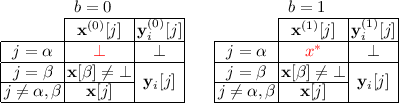
• - Query Phase I: The attacker adaptively queries the challenger for private keys corresponding to attribute vectors pairs $\mathbf{y}_{i}^{(0)},\mathbf{y}_{i}^{(1)}\in \{\{0,1\}^n\cup \bot \}^d$ for $i=1,...,q_1$. The challenger responds with the secret keys for $\mathbf{y}_{i}^{(\beta )}$.

• - Challenge: The attacker declares two message s vector $\mathbf{x}^{(0)}, \mathbf{x}^{(1)}\in \{\{0,1\}^n\cup \bot \}^d$. The challenger responds with the ciphertext $C \leftarrow \mathbf{Encrypt}_S(MSK,\mathbf{x}^{(\beta )})$.

• - Query Phase II: The attacker continues to adaptively queries the challenger for private keys corresponding to attribute vectors pairs $\mathbf{y}_{i}^{(0)},\mathbf{y}_{i}^{(1)}\in \{\{0,1\}^n\cup \bot \}^d$ for $i=q_1+1,...,q$. The challenger responds with the secret keys for $\mathbf{y}_{i}^{(\beta )}$.

• - Guess: The attacker outputs a guess $\beta '$ for $\beta$.

• - Check: The challenger evaluates a predicate P on the secret-key and challenge queries: $c=P(\{\mathbf{y}_{i}^{(b)}\}_{i\in [q],b\in \{0,1\}},\mathbf{x}^{(0)}, \mathbf{x}^{(1)})$. If the predicate holds ($c=1$) then the challenger outputs $\beta '' = \beta '$. Otherwise the challenger outputs a random independent bit $\beta ''$.

The advantage of an attacker in this game is defined to be $\Pr [\beta = \beta '']- \frac{1}{2}$ (and note that if $c=0$ then the advantage is 0). The scheme is secure relative to the given predicate if feasible adversaries can only have a negligible advantage.

The predicate P. The security game varies depending on the predicate P, with more permissive predicates yielding stronger notions of security. At a minimum, we need P to exclude queries that let the adversary trivially distinguish the left and right sides by applying the decryption procedure on the secret keys and ciphertext received. Similarly, P must also exclude queries that let the adversary distinguish the left and right sides by generating its own ciphertexts.

However, it is not hard to see that using a permissive predicate P that only excludes these trivial attacks results in a security notion that is too strong: such permissive P would allow arbitrary secret-key queries $(y,y')$ so long as $\mathsf {C}(x,y)=\mathsf {C}(x,y')$ for all $x\in \{0,1\}^n$, which means that we directly get indistinguishability obfuscation. Specifically, for a universal circuit U, we obfuscate a function $f(x)=U(f,x)$ by publishing the FE secret key $SK_f$. This lets anyone evaluate f(x) for any x by encrypting x under the scheme, and then using $SK_f$ to decrypt f(x), and the security notion would say that any two functionally equivalent f and $f'$ are indistinguishable.

Next, we therefore describe some simple predicates which are more restrictive, and hence they correspond to weaker notions of security (which are still strong enough for our purposes). Very roughly speaking, they all require that most of the time we have $\mathbf{y}_{i}^{(0)}=\mathbf{y}_{i}^{(1)}$ and/or $\mathbf{x}^{(0)}=\mathbf{x}^{(1)}$, and they differ only in a handful of slots and/or a handful of queries.

4.1 Core Predicates

We begin by describing some simple core predicates that our slotted FE scheme should satisfy. In the next section we show that the corresponding security properties imply also stronger properties, including adaptively security of the induced unslotted FE scheme.

• 0. Slot Symmetry. P checks that there are two distinct non-special slots $\alpha \ne \beta$, $\alpha ,\beta \ne 0$ such that:

  • $\mathbf{x}^{(0)}, \mathbf{x}^{(1)}$ are equal in all the slots other than $\alpha ,\beta$, and they swap the content of these two slots. Namely $\mathbf{x}^{(0)}[j]=\mathbf{x}^{(1)}[j]:=\mathbf{x}[j]$ for all $j\notin \{\alpha ,\beta \}$, and $\mathbf{x}^{(b)}[\alpha ]=\mathbf{x}^{(1-b)}[\beta ]:=x^{(b*)}$ for $b=0,1$.

  • Similarly for all i $\mathbf{y}_i^{(0)}, \mathbf{y}_i^{(1)}$ are equal in all the slots other than $\alpha ,\beta$, and they swap the content of these two slots. Namely $\mathbf{y}_i^{(0)}[j]=\mathbf{y}_i^{(1)}[j]:=\mathbf{y}_i[j]$ for all $j\notin \{\alpha ,\beta \}$, and $\mathbf{y}_i^{(b)}[\alpha ]=\mathbf{y}_i^{(1-b)}[\beta ]:=y_i^{(b*)}$ for $b=0,1$.

    

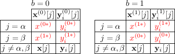
  Intuitively, this allows us to permute the contents of different slots without the adversary’s notice.

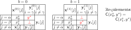
• 1. Single-Use Message and Function Hiding. P checks that there is a non-special slot $\alpha \ne 0$ and a secret key query $\gamma \in [q]$ such that:

  • All key-queries other than $\gamma$ contain two identical functions, $\mathbf{y}_i^{(0)}=\mathbf{y}_i^{(1)}:=\mathbf{y}_i$ $\forall i\ne \gamma$.

  • Key-query $\gamma$ has two keys that differ only in slot $\alpha$, $\mathbf{y}_\gamma ^{(0)}[j]=\mathbf{y}_\gamma ^{(1)}[j]:=\mathbf{y}_\gamma [j]$ $\forall j\ne \alpha$.

  • The challenge query has two plaintexts that differ only in slot $\alpha$, $\mathbf{x}^{(0)}[j]=\mathbf{x}^{(1)}[j]:=\mathbf{x}[j]$ $\forall j\ne \alpha$.

  • We have either the same functionality $\mathsf {C}(\mathbf{x}^{(0)}[\alpha ],\mathbf{y}_\gamma ^{(0)}[\alpha ])=\mathsf {C}(\mathbf{x}^{(1)}[\alpha ],{} \mathbf{y}^{(1)}[\alpha ])$, or the two plaintext slots are inactive $\mathbf{x}^{(0)}[\alpha ]=\mathbf{x}^{(1)}[\alpha ]=\bot$, or the two key slots are inactive $\mathbf{y}^{(0)}_\gamma [\alpha ]=\mathbf{y}^{(1)}_\gamma [\alpha ]=\bot$.

    

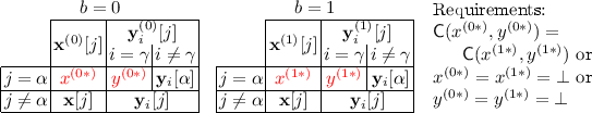
  This allows us to argue both message and function hiding for one slot in one query, as long as that slot is not the special slot that the public parameters can encrypt to.

• 2. Slot Duplication. P checks that there are distinct slots $\alpha \ne \beta$ with $\beta \ne 0$ such that:

  • All the slots other than $\beta$ are the same between left and right, $\mathbf{x}^{(0)}[j]=\mathbf{x}^{(1)}[j]:=\mathbf{x}[j]$ for all $j\ne \beta$, and $\mathbf{y}_i^{(0)}[j]=\mathbf{y}_i^{(1)}[j]:=\mathbf{y}_i[j]$ for all i and all $j\ne \beta$.

  • Slots $\beta$ on the left are inactive, $\mathbf{x}^{(0)}[\beta ]=\bot$ and $\mathbf{y}^{(0)}_i[\beta ]=\bot$ for all i

  • Slots $\beta$ on the right are either inactive or equal to slots $\alpha$, $\mathbf{x}^{(0)}[\beta ]\in \{\mathbf{x}[\alpha ],\bot \}$ and $\mathbf{y}^{(0)}_i[\beta ]\in \{\mathbf{y}_i[\alpha ],\bot \}$ for all i.

    

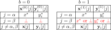
  We stress that slot duplication can duplicate the slots of the ciphertext and secret keys simultaneously. We can choose to duplicate the slots of all keys and the ciphertext, or any subset of them.

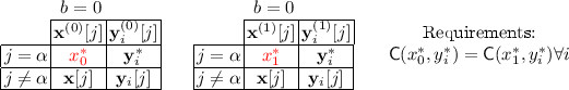
• 3. Ciphertext Moving. P checks that there are two distinct slots $\alpha \ne \beta$ such that:

  • For each secret key, all slots (including $\alpha$ and $\beta$) are the same on the left and right: $\mathbf{y}^{(0)}_i[j]=\mathbf{y}^{(1)}_i[j]:=\mathbf{y}_i[j]$ for all i and j.

  • For each secret key, slot $\alpha$ is identical to slot $\beta$ on both the left and right: $\mathbf{y}_i[\alpha ]=\mathbf{y}_i[\beta ]:=\mathbf{y}_i^*$ ($\mathbf{y}_i^*$ is potentially $\bot$).

  • For the challenge ciphertext, all slots other than $\alpha ,\beta$ are the same between left and right: $\mathbf{x}^{(0)}[j]=\mathbf{x}^{(1)}[j]:=\mathbf{x}[j]$ for all $j\notin \{\alpha ,\beta \}$.

  • For the challenge ciphertext, slot $\beta$ on the left and slot $\alpha$ on the right are inactive: $\mathbf{x}^{(0)}[\beta ]=\mathbf{x}^{(1)}[\alpha ]=\bot$.

  • For the challenge ciphertext, slot $\alpha$ on the left is equal to slot $\beta$ on the right: $\mathbf{x}^{(0)}[\alpha ]=\mathbf{x}^{(1)}[\beta ]=\mathbf{x}^*$.

    

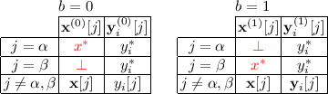
  This lets us rearrange the slots of the challenge ciphertext, as long as each secret keys is identical among the affected slots. We stress that ciphertext moving allows one of the slots being rearranged to be the special slot.

• 4. Weak key moving. P checks that there are two distinct non-special slots $\alpha \ne \beta$, $\alpha ,\beta \ne 0$ and secret-key query $\gamma$ such that:

  • For the challenge ciphertext, all slots (including $\alpha$ and $\beta$) are the same between left and right: $\mathbf{x}^{(0)}[j]=\mathbf{x}^{(1)}[j]:=\mathbf{x}[j]$ for all j.

  • For the challenge ciphertext, slot $\alpha$ is identical to slot $\beta$ on both the left and right: $\mathbf{x}[\alpha ]=\mathbf{x}[\beta ]:=x^*$

  • For each secret key query other than $\gamma$, all slots (including $\alpha$ and $\beta$) are the same on the left and right: $\mathbf{y}^{(0)}_i[j]=\mathbf{y}^{(1)}_i[j]:=\mathbf{y}_i[j]$ for all $i\ne \gamma$ and all j.

  • For secret key query $\gamma$, all slots other than $\alpha ,\beta$ are the same on the left and right: $\mathbf{y}^{(0)}_\gamma [j]=\mathbf{y}^{(1)}_\gamma [j]:=\mathbf{y}_\gamma [j]$ for all $j\notin \{\alpha ,\beta \}$.

  • For secret key query $\gamma$, slot $\beta$ on the left and slot $\alpha$ on the right are inactive: $\mathbf{y}^{(0)}_\gamma [\beta ]=\mathbf{y}^{(1)}_\gamma [\alpha ]=\bot$.

  • For secret key query $\gamma$, slot $\alpha$ on the left is identical to slot $\beta$ on the right: $\mathbf{y}^{(0)}_\gamma [\alpha ]=\mathbf{y}^{(1)}_\gamma [\beta ]=\mathbf{y}_\gamma ^*:=y^*$.

    

  This is the secret key version of ciphertext moving, allowing us to rearrange the slots of a secret key, as long as the challenge ciphertext is identical among the affected slots. The main difference from ciphertext moving is that weak key moving does not allow us to modify the special slot 0.

We observe that the above properties, even in combination, will never allow the changing of a secret key in slot 0. Thus, we will not be able to obtain any form of function hiding for the derived unslotted functional encryption scheme just from the properties above. This serves as a sanity check that the above properties are not too strong, and might be obtainable from simple assumptions, and indeed we give a construction meeting these in Sect. 5.

In the following sections, we present several other more complex predicates, and show that security relative to the complex predicates is implied by the security relative only to the predicates above. The proofs “consume” some slots, so extra slots are needed to obtain security for the more complex predicates.

One of the predicates we prove security for corresponds exactly to regular functional encryption. The total number of slots consumed in the proof from the basic predicates is 3. Combining with our slotted FE construction in Sect. 5 for 4 slots, we obtain adaptively secure functional encryption for $NC^1$ functionalities.

In the full version [GGHZ14b], we show how to use our predicates, together with puncturable PRFs and randomized encodings (defined in Sect. 3) to obtain functional encryption for all circuits. The total number of slots consumed is 5, meaning we need a 6-slotted FE. In particular, the number of slots is constant, which translates to a constant number (namely 6) of subgroups in the underlying composite-order multilinear maps.

4.2 Additional Derivable Predicates

Now we describe several additional properties that can be derived from the core properties above, potentially “using up” several additional slots.

• 5. New Slot. P checks that there are distinct slots $\alpha \ne \beta$ with $\alpha$ not being the special 0 slot (but $\beta$ may be), such that:

  • For each secret key, all slots (including $\alpha$ and $\beta$) are the same on the left and right: $\mathbf{y}^{(0)}_i[j]=\mathbf{y}^{(1)}_i[j]$ for all i and j.

  • For each secret key, slot $\alpha$ is inactive on both the left and the right: $\mathbf{y}^{(0)}_i[\alpha ]=\mathbf{y}^{(1)}_i[\alpha ]=\bot$ for all i

  • For the challenge ciphertext, all slots other than slot $\alpha$ are the same on the left and right: $\mathbf{x}^{(0)}[j]=\mathbf{x}^{(1)}[j]$ for all $j\ne \alpha$.

  • For the challenge ciphertext, slot $\beta$ is active on both the left and the right: $\mathbf{x}^{(0)}[\beta ]=\mathbf{x}^{(1)}[\beta ]\ne \bot$.

  • For the challenge ciphertext, slot $\alpha$ is inactive on the left: $\mathbf{x}^{(0)}[\alpha ]=\bot$

    

  Notice that there is no restriction to the value in slot $\alpha$ of the ciphertext on the right. Thus, the allows us to take a slot that is inactive for all secret keys and the challenge ciphertext, and place an arbitrary value in the slot for the ciphertext.

• 6. Strong key moving. P checks that there are distinct non-special slots $\alpha \ne \beta$, $\alpha ,\beta \ne 0$, and secret key query $\gamma$ such that:

  • For the challenge ciphertext, all slots (including $\alpha$ and $\beta$) are the same between left and right: $\mathbf{x}^{(0)}[j]=\mathbf{x}^{(1)}[j]:=\mathbf{x}[j]$ for all j.

  • For each secret key query other than $\gamma$, all slots (including $\alpha$ and $\beta$) are the same on the left and right: $\mathbf{y}^{(0)}_i[j]=\mathbf{y}^{(1)}_i[j]:=\mathbf{y}_i[j]$ for all $i\ne \gamma$ and all j.

  • For secret key query $\gamma$, all slots other than $\alpha ,\beta$ are the same on the left and right: $\mathbf{y}^{(0)}_\gamma [j]=\mathbf{y}^{(1)}_\gamma [j]:=\mathbf{y}_\gamma [j]$ for all $j\notin \{\alpha ,\beta \}$.

  • For secret key query $\gamma$, slot $\beta$ on the left and slot $\alpha$ on the right are inactive: $\mathbf{y}^{(0)}_\gamma [\beta ]=\mathbf{y}^{(1)}_\gamma [\alpha ]=\bot$.

  • For secret key query $\gamma$, slot $\alpha$ on the left is identical to slot $\beta$ on the right: $\mathbf{y}^{(0)}_\gamma [\alpha ]=\mathbf{y}^{(1)}_\gamma [\beta ]:=\mathbf{y}_\gamma ^*$.

  • When decrypting the challenge with secret key $\gamma$, slot $\alpha$ on the left and slot $\beta$ on the right give the same result. In other words, $\mathsf {C}(\mathbf{x}[\alpha ],\mathbf{y}_\gamma ^*)=\mathsf {C}(\mathbf{x}[\beta ],\mathbf{y}_\gamma ^*)$

    

  This is a stronger form of secret key moving where we can actually rearrange secret key slots even if the challenge ciphertext differs in those slots, as long as decryption is unaffected.

• 7. Weak ciphertext indistinguishability. P checks that there is a non-special slot $\alpha \ne 0$ such that:

  • For each secret key, all slots (including slot $\alpha$) are the same on the left and right: $\mathbf{y}^{(0)}_i[j]=\mathbf{y}^{(1)}_i[j]:=\mathbf{y}_i[j]$ for all i and j.

  • For the challenge ciphertext, all slots except slot $\alpha$ are the same on the left and right: $\mathbf{x}^{(0)}_i[j]=\mathbf{x}^{(1)}_i[j]:=\mathbf{x}[j]$ for all $j\ne \alpha$.

  • For the challenge ciphertext, slot $\alpha$ decrypts to the same result for each secret key query: $\mathsf {C}(\mathbf{x}^{(0)}[\alpha ],\mathbf{y}_i[\alpha ])=\mathsf {C}(\mathbf{x}^{(1)}[\alpha ],\mathbf{y}_i[\alpha ])$.

    

  In other words, we can change the value of the ciphertext in any slot other than the special 0 slot as long as decryption is unaffected. This almost gives us functional encryption, except for the requirement that the slot is not the special slot.

• 8. Strong ciphertext indistinguishability. Same as above, except $\alpha$ can be 0.

4.3 Reductions

Now we describe several reductions showing that core properties described above are sufficient for obtaining the additional derivable properties also described above, at the cost of “using up” several additional slots. We note that in all of the reductions below, any existing property, whether core or derived, is preserved in the reduction.

Lemma 3

(1) Single-use hiding and (2) slot duplication imply (5) new slot.

Proof

Use slot duplication to duplicate contents of the $\beta$ slot into the originally empty $\alpha$ slot of the ciphertext (don’t duplicate the secret keys), and then use single-use message and function hiding to change the message to $x^*$, which is possible since there are no secret keys components in the $\alpha$ slot.

Lemma 4

(1) Single-use hiding, (2) slot duplication, (3) and weak key moving for $d+1$ slots implies (6) strong key moving for d slots (all existing properties being preserved).

Proof

We prove for $\alpha =1,\beta =2$, the other cases being identical. We will move secret key $\gamma \in [q]$. Let slot $d+1$ be a “scratch” slot, that is unused by the normal scheme. We will use slot $d+1$ in the security proof. Below is the table of hybrids. For secret keys $i \in [q], i \ne \gamma$ not included in the table, slot $d+1$ is inactive, and the rest of the slots remain the same throughout all hybrids. Similarly, slots $j\ne 1,2,d+1$ remain the same for the ciphertext and the $\gamma$th secret key.

Lemma 5

(0) Slot symmetry, (5) new slot, and (6) strong key moving for $d+1$ slots implies weak (7) weak ciphertext indistinguishability for d slots (all existing properties being preserved).

Proof

We prove for $\alpha =1$, the other cases being identical. The slot $d+1$ will be the “scratch” slot, that is unused by the normal scheme but used in the security proof. In the hybrids below we will use the strong key moving property. Note that the strong key moving only allows for changing one key at a time, while in the hybrids below we will need to change all the keys. This can be done by changing one key at a time.

Lemma 6

(2) Slot duplication, (3) weak ciphertext moving, and (7) weak ciphertext indistinguishability for $d+1$ slots implies (8) strong ciphertext indistinguishability for d slots (all existing properties preserved).

Proof

Only need to add the case for slot 0. Just as before, the slot $d+1$ will be the “scratch” slot, that is unused by the normal scheme but used in the security proof.

5 Slotted Functional Encryption for $NC^1$

We now give our slotted FE scheme for $NC^1$. We will describe our scheme in terms of matrix branching programs, using Barrington’s Theorem (Theorem 2) to realize slotted FE for $NC^1$ circuits. We describe our scheme for single bit outputs — it can easily be extended to multi-bit outputs by running multiple instances of the scheme in parallel.

Setup $(\lambda , BP,d)$: Given a universal 2-input matrix branching program

$$\begin{aligned} BP=\left( {\mathsf {bit}},{\mathsf {inp}},\left( B_{i,b}\right) _{i\in [\ell ],b\in \{0,1\}}\right) \end{aligned}$$

run $\mathsf {params}\leftarrow \mathsf {InstGen}(1^\lambda ,\{1,\dots ,\ell \},d)$. Then, choose random matrices $R_i\in \mathfrak {R}$ for $i\in [\ell -1]$, as well as random $\alpha _{i,b}$ for $i\in [\ell ],b\in \{0,1\}$. Let $\tilde{B}_{i,b}=\alpha _{i,b}\cdot R_{i-1}\cdot B_{i,b}\cdot R_i^{-1}$ for $i\in [2,\ell -1]$, and $\tilde{B}_{1,b}=\alpha _{1,b}\cdot B_{1,b}\cdot R_1^{-1}$ and $\tilde{B}_{\ell ,b}=\alpha _{\ell ,b}\cdot R_{\ell -1}\cdot B_{\ell ,b}$ ⁶. Compute $A_{i,b}^j=[\tilde{B}_{i,b}]^{j}_{\{i\}}$ for $j\in [d]$. (Here $R_0$ and $R_\ell$ are set to identity.)

Let $\mathbb {V}$ be the subset of $[\ell ]$ that corresponds to the secret key: $\mathbb {V}=\{i\in [\ell ]:{\mathsf {inp}}(i)=0\}$, and $\mathbb {W}$ be the subset of $[\ell ]$ that corresponds to the ciphertext: $\mathbb {W}=\{i\in [\ell ]:{\mathsf {inp}}(i)=1\}$. Then the universe $\mathbb {U}=\mathbb {V}\cup \mathbb {W}$.

The master public key is $MPK=(\mathsf {params},(A_{i,b}^0)_{i\in \mathbb {W},b\in \{0,1\}})$

The master secret key consists of the $A_{i,b}^j$ for $i\in \mathbb {V}\cup \mathbb {W}$.

KeyGen $_S(MSK,\mathbf{y})$: Given an attribute $y\in \{\{0,1\}^n\cup \bot \}^d$, choose random $\beta _{i}\in \mathfrak {R}$ for $i\in \mathbb {V},b\in \{0,1\}$, and output the secret key

$$\begin{aligned} SK_y={\mathsf {extend}}\left( \mathsf {params},\mathbb {V},\left( \beta _i \cdot \left( \sum _{j:y[j]\ne \bot }A^j_{i,y[j]_{{\mathsf {bit}}(i)}}\right) \right) _{i\in \mathbb {V}}\;\;\right) \end{aligned}$$

Encrypt $_S(MSK,\mathbf{x})$: Given an attribute $x\in \{\{0,1\}^n\cup \bot \}^d$, choose random $\beta _{i}\in \mathfrak {R}$ for $i\in \mathbb {W},b\in \{0,1\}$, and output the ciphertext

$$\begin{aligned} C={\mathsf {extend}}\left( \mathsf {params},\mathbb {W},\left( \beta _i \cdot \left( \sum _{j:x[j]\ne \bot }A^j_{i,x[j]_{{\mathsf {bit}}(i)}}\right) \right) _{i\in \mathbb {W}}\;\;\right) \end{aligned}$$

Encrypt(MPK, m): Given a message $m\in \{0,1\}^n$, choose random $\beta _i\in \mathfrak {R}$ for $i\in \mathbb {W}$, and output the ciphertext

$$\begin{aligned} C={\mathsf {extend}}\left( \mathsf {params},\mathbb {W},\left( \beta _i\cdot A^0_{i,m_{{\mathsf {bit}}(i)}}\right) _{i\in \mathbb {W}}\;\;\right) \end{aligned}$$

Remark 3

Note that all the encodings given out in the ciphertext can be re-randomized (to noise $\sigma '$) using the randomizer provided in the public parameters. We do not mention the re-randomization above explicitly, for the sake of simplicity of notation.

Decrypt(MPK, SK, C): Given a secret key $SK=f_{\mathbb {V}'\rightarrow \mathbb {V}}, (K_i)_{i\in \mathbb {V}'}$ and a ciphertext $C=f_{\mathbb {W}'\rightarrow \mathbb {W}}, (C_i)_{i\in \mathbb {W}'}$, let $D_i={\left\{ \begin{array}{ll}K_i&{}\text {if }i\in \mathbb {V}'\\ C_i&{}\text {if }i\in \mathbb {W}'\end{array}\right. }$, and compute the product

$$\begin{aligned} D=f_{\mathbb {V}'\rightarrow \mathbb {V}}\left( f_{\mathbb {W}'\rightarrow \mathbb {W}}\left( \prod _{i\in \mathbb {U}}D_i\right) \right) \end{aligned}$$

Then run the zero-test procedure on a distinguishing coordinate of D.

Correctness. Evaluation is carried out slot by slot. In slot j, if either K or C is inactive, then the corresponding ring will be empty. Therefore, the result of the computation is 0 in slot j. In a slot j where K and C are both active, then write $K_i[j]=[\beta _i \alpha _{i,y[j]_{{\mathsf {bit}}(i)}} \tilde{B}_{i,y_{{\mathsf {bit}}(i)}}]^j_{\{i'\}}$ and $C_i[j]=[\beta _i \alpha _{i,m_{{\mathsf {bit}}(i)}} \tilde{B}_{i,m_{{\mathsf {bit}}(i)}}]^j_{\{i'\}}$ for some index elements $i'$ to be the components of K, C in the ring $\mathfrak {R}_j$. Let $d[j]=(y[j],m[j])\in \{0,1\}^{2n}$. Then we can write $D_i[j]=[\beta _i\alpha _{i,d[j]_{{\mathsf {inp}}(i),{\mathsf {bit}}(i)}}\tilde{B}_{i,d[j]_{{\mathsf {inp}}(i),{\mathsf {bit}}(i)}}]^j_{\{i\}}$.

Therefore, the product $D'[j]=\prod _{i\in \mathbb {U}}D_i[j]$ is equal to

$$\begin{aligned}D'[j]&=\left[ \prod _{i\in \mathbb {U}}\left( \beta _i\alpha _{i,d[j]_{{\mathsf {inp}}(i),{\mathsf {bit}}(i)}}\right) \prod _{i\in \mathbb {U}}\tilde{B}_{i,d[j]_{{\mathsf {inp}}(i),{\mathsf {bit}}(i)}}\right] ^j_{\mathbb {U}'}\\ {}&=\left[ \prod _{i\in \mathbb {U}}\left( \beta _i\alpha _{i,d[j]_{{\mathsf {inp}}(i),{\mathsf {bit}}(i)}}\right) \prod _{i\in \mathbb {U}}B_{i,d[j]_{{\mathsf {inp}}(i),{\mathsf {bit}}(i)}}\right] ^j_{\mathbb {U}'}\end{aligned}$$

where $\mathbb {U}'=\mathbb {V}'\cup \mathbb {W}'$. Applying $f_{\mathbb {W}'\rightarrow \mathbb {W}}$ to this encoding gives an encoding of the same product, but relative to the set $\mathbb {V}'\cup \mathbb {W}$, and then applying $f_{\mathbb {V}'\rightarrow \mathbb {V}}$ gives the encoding relative to $\mathbb {U}$. Therefore, $D=f_{\mathbb {V}'\rightarrow \mathbb {V}}(f_{\mathbb {W}'\rightarrow \mathbb {W}}(D'))$ satisfies

$$\begin{aligned}D[j]&=\left[ \prod _{i\in \mathbb {U}}\left( \beta _i\alpha _{i,d[j]_{{\mathsf {inp}}(i),{\mathsf {bit}}(i)}}\right) \prod _{i\in \mathbb {U}}B_{i,d[j]_{{\mathsf {inp}}(i),{\mathsf {bit}}(i)}}\right] ^j_{\mathbb {U}}\\ {}&=\left[ \prod _{i\in \mathbb {U}}\left( \beta _i\alpha _{i,d[j]_{{\mathsf {inp}}(i),{\mathsf {bit}}(i)}}\right) M_{BP(d[j])}\right] ^j_{\mathbb {U}}\end{aligned}$$

We only care about ciphertexts and secret keys where the branching program evaluates the same in every slot, so BP(d[j]) is the same for all active slots j; call the result b. Define $\gamma [j]=\beta _i\alpha _{i,d[j]_{{\mathsf {inp}}(i),{\mathsf {bit}}(i)}}$ projected down to ring $\mathfrak {R}_j$, and $\gamma =\sum _{j\in S}\gamma [j]$ where S is the set of active slots. Note that we only care about secret keys and ciphertext where there is at least one active slot. Therefore with overwhelming probability $\gamma \ne 0$.

We can now write $D = \left[ \gamma M_b\right] _{\mathbb {U}}$. Then when we zero test a distinguishing coordinate of D, with overwhelming probability, the result will match b.

5.1 Security Proof

Theorem 4

Assuming Assumptions 1 and 2, the scheme described above satisfies the core properties of the slotted FE scheme.

Slot Symmetry. Our scheme satisfies perfect slot symmetry, where the advantage of an even infinitely powerful adversary is 0. This follows from the fact that slots correspond to sub-rings in our scheme, and our subrings are generated in a totally symmetric manner.

Single-use Message and Function hiding. In our scheme, the matrices are just the matrices from Kilian-randomized branching programs, where the randomization in each sub-ring is independent. In the single slot j where changes are made, only the ciphertext and a single public key are active. Let $z=(x_0,y_0)$ be the ciphertext and secret key values active on the left side, and $z'=(x_1,y_1)$ be the values on the right side. Then on the left side, only the matrices $\tilde{B}_{i,z[{\mathsf {inp}}(i)]_{{\mathsf {bit}}(i)}}$ are handed out in ring $\mathfrak {R}_j$, and by Theorem 3, these matrices are uniform random matrices subject to their product being $M_{\mathsf {C}(x_0,y_0)}$. Similarly, on the left size, the matrices handed out are uniform random matrices subject their product being $M_{\mathsf {C}(x_1,y_1)}$. Since $\mathsf {C}(x_0,y_0)=\mathsf {C}(x_1,y_1)$, these distributions are identical, so our scheme satisfies perfect single use hiding.

Slot duplication. We will prove slot duplication from Assumption 1. Let $\alpha \in [d]$ and $\beta \ne \alpha ,0$. Obtain the challenge for assumption 1, and re-order the rings so that the challenge has the form $\left( S_{i,j}=[s_{i,j}]^j_{\{i\}}\right) _{i\in \mathbb {U},j\ne \beta }\!,\left( T_i\right) _{i\in \mathbb {U}}$ where $T_i=[t_i]^{\alpha }_{\{i\}}$ or $T_i=[t_i]^{\alpha ,\beta }_{\{i\}}$. We now simulate the view of the adversary as follows. Given a 0/1 matrix B and an encoding e, let $e\cdot B$ be the matrix of encodings, where $e\cdot B$ has e in any position where B has a 1, and an encoding of 0 in any position where B has a 0 (note that we will be multipling $e\cdot B$ by other matrices of encodings, so the encodings of 0 do not actually have to be computed, but merely serve as placeholders in the computation).

Choose random matrices $R_i\in \mathfrak {R}$ for $i\in [\ell -1]$, as well as random $\alpha '_{i,b}$, and set $A^j_{i,b}=\alpha '_{i,b}\cdot R_{i-1}\cdot (S_{i,j}\cdot B_{i,b})\cdot R_i^{-1}$ for $j\ne \beta$ ⁷. This formally sets $\alpha _{i,b}=\alpha '_{i,b}s_{i,j}$ in ring $\mathfrak {R}_j$, which leaves $\alpha _{i,b}$ in ring $\beta$ undetermined. Define $D^j_{i,b}=\alpha '_{i,b}\cdot R_{i-1}\cdot (T_i\cdot B_{i,b})\cdot R_i^{-1}$.

Using the $A_{i,b}^j$, we can simulate the public paramters as in the scheme. To answer the challenge ciphertext query, there are two cases. If slot $\beta$ is empty, then we can answer the challenge ciphertext query as in the slotted FE scheme with the $A_{i,b}^j$ (since $\beta$ is empty, we do not need $A_{i,b}^\beta$). If slot $\beta$ is not a copy of slot $\alpha$ on either side of the challenge, then we answer the challenge query by choosing a random $\beta '_{i}\in \mathfrak {R}$ for $i\in \mathbb {W},b\in \{0,1\}$, and output the ciphertext

$$\begin{aligned} C={\mathsf {extend}}\left( \mathsf {params},\mathbb {W},\left( \beta '_i \cdot \left( \sum _{j:x[j]\ne \bot ,j\notin \{\alpha ,\beta \}}A^j_{i,x[j]_{{\mathsf {bit}}(i)}}+D^j_{i,x[\alpha ]_{{\mathsf {bit}}(i)}}\right) \right) _{i\in \mathbb {W}}\;\;\right) \end{aligned}$$

If the $T_i$ are only encodings in ring $\mathfrak {R}_\alpha$, then this correctly simulates the ciphertext when slot $\beta$ empty, formally setting $\beta _i=\beta _i$ in rings other that $\mathfrak {R}_\alpha ,\mathfrak {R}_\beta$, and setting $\beta _i=\beta '_i t_i$ in rings $\mathfrak {R}_\alpha ,\mathfrak {R}_\beta$ (the value in $\mathfrak {R}_\beta$ is irrelevant in this case). If the $T_i$ are encodings in $\mathfrak {R}_\alpha \times \mathfrak {R}_\beta$, then this correctly simulates the ciphertext when slot $\beta$ is a copy of slot $\alpha$, with the same formal settings of variables as before.

We can perform a similar procedure to simulate the secret key queries. In the end, if $T_i$ are only encodings in $\mathfrak {R}_\alpha$, then this correctly simulates the left side in slot duplication, where slot $\beta$ is empty. If $T_i$ are encodings in $\mathfrak {R}_\alpha \times \mathfrak {R}_\beta$, then this correctly simulates the right side of slot duplication, where slot $\beta$ is sometimes a copy of slot $\alpha$. Thus, if Assumption 1 holds, the two cases are indistinguishable.

Ciphertext moving. We will prove ciphertext moving from Assumption 2. Let $\alpha \ne \beta$, where $\alpha$ is the slot the ciphertext is in, and $\beta$ is the slot we wish to move the ciphertext to. Obtain the challenge for assumption 2, and re-order the rings so that the challenge has the form

$$\begin{aligned}&\left( S_{i,j}=[s_{i,j}]^j_{\{i\}}\right) _{i\in \mathbb {V},j\notin \{\alpha ,\beta \}},\left( S_{i,j}=[s_{i,j}]^j_{\{i\}}\right) _{i\in \mathbb {W},j\in [d]},\left( T_i=[t_i]^{\alpha ,\beta }_{\{i\}}\right) _{i\in \mathbb {V}},\\&E={\mathsf {extend}}^\dagger \left( \mathsf {params},\mathbb {W},\left\{ \left( U_{i,j}=[u_{i,j}]^j_{\{i\}}\right) _{i\in \mathbb {W},j>1},\left( V_i=[v_i]^{\gamma }_{\{i\}}\right) _{i\in \mathbb {W}}\right\} \;\;\right) \end{aligned}$$

where $\gamma =\alpha$ or $\gamma =\beta$.

We now simulate the view of the adversary. Choose random matrices $R_i\in \mathfrak {R}$ for $i\in [\ell -1]$, random $\alpha '_{i,b}$, and set $A^j_{i,b}=\alpha '_{i,b}\cdot R_{i-1}\cdot (S_{i,j}\cdot B_{i,b})\cdot R_i^{-1}$ for $i\in \mathbb {V}$, $j\notin \{\alpha ,\beta \}$, and all $i\in \mathbb {W}$, $j\in [d]$. This formally sets $\alpha _{i,b}=\alpha '_{i,b}s_{i,j}$ in ring $\mathfrak {R}_j$, which leaves $\alpha _{i,b}$ in rings $\alpha$ and $\beta$ undetermined for $i\in \mathbb {V}$. Define $A^{\alpha }_{i,b}+A^{\beta }_{i,b}=\alpha '_{i,b}\cdot R_{i-1}\cdot (T_{i}\cdot B_{i,b})\cdot R_i^{-1}$ for $i\in \mathbb {V}$, which formally sets $\alpha _{i,b}=\alpha '_{i,b}T_i$ in rings $\mathfrak {R}_\alpha$ and $\mathfrak {R}_\beta$.

Now using the $A_{i,b}^j$ values, we can simulate the public parameters (since we have all the values for $i\in \mathbb {W},j=0$), as well as all the secret key queries (since all the secret key queries are identical in slots $\alpha$ and $\beta$, meaning we will always have $A^{\alpha }_{i,b}+A^{\beta }_{i,b}$ together, neither being used separately). To generate the challenge ciphertext, we use the result E of extension. Let $U'_{i,j}$ be the components in E corresponding to the $U_{i,j}$, and $V'_i$ the components corresponding to the $V_i$. Then the challenge ciphertext is set as

$$\begin{aligned}C=&f_{\mathbb {W}'\rightarrow \mathbb {W}},\\ {}&\left( \beta _i\cdot R_{i-1}\cdot \left( (V'_i \cdot B_{i,x^*_{{\mathsf {bit}}(i)}})+\sum _{j:x[j]\ne \bot ,j\notin \{\alpha ,\beta \}}(U'_{i,j}\cdot B_{i,x[j]_{{\mathsf {bit}}(i)}})\right) \cdot R_i^{-1}\right) _{i\in \mathbb {W}}\end{aligned}$$

Note that the randomization terms given in E must be used to randomize the components above.

Where $x^*$ is the ciphertext term that is either in slot $\alpha$ or slot $\beta$. It is straightforward to show that if the $V_i$ are encodings in $\mathfrak {R}_\alpha$, then this simulates the challenge ciphertext with $x^*$ in slot $\alpha$, and similarly if $V_i$ are encodings in $\mathfrak {R}_\beta$, the challenge ciphertext has $x^*$ in slot $\beta$. Therefore, the two cases are indistinguishable and ciphertext moving follows.

Weak key moving. This is basically the same as ciphertext moving, except that we swap the roles of $\mathbb {W}$ and $\mathbb {V}$. The main difference is that, because now the public parameters lie in $\mathbb {V}$, and we are not given terms in $\mathbb {V}$ containing $\alpha$ separate from $\beta$, we must have $\alpha ,\beta \ne 0$ so that we can still generate the public parameters in $\mathfrak {R}_0$.

5.2 Adaptively Secure FE for $NC^1$

Our slotted FE scheme easily gives adaptively secure FE for $NC^1$:

Theorem 5

If assumptions 1 and 2 above hold, then adaptively secure FE for $NC^1$ exists.

Proof

Set $d=4$ in our slotted FE scheme. Then Lemmas 3, 4, 5, and 6 gives a slotted scheme with $d=1$ that satisfies strong ciphertext indistinguishability, which implies adaptive FE security.

References

Ananth, P., Brakerski, Z., Segev, G., Vaikuntanathan, V.: From selective to adaptive security in functional encryption. Cryptology ePrint Archive, Report 2014/917 (2014). http://eprint.iacr.org/2014/917
Agrawal, S., Gorbunov, S., Vaikuntanathan, V., Wee, H.: Functional encryption: new perspectives and lower bounds. In: Canetti, R., Garay, J.A. (eds.) CRYPTO 2013, Part II. LNCS, vol. 8043, pp. 500–518. Springer, Heidelberg (2013)
Ananth, P., Jain, A.: Indistinguishability obfuscation from compact functional encryption. Cryptology ePrint Archive, Report 2015/173 (2015). http://eprint.iacr.org/2015/173
Barrington, D.A.: Bounded-width polynomial-size branching programs recognize exactly those languages in \(nc_1\). In: STOC (1986)
Boyle, E., Goldwasser, S., Ivan, I.: Functional signatures and pseudorandom functions. In: Krawczyk, H. (ed.) PKC 2014. LNCS, vol. 8383, pp. 501–519. Springer, Heidelberg (2014)
Barak, B., Garg, S., Kalai, Y.T., Paneth, O., Sahai, A.: Protecting obfuscation against algebraic attacks. In: Nguyen, P.Q., Oswald, E. (eds.) EUROCRYPT 2014. LNCS, vol. 8441, pp. 221–238. Springer, Heidelberg (2014)
Boneh, D., Lewi, K., Montgomery, H., Raghunathan, A.: Key homomorphic PRFs and their applications. In: Canetti, R., Garay, J.A. (eds.) CRYPTO 2013, Part I. LNCS, vol. 8042, pp. 410–428. Springer, Heidelberg (2013)
Brakerski, Z., Rothblum, G.N.: Virtual black-box obfuscation for all circuits via generic graded encoding. In: Lindell, Y. (ed.) TCC 2014. LNCS, vol. 8349, pp. 1–25. Springer, Heidelberg (2014)
Boneh, D., Silverberg, A.: Applications of multilinear forms to cryptography. Cryptology ePrint Archive, Report 2002/080 (2002). http://eprint.iacr.org/2002/080
Brakerski, Z., Segev, G.: Function-private functional encryption in the private-key setting. In: Dodis, Y., Nielsen, J.B. (eds.) TCC 2015, Part II. LNCS, vol. 9015, pp. 306–324. Springer, Heidelberg (2015)
Boneh, D., Sahai, A., Waters, B.: Functional encryption: definitions and challenges. In: Ishai, Y. (ed.) TCC 2011. LNCS, vol. 6597, pp. 253–273. Springer, Heidelberg (2011)
Bitansky, N., Vaikuntanathan, V.: Indistinguishability obfuscation from functional encryption. Cryptology ePrint Archive, Report 2015/163 (2015). http://eprint.iacr.org/2015/163
Boneh, D., Waters, B.: Constrained pseudorandom functions and their applications. In: Sako, K., Sarkar, P. (eds.) ASIACRYPT 2013, Part II. LNCS, vol. 8270, pp. 280–300. Springer, Heidelberg (2013)
Boneh, D., Wu, D.J., Zimmerman, J.: Immunizing multilinear maps against zeroizing attacks. Cryptology ePrint Archive, Report 2014/930 (2014). http://eprint.iacr.org/2014/930
Boneh, D., Zhandry, M.: Multiparty key exchange, efficient traitor tracing, and more from indistinguishability obfuscation. In: Garay, J.A., Gennaro, R. (eds.) CRYPTO 2014, Part I. LNCS, vol. 8616, pp. 480–499. Springer, Heidelberg (2014)
Coron, J.-S., et al.: Zeroizing without low-level zeroes: New MMAP attacks and their limitations. In: Gennaro, R., Robshaw, M.J.B. (eds.) CRYPTO 2015, Part I. LNCS, vol. 9215, pp. 247–266. Springer, Heidelberg (2015)
Cheon, J.H., Han, K., Lee, C., Ryu, H., Stehlé, D.: Cryptanalysis of the multilinear map over the integers. In: Oswald, E., Fischlin, M. (eds.) EUROCRYPT 2015. LNCS, vol. 9056, pp. 3–12. Springer, Heidelberg (2015)
Coron, J.-S., Lepoint, T., Tibouchi, M.: Practical multilinear maps over the integers. In: Canetti, R., Garay, J.A. (eds.) CRYPTO 2013, Part I. LNCS, vol. 8042, pp. 476–493. Springer, Heidelberg (2013)
Coron, J.-S., Lepoint, T., Tibouchi, M.: New multilinear maps over the integers. Cryptology ePrint Archive, Report 2015/162 (2015). http://eprint.iacr.org/2015/162
Coron, J.-S., Lepoint, T., Tibouchi, M.: New multilinear maps over the integers. In: Gennaro, R., Robshaw, J.B. (eds.) CRYPTO 2015, Part I. LNCS, vol. 9215, pp. 267–286. Springer, Heidelberg (2015)
Gentry, C.: Practical identity-based encryption without random oracles. In: Vaudenay, S. (ed.) EUROCRYPT 2006. LNCS, vol. 4004, pp. 445–464. Springer, Heidelberg (2006)
Garg, S., Gentry, C., Halevi, S.: Candidate multilinear maps from ideal lattices. In: Johansson, T., Nguyen, P.Q. (eds.) EUROCRYPT 2013. LNCS, vol. 7881, pp. 1–17. Springer, Heidelberg (2013)
Garg, S., Gentry, C., Sahai, A., Raykova, M., Sahai, A., Waters, B.: Candidate indistinguishability obfuscation and functional encryption for all circuits. In: 54th Annual Symposium on Foundations of Computer Science, pp. 40–49. IEEE Computer Society Press, Berkeley, CA, USA, 26–29 October 2013
Garg, S., Gentry, C., Sahai, A., Zhandry, M.: Fully secure attribute based encryption from multilinear maps. Cryptology ePrint Archive, Report 2014/622 (2014). http://eprint.iacr.org/2014/622
Garg, S., Gentry, C., Sahai, A., Zhandry, M.: Fully secure functional encryption without obfuscation. Cryptology ePrint Archive, Report 2014/666 (2014). http://eprint.iacr.org/2014/666
Garg, S., Gentry, C., Sahai, A., Waters, B.: Witness encryption and its applications. In: Boneh, D., Roughgarden, T., Feigenbaum, J. (eds.) 45th Annual ACM Symposium on Theory of Computing, pp. 467–476. ACM Press, Palo Alto (2013)
Gentry, C., Lewko, A., Sahai, A., Waters, B.: Indistinguishability obfuscation from the multilinear subgroup elimination assumption. Cryptology ePrint Archive, Report 2014/309 (2014). http://eprint.iacr.org/2014/309
Gentry, C., Lewko, A., Waters, B.: Witness encryption from instance independent assumptions. In: Garay, J.A., Gennaro, R. (eds.) CRYPTO 2014, Part I. LNCS, vol. 8616, pp. 426–443. Springer, Heidelberg (2014)
Gorbunov, S., Vaikuntanathan, V., Wee, H.: Functional encryption with bounded collusions via multi-party computation. In: Safavi-Naini, R., Canetti, R. (eds.) CRYPTO 2012. LNCS, vol. 7417, pp. 162–179. Springer, Heidelberg (2012)
Ishai, Y., Kushilevitz, E.: Randomizing polynomials: a new representation with applications to round-efficient secure computation. In: 41st Annual Symposium on Foundations of Computer Science, pp. 294–304. IEEE Computer Society Press, Redondo Beach, California, USA, 12–14 November 2000
Kilian, J.: Founding cryptography on oblivious transfer. In: 20th Annual ACM Symposium on Theory of Computing, pp. 20–31. ACM Press, Chicago, Illinois, USA, 2–4 May 1988
Kiayias, A., Papadopoulos, S., Triandopoulos, N., Zacharias, T.: Delegatable pseudorandom functions and applications. In: Sadeghi, A.-R., Gligor, V.D., Yung, M. (eds.) ACM CCS 2013: 20th Conference on Computer and Communications Security, pp. 669–684. ACM Press, Berlin (2013)
O’Neill, A.: Definitional issues in functional encryption. Cryptology ePrint Archive, Report 2010/556 (2010). http://eprint.iacr.org/2010/556
Pass, R., Seth, K., Telang, S.: Indistinguishability obfuscation from semantically-secure multilinear encodings. In: Garay, J.A., Gennaro, R. (eds.) CRYPTO 2014, Part I. LNCS, vol. 8616, pp. 500–517. Springer, Heidelberg (2014)
Waters, B.: Efficient identity-based encryption without random oracles. In: Cramer, R. (ed.) EUROCRYPT 2005. LNCS, vol. 3494, pp. 114–127. Springer, Heidelberg (2005)
Waters, B.: Dual system encryption: realizing fully secure ibe and hibe under simple assumptions. In: Halevi, S. (ed.) CRYPTO 2009. LNCS, vol. 5677, pp. 619–636. Springer, Heidelberg (2009)
Waters, B.: A punctured programming approach to adaptively secure functional encryption. Cryptology ePrint Archive, Report 2014/588 (2014). http://eprint.iacr.org/
Yao, A.C.-C.: Protocols for secure computations (extended abstract). In: 23rd Annual Symposium on Foundations of Computer Science, pp. 160–164. IEEE Computer Society Press, Chicago, Illinois, 3–5 November 1982
Author information
Authors and Affiliations
Corresponding author
Editor information
Editors and Affiliations
Rights and permissions
Copyright information
© 2016 International Association for Cryptologic Research
About this paper
Cite this paper
Garg, S., Gentry, C., Halevi, S., Zhandry, M. (2016). Functional Encryption Without Obfuscation. In: Kushilevitz, E., Malkin, T. (eds) Theory of Cryptography. TCC 2016. Lecture Notes in Computer Science(), vol 9563. Springer, Berlin, Heidelberg. https://doi.org/10.1007/978-3-662-49099-0_18
Download citation
DOI: https://doi.org/10.1007/978-3-662-49099-0_18
Published:
Publisher Name: Springer, Berlin, Heidelberg
Print ISBN: 978-3-662-49098-3
Online ISBN: 978-3-662-49099-0
eBook Packages: Computer ScienceComputer Science (R0)