Current Fields of Interest

Abstract

Research in structural optimization started with the onset of structural mechanics. The availability of powerful computers and efficient simulation tools such as FEM, BEM or MBS have led to many optimization methods using closed loops that require no or little user interaction during their implementation. Today, much of the commercial and open source software has more or less integrated the optimization modules, based on various principles. As we can see in many other fields, this possibility did not only result in positive response from the users, but it also increased the demand for easily enabled optimization. We observe an increasing demand for optimization and as a consequence a growing number of tools that help designers to improve on their original ideas.

These keywords were added by machine and not by the authors. This process is experimental and the keywords may be updated as the learning algorithm improves.

Research in structural optimization started with the onset of structural mechanics . The availability of powerful computers and efficient simulation tools such as FEM , BEM or MBS have led to many optimization methods using closed loops that require no or little user interaction during their implementation. Today, much of the commercial and open source software has more or less integrated the optimization modules, based on various principles. As we can see in many other fields, this possibility did not only result in positive response from the users, but it also increased the demand for easily enabled optimization. We observe an increasing demand for optimization and as a consequence a growing number of tools that help designers to improve on their original ideas.

Gradient based optimization and sensitivity studies are common options in CAE-systems today, and so we recommend that engineers change their software packages, if their existing system does not provide these capabilities.

External software packages such as optiSLang (http://www.dynardo.de/software/optislang, retrieved 15.04.2015) or the codes developed by Reutlingen Research Institute (RRI) or other institutes provide enhanced possibilities supplied by the different codes by outer loop optimization (cf. Sect. 4.1.2). We believe that such overlays will contribute fundamentally to the expansion of optimization in structural design and other engineering fields as well.

If we review the research done in the field of optimization, the following topics appear to be the focus of current development:

• Optimization under uncertainties , taking into account the inevitable scatter of parts, external effects and internal properties. Reliability and robustness both have to be taken into account when running optimizations, so the name Robust Design Optimization (RDO ) came into use.

• Multi-Objective Optimization (MOO ) handles situations in which different participants in the development process are developing in different directions. Typically we think of commercial and engineering aspects, but other constellations have to be looked at as well, such as comfort and performance or price and consumption.

• Process development of the entire design process, including optimization from early stages, might help avoid inefficient efforts. Here the management of virtual development has to be re-designed to fit into a coherent scheme.

• Further improvement of the bionic and other related non-deterministic strategies, especially the reduction of the number of jobs and increasing quality of the prediction, will undergo continual evolution.

There are many other fields where interesting progress is being made. We limit our discussion to the first three questions, as we discuss the performance of bionic methods throughout this book, especially in Sect. 3.1.

6.1 Reliability and Robustness

• Iryna Kmitina 

Uncertainty is inevitable in engineering design. Every component, every material and all load sets are not given by exact data, but tend to scatter around some predefined values. Therefore research about design under uncertainty has been growing over the last years and is now used in a wide range of fields from simple product components to designing complex systems. Terms such as “Robust Design ” and “Reliability Based Design Optimization” have been introduced in some design software packages. But their application to parametric uncertainty is difficult and limited. Robust design is mainly exploited to improve the quality of a product and to achieve the required level of performance. While this can be done by minimizing the effect of the scatter; however, the causes are not eliminated. The reliability -based design tries to keep the failure probability below an acceptable level.

We have learned already that numerical optimization of mechanical designs using simulation systems such as FEM requires much computing power in terms of jobs, capacity and time. The additional effort to provide sufficient information for the evaluation of the reliability or robustness of the design may become even larger. In consequence, efficient strategies must be used to ensure reliability or robustness.

6.1.1 Reliability -Based Design

Reliability -based Design Optimization (RBDO), as one paradigm of design under uncertainty , seeks optimal designs with low probabilities of failure within the expected scatter of the produced parts. Mathematically, a basic formulation of RBDO is described as (Wang et al. 2010; Du and Chen 2004):

$$ \begin{array}{l}\begin{array}{c}\hfill \min \hfill \\ {}\hfill {}^{d,{\mu}_X}\hfill \end{array}\begin{array}{c}\hfill f\left(\mathbf{d},\mathbf{X},\mathbf{C}\right)\hfill \\ {}\hfill {}{}\hfill \end{array}\\ {}\mathrm{subject}\ \mathrm{t}\mathrm{o}\ \mathrm{Prob}\left\{{g}_i\left(\mathbf{d},\mathbf{X},\mathbf{C}\right)\ge 0\right\}\ge R,i=1,2,\dots, {N}_g\\ {}{\mathbf{d}}^L\le \mathbf{d}\le {\mathbf{d}}^U,{\boldsymbol{\mu}}_{\mathrm{X}}^L\le {\boldsymbol{\mu}}_{\mathrm{X}}\le {\boldsymbol{\mu}}_{\mathrm{X}}^U,\end{array} $$

(6.1)

where

• f(·) is an objective function;

• d is a vector of deterministic design variables ;

• X is a vector of random design variables ;

• C is a vector of random parameters (not changeable and not controllable in the design process);

• μ _X is the vector of mean values of random design variables ;

• g _i is the ith limit state function and N _g is the total number of limit state functions;

• Prob{·} denotes a probability of failure;

• R is desired reliability level.

As we know that a reliability analysis is computationally expensive, we need to find relatively efficient methods to handle it. Among such methods, analytical approximations of the goal and the restrictions are often used. The limit state function, for example, is represented by a first or second order Taylor series expansion, so we speak about First Order Reliability Method (FORM ) or Second Order Reliability Method (SORM ). It is often assumed that the higher order estimation produces precise estimations. Unfortunately this is not always true.

The approximation methods consist of just a few steps. In the first step, the random variables are transformed from their original distribution into a standard normal distribution by means of the so-called Rosenblatt transformation . This corresponds to the replacement of the original distribution with a normal distribution with the same mean and standard deviation, then mapping this new random variable to a normalized one. Now all random variables cover the same range, disregarding their real physical values (Fig. 6.1a). The resulting multidimensional distribution is sketched in Fig. 6.1b. All random variables cover the same range. There is no difference between their appearances. In addition we now use FORM or SORM to quantify the measure of the failure area by approximating the restriction by linear or quadratic hyper-surfaces shown in Fig. 6.1b as well (Gekeler and Steinbuch 2014).

Fig. 6.1

Transformation of random variables to a normalized multidimensional distribution . (a) Rosenblatt transformation of random variables. (b) Optimum (Opt), Restriction, MPP , FORM and SORM

The shortest distance from the constraint function $g\left({p}_1,{p}_2\right)=0$ to the origin in a standard normal space is called reliability index β. The point that has the highest probability density on the constraint function is called the Most Probable Point (MPP ). A design can fall into the safe region that is defined by $g\left({p}_1,{p}_2\right)<0$—reliability, or into the forbidden region $g\left({p}_1,{p}_2\right)>0$—failure.

We should realize that the use of FORM or SORM is not necessarily conservative. In Fig. 6.3 as we indicate, there are regions in the 2D space which are not defined as violating the given restriction $g>0$ by FORM or SORM.

6.1.2 Robust Design

Robust Design Optimization (RDO ) seeks a product design which is not too sensitive to changes of environmental conditions or noise. The task of robust design is different from reliability -based design . RDO tries to minimize the mean and the variation of the objective function simultaneously under the condition that constraints are satisfied (Wang et al. 2010; Tu et al. 1999). Mathematically a basic formulation of RDO is described as

$$ \begin{array}{l}\begin{array}{c}\hfill \min \hfill \\ {}\hfill {}^{d,{\mu}_X}\hfill \end{array}\begin{array}{c}\hfill f\left({\mu}_f\left(\mathbf{d},\mathbf{X},\mathbf{C}\right),{\sigma}_f\left(\mathbf{d},\mathbf{X},\mathbf{C}\right)\right)\hfill \\ {}\hfill {}{}\hfill \end{array}\\ {}\mathrm{subject}\ \mathrm{t}\mathrm{o}\;{g}_i\left(\mathbf{d},\mathbf{X},\mathbf{C}\right)\le 0,i=1,2,\dots, N\\ {}{\mathbf{d}}^L\le \mathbf{d}\le {\mathbf{d}}^U,{\mu}_{\mathrm{X}}^L\le {\mu}_{\mathrm{X}}\le {\mu}_{\mathrm{X}}^U,\end{array} $$

(6.2)

where μ _f is the mean value and σ _f is standard deviation of the objective function, N is the number of deterministic constraints. This is a Multi-Objective Optimization (MOO , cf. Sect. 6.2) problem. We often manage it with the weighted sum method or another appropriate method (Du et al. 2004).

6.1.3 Reliability and Robustness Integration

For optimization under uncertainty , it is necessary to take both the probabilistic design constraints and the design objective robustness into account. In Fig. 6.2 one can observe that unreliable parts are not robust, as they fail to comply with the restrictions . This corresponds to unacceptable values of the objective (Gekeler and Steinbuch 2014).

Fig. 6.2

Reliability and robustness

The integration of both robustness and reliability considerations can be expressed using Eqs. (6.1) and (6.2)

$$ \begin{array}{l}\begin{array}{c}\hfill \min \hfill \\ {}\hfill {}^{d,{\mu}_X}\hfill \end{array}\begin{array}{c}\hfill f\left({\mu}_f\left(\mathbf{d},\mathbf{X},\mathbf{C}\right),{\sigma}_f\left(\mathbf{d},\mathbf{X},\mathbf{C}\right)\right)\hfill \\ {}\hfill {}{}\hfill \end{array}\\ {}\mathrm{subject}\ \mathrm{t}\mathrm{o}\ \mathrm{Prob}\left\{{g}_i\left(\mathbf{d},\mathbf{X},\mathbf{C}\right)\ge 0\right\}\ge R,i=1,2,\dots, {N}_g\\ {}{\mathbf{d}}^L\le \mathbf{d}\le {\mathbf{d}}^U,{\boldsymbol{\mu}}_{\mathrm{X}}^L\le {\boldsymbol{\mu}}_{\mathrm{X}}\le {\boldsymbol{\mu}}_{\mathrm{X}}^U.\end{array} $$

(6.3)

In order to overcome the difficulty of choosing the weighting factors, a unified framework method has been suggested (Wang et al. 2010).

6.1.4 A Sketch of a Formulation of a Unified Reliability and Robustness Strategy

To overcome the difficulty of choosing weighting factors, Wang et al. (2010) tried to formulate general unified framework for integrating reliability -based and robust design. The optimization task is to minimize the probabilistic objective function under the condition that constraints are satisfied, in other words, the design points appear in the safe region. In the case with normal distributed objective functions a unified framework is provided by

$$ \begin{array}{l}\begin{array}{c} \min \\ {} {}^{d,{\mu}_X} \end{array}\begin{array}{c} {\mu}_f+k\ast {\sigma}_f \\ {} \end{array}\\ {}\mathrm{subject}\ \mathrm{t}\mathrm{o}\ \mathrm{P}\mathrm{r}\mathrm{o}\mathrm{b}\{{g}_i(\mathbf{d},\mathbf{X},\mathbf{C})\ge 0\}\ge R,i=1,2,\dots, {N}_g\\ {}{\mathbf{d}}^L\le \mathbf{d}\le {\mathbf{d}}^U,{\boldsymbol{\mu}}_{\mathrm{X}}^L\le {\boldsymbol{\mu}}_{\mathrm{X}}\le {\boldsymbol{\mu}}_{\mathrm{X}}^U,\end{array} $$

(6.4)

where k is a constant expressing the weighting of the mean and standard deviation. This weight also predicts the satisfaction’s probability of objective function. For instance, $k=3$ means that the $\mathrm{Prob}\left\{f\le {\mu}_f+k\cdotp {\sigma}_f\right\}$ = 99.87 %.

The Sequential Optimization and Reliability Assessment (SORA ) method may be used to solve the optimization problem with normal distributed objective functions (Yin and Chen 2006). The SORA approach consists of an idea called decoupled reliability assessment (RA) and the Deterministic Optimization (DO). The design solution obtained from DO is verified by checking the feasibility of probabilistic constraint in RA. In the next cycle, DO includes the predicted inverse MPP from RA. The process will stop if the feasibility and convergence criterion are satisfied. As this idea is beyond our topic of bionic optimization, we recommend interested readers to refer to the literature cited for further details.

6.1.5 Robust Optimization

Many engineers use FORM or SORM successfully to perform optimization and reliability or robustness applications. But, due to some difficulties, they are not suitable for every optimization case. The most important problems related to FORM and SORM are (Gekeler and Steinbuch 2014):

• scattering input data have to be independent when they are considered as random variables. They must follow a normal distribution or have been transformed into a normal distribution;

• the linear or quadratic approximation of the restrictions hyper-plane may not be conservative. In Fig. 6.3 (F) indicates the region where FORM and SORM are not conservative, while (S) adds the region where SORM is not conservative;

  Fig. 6.3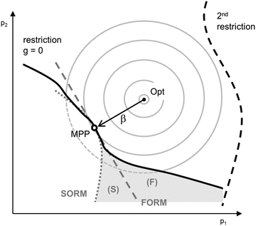

  

  Second restriction and non-conservativeness of FORM (F) and SORM (S)

• the normalization of the random variables requires a good guess of the mean and standard deviation of the multidimensional random variables which may be found only after a large number of tests;

• the approaches primarily hold only for one critical restriction, and they may fail or become less applicable as soon as there is a second restriction active as shown in Fig. 6.3.

As the proposed approaches to carrying out reliability and robustness studies consume much time and computing power, faster steps to come up with acceptable results were proposed (Gekeler and Steinbuch 2014). These proposals, found by the optimization techniques, may be used as input for manufacturing without having to consider uncertainty at all.

To take into account stochastic problems, a more general definition was suggested. The objective function is described as:

$$ \mathbf{z}=\mathbf{z}{\left({p}_1,{p}_2,\dots, {p}_{np}\right)}^T, $$

(6.5)

where z is a vector composed of two other vectors, s and r:

$$ \mathbf{z}={\left(\mathbf{s},\mathbf{r}\right)}^T={\left({s}_1,{s}_2,\dots, {s}_{n_g},{r}_1,{r}_2,\dots, {r}_m\right)}^T, $$

(6.6)

Here s stands for the vector of n _g optimization goals , while r represents the set of m restrictions . We confine the idea here to single-objective optimization i.e. $\mathbf{s}={s}_1$. In general there are given limits to the design parameters like before

$$ {p}_{i, \min}\le {p}_i\le {p}_{i, \max },i=1\dots {n}_p. $$

(6.7)

In addition all p _i may show some scatter indicated by

$$ {p}_i={p}_i\pm \varDelta {p}_i. $$

(6.8)

As mentioned above, some authors, e.g., (Wang et al. 2010), distinguish sets of non-scattering design or optimization parameters d, scattering design or optimization parameters X, and scattering non-optimization parameters C. If one allows $\varDelta {p}_i=0$ for some set of parameters and ${p}_{i, \min }={p}_{i, \max }$ for another set or even the same set of the same parameters, these three classes will be reduced to one set of optimization parameters p as proposed in Eqs. (6.5)–(6.8). Some of them do not essentially scatter , and some of them are fixed within their tolerances. This allows for a more simple annotation without losing the generality of the idea.

The main concern of stochastic mechanics is to use a sufficient amount of test data to provide acceptable probabilistic measures. One common and efficient way to solve this problem is using a Response Surface (RS , cf. Sect. 2.7) approach in all components of $\mathbf{z}={\left(\mathbf{s},\mathbf{r}\right)}^T$. It provides an approximation of the distribution and allows for an estimation of the mean and standard deviation of all the components of z. In this formulation, the goal and the restrictions are defined respectively as s and r.

In most cases, RS are often first or second order degree polynomials (cf. Sect. 2.7) in the optimization parameters. Since frequently better data are not available, one may use them to perform the reliability or the robustness analysis. The main disadvantage of this approach is that a large number of tests are required (i.e. FE-jobs or experimental measurements). The RS is defined by its coefficients:

$$ RS\left({p}_1,{p}_2,\dots, {p}_{np}\right)={a}_0+{\displaystyle \sum_i}{a}_i{p}_i+{\displaystyle \sum_i{\displaystyle \sum_{k\le i}{a}_{ik}{p}_i{p}_k}}. $$

(6.9)

The number of coefficients for a second order Response Surface is

$$ {n}_c={n}_p+1+\left({n}_p+1\right){n}_p/2, $$

where n _p denotes the number of optimization parameters. Non-design parameters C as defined at the beginning of this section might be omitted to reduce the number of studies. To find the RS by a least squares method, the number of tests should be about twice the number of coefficients. In consequence one ought to run approximately n ² _p tests. For large nonlinear studies and some (e.g., ${n}_p=10$ ) optimization parameters, where one job may take some hours, the total computation time may become absolutely unacceptable. Reduction of the number of coefficients in Eq. (6.9) by omitting the mixed terms to

$$ RS\left({p}_1,{p}_2,\dots, {p}_{np}\right)={a}_0+{\displaystyle \sum_i}{a}_i{p}_i+{\displaystyle \sum_i}{a}_{ii}{p}_{ii}^2 $$

(6.10)

may sometimes help to accelerate the process, as there are only $2{n}_p+1$ unknowns and one has to run about 4n _p tests. But this simplification may essentially reduce the quality of the approximation. The response surfaces found by any means may be used to estimate the goal or the reliability as shown in Fig. 6.4. The short vertical lines indicate the test data and their distance to the RS .

Fig. 6.4

Approximation of a goal or restriction by a second order response surface

To continue, it is assumed that the RS are sufficiently good representations of the distribution of the studies’ results. The estimation of the reliability by using the RS can be done afterwards. It would be appropriate to assume the RS to be scattering as well. Their standard deviation might be guessed from the deviation of the difference between the RS and the test data

$$ {\sigma}_{RS}^2=\frac{1}{n-1}\sum_{i=1}^n{\left( test\left({\mathbf{p}}_i\right)-RS\left({\mathbf{p}}_i\right)\right)}^2. $$

(6.11)

Here p _i represents the vector of all design variables at the test # i including the scattering and non-scattering design variables. It is evident, that the better the Response Surface is able to represent the data, the smaller the estimated standard deviation σ ² _RS becomes.

In many cases the optimum and the MPP (cf. Fig. 6.3) coincide. If the random variables are following normal distributions, one may find the probability at parameter values from the mean and the standard deviation. The reliability close to the MPP and Optimum becomes 50 % because $\beta =0$. In consequence, one has to move away from the MPP along the gradient of the restriction into allowed ($g<0$) regions. In this way the distance to not only MPP but also to the optimum will be increased to raise the reliability.

A high quality of the Response Surfaces to reproduce the data input makes the prediction of the failure probability more realistic and not over-conservative. In Fig. 6.5, the deterministic reliability curves correspond to 50 % if MPP = OPT. To improve the reliability, the corresponding scatters of the restriction and the proposed design have to be taken into account.

Fig. 6.5

Reliability and scatter , dots indicate the combined probability of goal and restriction

The assumption of a normal distribution of all random variables may cause large standard deviations. This decreases the power of the always doubtful stochastic  statements. To reduce both weak components and to improve the performance, better approximations for the distributions could be used. With knowledge of the type of the distributions and their moments, they can be used for some or all optimizations. It is assumed that the random variables , optimization parameters and the scattering design data are each distributed independently. Then the total probability density will be the product of the probability density pr _i of the parameters:

$$ P{r}_{total}={\displaystyle {\prod}_{{}_i}}p{r}_i\left({p}_i\right),i=1,\dots, {n}_p $$

(6.12)

For all of the parameters’ distributions, the quality of approximation is tested by using different known distributions such as, e.g., normal, uniform, Chi-squared, log-normal, Poisson, Maxwell, Weibull or any other distributions that are assumed to be helpful. The squared error between all configurations of the distributions is minimized with appropriate moments (μ, σ) and the test data available:

$$ min\Big( error{\left(\left(P{r}_{total}\left({p}_i\right)- test\left({p}_i\right)\right)\right)}^2 $$

(6.13)

This minimization may be done by a bionic approach to deal with local optima. This optimization helps to find estimates for the distribution’s moments that produce good approximations. Even if this search requires many loops to check all possible combinations of distributions, the time for this search will be smaller compared to the time required for real FE-jobs.

After selecting an appropriate distribution, the problem of estimating the resulting failure probability still remains. For a normal distribution, one can measure the length of the β-vector and compare its length to the standard deviation. For mixed type product distribution and scattering restrictions, a realistic guess of the length and the interpretation of β are required. This question may be solved by some tests of the design on the line between optimum and MPP or along the gradient of the restriction g through the MPP. From these tests, approximations of the distribution and the failure probability will be derived.

In many cases the optima found lie close to a restriction . In these cases, neither reliability nor robustness requirements are fulfilled. If such an optimized design does not provide sufficiently high reliability or robustness, its free parameters must be modified to shift it away from the critical regime . This may be done by translating the parameters along a direction close to the normal β or the gradient of the restriction g from the MPP in Fig. 6.1. The normal on the restriction may not be the direction of the fastest improvement of the reliability as long as the normalized normal distribution is not used. Studies, such as the ones on the response surfaces, may help to give acceptable representations of the preferable position of the design. Care should be taken in the presence of more than one restriction (Fig. 6.3). If other restrictions prohibit feasible solutions near the optimum, we need to search other regions of the parameter space which are large enough to allow for solutions that do not violate any restriction.

Example 6.1

We analyze the bending of an L-Profile fixed at its lower end while a deflection of the upper end of 400 mm is applied. The goal is the minimization of the mass of L-Profile. The length L ₁ and thickness T are defined as free parameters (Fig. 6.6).

Fig. 6.6

L-Profile under displacement controlled bending load. (a) Overall view. (b) Free parameters L ₁ and T

Figure 6.7 indicates the meaning of the constraints on the force and energy.

Fig. 6.7

Definition of constraints on force and energy

• Force $F(u)<{F}_{\max }$,

• $$ F\left({u}_{\max}\right)>{F}_{\min } $$

• ${W}_{mech}>{W}_{\min }$.

In order to generate the corresponding response surfaces, one needs to place variants in the parameter space. This can be done using, for example, the Latin Hypercube Sampling method. Afterward, response surfaces for the goal and the constraints will be generated. Then the restrictions are applied to the Response Surfaces (see Fig. 6.8).

Fig. 6.8

Response Surface with applied restrictions for L-Profile

The optimization is done on the response surface of the mass in order to find the deterministic optimum . The search for the optimum without taking into account the scattering is indicated in Fig. 6.9.

Fig. 6.9

Optimization on RS , which represents the mass in the acceptable parameter region

Now the reliability and robustness of the optimum must be guaranteed. We do it by stepping away from the limits of the allowed parameter region, following the expected scatter (Fig. 6.10). The quantification of this scatter must be provided by real-world experiences of the manufacturing process and the material quality.

Fig. 6.10

Guess reliability and robustness by the use of the expected scatter of the input data

6.1.6 Conclusion

The question of robustness and reliability in optimization problems under uncertainties must be studied with the aim of providing applicable strategies that may be used in the design process. The proposed methods may help to understand of the basic concepts.

As often only small numbers of test results or data of FE-Jobs are available, the quality of the probabilistic interpretation should be considered with care. Approximations using normal distributions include the danger of being non-conservative and, in addition, may produce large scatter predictions , thus reducing the predicted reliabilities.

Adapted approximations may reduce the scatter and yield more realistic predictions . If many restrictions must be considered, the search for regions with feasible designs may become more tempting than the original optimization. In all cases, the inherent uncertainties of such stochastic approaches need to be taken into account, especially if the safety of human beings or large costs of failures are to be considered. In every case, the rules of probability must not be disregarded to guarantee a sufficient level of theoretical reliability .

6.2 Multi-Objective Optimization

• Nico Esslinger 

In the previous chapters, we discussed mono-objective optimization. The goal there was to find the minimum or maximum of a defined scalar objective function. In some cases, it may be difficult to define a problem with just one objective function. Using just one objective function can also lead to a bias during the modeling phase.

To eliminate this limitation, the idea of Multi-Objective Optimization (MOO ) was developed. MOO handles problems with more than one objective function. For example, we take the weight and the stress of a component as simultaneous goals in the same optimization study.

6.2.1 Terms and Definitions

The introduction of multiple objective functions lead to the following mathematical problem:

$$ \mathrm{minimize}/\mathrm{maximize} \mathbf{z}\left(\mathbf{p}\right) $$

In this equation z(p) is a vector whose components contain the value of the different objective functions, p are the free parameters and g(p) stands for the constraints . We now have to define what we understand as the minimum of a vector. We avoid this undefined situation if we look not at only one unique solution of the optimization, but at a set of solutions Ω_t. The interesting solutions of Ω_t are often called Pareto solutions. A Pareto optimum is a point in Ω_t where it isn’t possible to improve one goal without decreasing another goal at the same time (Coello Coello 1999). The set of Pareto solutions after the Multi-Objective Optimization is called the tradeoff surface . In Fig. 6.11, we see an abstract set of solutions Ω_t plotted in the (z ₁, z ₂)-plane. The subplots show the tradeoff surface for the different kinds of optimization.

Fig. 6.11

Different types of Multi- Objective Optimization with two objective functions. (a) Minimize z ₁, minimize z ₂. (b) Minimize z ₁, maximize z ₂. (c) Maximize z ₁, maximize z ₂. (d) Maximize z ₁, minimize z ₂

Tradeoff surfaces can assume many different shapes. The simplest one is the convex surface shown in Fig. 6.11. But it is also possible that the Pareto -surface is not convex (Fig. 6.12a) or consists of unconnected segments (Fig. 6.12b).

Fig. 6.12

Possible shapes of the tradeoff surface when minimizing two objective functions. (a) Non-convex tradeoff surface . (b) Tradeoff surface with unconnected segments

Example 6.2

As an example, we use a hollow beam under a given load F. The optimization problem is shown in Fig. 6.13. As optimization parameters, we use the height p ₁ and the width p ₂ of the rectangle inside of the hollow beam. The outside dimensions h, w and l are constant during the optimization.

Fig. 6.13

The structure of the hollow-beam problem

The goal is to minimize the mass m, as well as to minimize the maximum displacement d of the hollow beam under the load F. The mass is calculated by

$$ {z}_1\left({p}_1,{p}_2\right)=m\left({p}_1,{p}_2\right)=\left(w\cdot h-{p}_1\cdot {p}_2\right)\cdot l\cdot \rho . $$

The maximum displacement d is calculated by

$$ \begin{array}{l}{z}_2({p}_1,{p}_2)=d({p}_1,{p}_2)=\frac{F\cdot {l}^3}{3\cdot E\cdot {I}_y({p}_1,{p}_2)},\\ {}\\ {}\mathrm{w}\mathrm{i}\mathrm{t}\mathrm{h}\text{\ }{I}_y({p}_1,{p}_2)=\frac{w\cdot {h}^3-{p}_2\cdot {p_1}^3}{12}.\end{array} $$

Our design space is restricted by the upper and lower limit of the two input parameters. The range is

$$ 10\le {p}_1,{p}_2\le 14. $$

The constant values for geometry and material are shown in Table 6.1.

Table 6.1 Input data used in the hollow-beam problem

In Fig. 6.14 we see the set of possible results for the objective functions within the parameter range. To generate this set, we randomly choose some values for the parameters with p ₁, p ₂ ϵ[10, 14] and calculate the values of the objective functions. The set of solution is plotted in the (z ₁, z ₂)-plane. In this example we can see that there is not one singular solution with a minimum weight z ₁ and a minimum displacement z ₂.

Fig. 6.14

Tradeoff surface of the hollow-beam problem

6.2.2 Strategies for MOO

In the previous example, we found the tradeoff surface by calculating many designs and extracting the tradeoff surface from the results. This method is not very efficient because we get many designs which we are not interested in. To calculate the Pareto optimal points or the tradeoff surface directly, there are many different methods available. The following list shows the most used methods to calculate the tradeoff surface.

• Compromise Method

• Weighted-Sum

• Distance-to-a-reference -objective Method

  In this method we define a reference point with values for each objective function. The new goal is to minimize the distance between the result of the objective function and the selected reference point.

• Multiple Objective Genetic Algorithm (MOGA)

  MOGA handles the multiple objective functions within the genetic algorithm. It uses the values from each individual to calculate a corresponding efficiency. The selection of the parents in the next iteration is in proportion to the efficiency.

There are many more methods to solve MOO problems. A good overview of most of them can be found in (Collette and Siarry 2004). In the following sections we will discuss the Compromise Method and the Weighted Sum in detail.

6.2.2.1 Compromise Method

The Compromise Method allows us to transform a Multi-Objective Optimization problem into a mono-objective optimization problem with additional constraints. Therefore, we choose one objective function as the remaining goal for the optimization. The k-1 additional objective functions are transformed into inequality constraints. If we choose the first objective function z ₁ as the remaining goal, the optimization problem is transformed as follows:

$$ \begin{array}{l}\mathrm{minimize} {z}_1\left(\mathbf{p}\right)\\ {} {z}_2\left(\mathbf{p}\right)\le {\varepsilon}_2\\ {} \vdots \\ {} {z}_k\left(\mathbf{p}\right)\le {\varepsilon}_k\\ {} \mathbf{g}\left(\mathbf{p}\right)\le 0\end{array} $$

For an optimization task with initially two objectives, this new formulation leads to an optimization problem visualized in Fig. 6.15. Here the second objective function z ₂ is constrained by the value ε ₂. The goal is to minimize the objective function z ₁. As result we obtain one Pareto point z _1,min .

Fig. 6.15

Behavior of the compromise method

For the identification of other Pareto points and to obtain a tradeoff surface with this method, we perform multiple optimization runs and vary the value ε ₂ of the restricted objective function z ₂.

Example 6.3

To get an idea how the tradeoff surface is calculated in a real problem, we use the hollow-beam problem introduced in Example 6.2. The objective function z ₁ is defined as the goal. The objective function z ₂ is transformed into a constraint. As we expect displacement values d in the range of 0…0.6 mm within the defined parameter range, we choose five values 0.2, 0.3, 0.4, 0.5 and 0.6 for the constraint value ε ₂. In Fig. 6.16, we see the Pareto optima for the five constraints. We realize there is one severe disadvantage of this method. Due to the shape of the tradeoff surface, there is no point calculated between the mass m = 40 and m = 80, so we have no idea about the Pareto front in this region.

Fig. 6.16

Compromise method for the hollow-beam problem

This might be resolved by switching the goal and restricting the objective z ₁ (the mass of the hollow beam) with values ε ₁ in the range of m = 40…80.

6.2.2.2 Weighted Sum

The Weighted Sum method is also a very common method to solve MOO problems (Marler and Arora 2010). Just as the Compromise Method, we try to convert the problem into a mono-objective optimization problem. Therefore, we build a resulting objective z _eq by a weighted sum of the different partial objectives  and by an appropriate set of weights w _i .

$$ {z}_{eq}\left(\mathbf{p}\right)={\displaystyle \sum_{\mathrm{i}=1}^{\mathrm{k}}}{w}_i\cdot {z}_i\left(\mathbf{p}\right) $$

(6.14)

By adjusting the weight for each objective function, it is possible to define the importance of each value for the optimum. This new formulation leads to the behavior shown in Fig. 6.17.

Fig. 6.17

Behavior of the Weighted-Sum method. (a) Convex tradeoff surface . (b) Non-convex tradeoff surface

The line L ₁ represents the relation of the weighting factors . In Fig. 6.17a, we get one unique solution, here with an equal weight for both objective functions. By variation of the weights, we get different Pareto optimal points on the tradeoff surface . In Fig. 6.17b, we can see that the basic Weighted-Sum method cannot cover non-convex areas of the tradeoff surface. This is the biggest drawback of this method so extended methods attempt to overcome this issue (Kim and de Weck 2006).

Example 6.4

As an example, again we use the hollow-beam problem (Example 6.2). The two objective functions z ₁(p ₁, p ₂), the mass, and z ₂(p ₁, p ₂), the displacement, are transformed into the new goal function

$$ {z}_{eq}\left(\mathbf{p}\right)={w}_1\cdot d\left({p}_1,{p}_2\right)+{w}_2\cdot m\left({p}_1,{p}_2\right). $$

The values of the displacement and the weight must be normalized, because they don’t share the same units. We choose five combinations [0.3, 0.7], [0.4, 0.6], [0.5, 0.5], [0.6, 0.4] and [0.7, 0.3] for the weights [w ₁, w ₂]. In Fig. 6.18 we see the resulting Pareto optima.

Fig. 6.18

Weighted Sum method for the hollow beam problem

6.3 Optimization and Process Management of the Virtual Development Process

• Rolf Steinbuch 

Among the most important but most troublesome tasks in CAE is the management of large amounts of data. Increased Quality Assurance (QA) requires the documentation of every step, every component and every detail of the virtual product development and the real lifetime of a system. This affects the design process as well. Because the optimization is included in the design, the optimization process together with all its assumptions has to be documented as well. But it is impossible to collect all the ideas designers had while working during the virtual development. A collection of all misleading ideas would only add to the overflow of stored data, which nobody is ever going to look at again.

But all this searching and trying and pursuing misleading directions creates a rich experience-based knowledge that should be available to the next subsequent projects. Design teams are supposed to produce a history of what to do, when and why. We are not discussing if this needs to be integrated in the Product-Lifecycle-Management (PLM) systems or not. But not building up a system of knowledge  leads teams to repeated errors that could be easily avoided.

An external summary of the main results to the PLM system should be done as soon as there are results found that could be generalized. In Sect. 5.1, e.g., one of the results was that, for the specific problem, Evolutionary Strategies were preferable to Particle-Swarm Optimization. This could be kept in mind and be used as a rule for this type of problem for the specific research group.

On the other hand, all the input necessary to do the robustness and reliability studies will not work without a close interaction with the component’s total data. Therefore we need to access the PLM to learn about scatter, defined and supposed uncertainties, expected misuse and critical environmental conditions. So documentation of both input and output of the optimization studies needs to become part of the process management . Unfortunately, many designers and optimization analysts are not very fond of documentation. So it remains an ongoing task to convince them that they are not merely contributing to the documentation but that they are really profiting from QA. It is worth it, and without it, there is no future for high level development.

References

Coello Coello, C. A. (1999). An updated survey of evolutionary multiobjective optimization techniques: state of the art and future trends. In Proceedings of the 1999 Congress on Evolutionary Computation, 1999, CEC 99 (Vol. 1, pp. 13). doi:10.1109/CEC.1999.781901.
Collette, Y., & Siarry, P. (2004). Multiobjective optimization: Principles and case studies. Berlin: Springer.
Du, X., & Chen, W. (2004). Sequential optimization and reliability assessment for probabilistic design. ASME Journal of Mechanical Design, 126, 225–233.
Du, X., Sudjianto, A., & Chen, W. (2004). An integrated framework for optimization under uncertainty using inverse reliability strategy. ASME Journal of Mechanical Design, 126, 562–570.
Gekeler, S., & Steinbuch, R. (2014). Remarks on robust and reliable design optimization. METAHEURISTICS AND ENGINEERING, 15th Workshop of the EURO Working Group. S. 77–82.
Kim, I. Y., & de Weck, O. L. (2006). Adaptive weighted sum method for multiobjective optimization: A new method for Pareto front generation. Structural and Multidisciplinary Optimization, 31, 105–116.
Marler, R. T., & Arora, J. S. (2010). The weighted sum method for multiobjective optimization: New insights. Structural and Multidisciplinary Optimization, 41(6), 853–862.
Tu, J., Choi, K. K., & Young, H. P. (1999). A new study on reliability-based design optimization. ASME Journal of Mechanical Design, 121, 557–564.
Wang, Z., Huang, H., Liu, Y. (2010). A unified framework for integrated optimization under uncertainty. ASME Journal of Mechanical Design, 132(5), 051008-1–051008-8.
Yin, X., & Chen, W. (2006). Enhanced sequential optimization and reliability assessment method for probabilistic optimization with varying design variance. Structure and Infrastructure Engineering, 2, 261–275.
Author information
Authors and Affiliations
Corresponding author
Editor information
Editors and Affiliations
Rights and permissions
Copyright information
© 2016 Springer-Verlag Berlin Heidelberg
About this chapter
Cite this chapter
Steinbuch, R., Kmitina, I., Esslinger, N. (2016). Current Fields of Interest. In: Steinbuch, R., Gekeler, S. (eds) Bionic Optimization in Structural Design. Springer, Berlin, Heidelberg. https://doi.org/10.1007/978-3-662-46596-7_6
Download citation
DOI: https://doi.org/10.1007/978-3-662-46596-7_6
Publisher Name: Springer, Berlin, Heidelberg
Print ISBN: 978-3-662-46595-0
Online ISBN: 978-3-662-46596-7
eBook Packages: EngineeringEngineering (R0)