Felix Klein’s Mathematical Heritage Seen Through 3D Models

Abstract

Felix Klein’s vision for enhancing the teaching and learning of mathematics follows four main ideas: the interplay between abstraction and visualisation, discovering the nature of objects with the help of small changes, functional thinking, and the characterization of geometries. These ideas were particularly emphasised in Klein’s concept of mathematical collections. Starting with hands-on examples from mathematics classrooms and from seminars in teacher education, Klein’s visions are discussed in the context of technologies for visualisations and 3D models: the interplay between abstraction and visualisation, discovering the nature of objects with the help of small changes, functional thinking, and the characterization of geometries.

1 Introduction

1.1 Klein’s Vision for Visualisations

At the age of 23, Felix Klein (1849–1925) became a professor at Erlangen. On such occasions, professors used to give a speech. Klein’s speech, which is known nowadays as the Erlangen Programme, was published with an appendix (“notes”) containing a paragraph entitled “On the value of space perception”. Even though the history of the reception of the speech and the written publication of the programme is complicated (Rowe 1983), and although its influence is contested (Hawkins 1984), this episode reveals that at an early stage of his career, Felix Klein was already interested in the teaching and learning of mathematics and in methods of visualisation:

When in the text, we designated space-perception as something incidental, we meant this with regard to the purely mathematical contents of the ideas to be formulated. Space-perception has then only the value of illustration, which is to be estimated very highly from the pedagogical standpoint, it is true. A geometric model, for instance, is from this point of view very instructive and interesting. But the question of the value of space-perception in itself is quite another matter. I regard it as an independent question. There is a true geometry which is not, like the investigations discussed in the text, intended to be merely an illustrative form of more abstract investigations. (Klein 1893, p. 244)

Klein’s point of view has undergone some changes over the years (Rowe 1985), but the idea of visualisation remains a guiding theme in Klein’s work on teaching and learning—for example, in his “Elementary mathematics from a higher standpoint”, which was published much later, it is still quite present throughout the text. Klein was keen on using cutting-edge technology to visualise modern mathematics. The collections following his concept gather plaster models, diapositives, and newly constructed machines. According to Klein, “A model—whether it be executed and looked at, or only vividly presented—is not a means for this geometry, but the thing itself” (Klein 1893, p. 42).¹ In this text, we presents implementations of some of today’s modern technologies following Klein’s main idea to offer objects of intense study.

1.2 Four Threads of Klein’s Vision for Teaching and Learning Mathematics

Klein worked out the idea to characterise geometries using group theory very early in his career, together with Sophus Lie, as formulated in his Erlangen programme. Looking back, this is certainly one of the more important aspects in Klein’s work, as it is still the way geometries are treated today, particularly non-Euclidean geometries. Hence, this is one of the four threads discussed here.

However, we start with another topic which is even more important for Klein’s vision for teaching and learning mathematics, namely the interplay between abstraction and visualisation. For Klein, visualisations play a key role in experiences, both in geometry and other areas of mathematics. He says: “Applied in particular to geometry, this means that in schools you will always have to connect teaching at first with vivid concrete intuition and then only gradually bring logic elements to the fore.” (Klein 2016b, p. 238).

Three decades after his appointment as professor, Felix Klein developed an agenda to push mathematics in schools with the help of the teaching commission inaugurated by a society of German natural scientists and physicians. In a conference in Meran in 1905, an influential syllabus was suggested for secondary education. In the appendix for the first volume of his Elementary Mathematics from a Higher Standpoint, Felix Klein writes: “The Meran curricula, in particular, are of high significance for the reform movement. They constitute already well-established norms according to which the progress of reform movements for all changes occurring in secondary education can be assessed. Their main demands are, as has already been explained in various sections, a psychologically correct method of teaching, the penetration of the entire syllabus with the concept of function, understood geometrically, and the emphasis on applications” (Klein 2016a, p. 294).

Interestingly, he links functional thinking with geometry. More generally, Klein wanted the “notion of a function according to Euler” to “penetrate (…) the entire mathematical teaching in the secondary schools” (Klein 2016a, p. 221). In particular, he very much wanted to implement calculus at school: “We desire that the concepts which are expressed by the symbols $y = f\left( x \right)$, $\frac{dy}{dx}$, $\int {y\,dx}$ be made familiar to pupils, under these designations; not, indeed, as a new abstract discipline, but as an organic part of the total instruction; and that one advance slowly, beginning with the simplest examples. Thus one might begin, with pupils of the age of fourteen and fifteen, by treating fully the functions $y = ax + b$ (a, b definite numbers) and $y = x^{2}$, drawing them on cross-section paper, and letting the concepts slope and area develop slowly. But one should hold to concrete examples” (Klein 2016a, p. 223).

A recurring topic in Klein’s teaching and research is the use of small changes to discover the nature of objects. Indeed, he started to apply this as an ongoing theme in his very early years, e.g., in his work on cubic surfaces from 1873 in which one type of surface deforms into another by a tiny change in the coefficients. In his elementary mathematics lectures, this topic is still an important method in many places, e.g., when he discusses multiple roots which transform into several nearby simple roots under small changes. Again, these studies are accompanied by visualisations to stress the related geometric aspects.

We thus identify four main ideas that describe Felix Klein’s concepts of visualisation:

• (1) interplay between abstraction and visualisation,

• (2) discovering the nature of objects with the help of small changes,

• (3) functional thinking, and

• (4) the characterization of geometries.

In the following section, these aspects are located within Klein’s work. A particular emphasis is made on 3D models, which Klein pushed strongly in his mathematical collections. Examples from recent courses at schools and universities are used to illustrate how these ideas can be approached with today’s technology.

2 Building on Klein’s Key Ideas in Today’s Classrooms and Seminars

2.1 Interplay Between Abstraction and Visualisation

2.1.1 Abstraction and Visualisation at the Core of Mathematical Activities with Geometric Objects

Imagination and abstraction have haunted philosophers for a long time, a prominent example being Kant, who—in his Critique of Pure Reason—dismissed anything empirical as being part of geometry as a scientific discipline. Hawkins (1984) points out that Klein uses “geometry” in a rather liberal way. This is somehow ironic because Klein’s Erlangen Programme significantly influenced the way mathematicians nowadays agree what geometry actually means. In this very text, he works out the role of visualisation for geometry: “Its problem is to grasp the full reality of the figures of space, and to interpret—and this is the mathematical side of the question—the relations holding for them as evident results of the axioms of space perception” (Klein 1893, p. 244).

For Klein, any object, whether “observed or only vividly imagined”, is useful for working geometrically as long as it is an object of intense study. Later, in his lectures entitled Elementary Mathematics from a Higher Standpoint, he makes clear that the main role of objects of study is to enhance the interplay between abstraction and visualisation: “One possibility could be to renounce rigorous definitions and undertake to construct a geometry only based on the evidence of empirical space intuition; in his case one should not speak of lines and points, but always only of “stains” and stripes. The other possibility is to completely leave aside space intuition since it is misleading and to operate only with the abstract relations of pure analysis. Both possibilities seem to be equally unfruitful: In any case, I myself always advocated the need to maintain a connection between the two directions, once their differences are clear in one’s mind.

A wonderful stimulus seems to lay in such a connection. This is why I have always fought in favour of clarifying abstract relations also by reference to empirical models: this is the idea that gave rise to our collection of models in Göttingen.” (Klein 2016c, p. 221).

Following this line of thought, a suitable task design involving geometric models offers both opportunities for empirical experiences and the requirement to build up abstract concepts.

2.1.2 The Interplay of Abstraction and Visualisation with 3D Printing from Grade 7

The celebrated opportunities of 3D printers surely involve a great deal of mathematics. However, while a CAD programme makes use of mathematics, it becomes invisible. Shapes can be constructed without any need for abstraction, and the software creates files that 3D printers transform to create objects. Instead of disguising mathematics in such a way, we report an approach that works at the interface of computers to 3D printers. An example of this interface is the STL-code (STereoLithography code), which describes the tessellation of a surface—namely, the boundary of a solid.

This tessellation is done in triangles; the STL-code lists the corners of these triangles. For complicated shapes, the printer needs the normal vector pointing to the exterior of the solid. Table 10.1 represents the part of the code for the triangle $\Delta f\left( {0,4,4} \right),\left( {4,4,0} \right),\left( {0,4,0} \right),$ which has the normal vector $\left( {0,1,0} \right)$.

Table 10.1 Part of an STL code for a triangle

Curved surfaces need thousands of triangles to approximate the shape in a seemingly smooth way. The code has been introduced to various groups in lower grades with the trick of limiting ourselves to polytopes. Their boundary can be triangulated in finitely many triangles very accurately, which avoids all questions of approximation. It is important, however, to have some experience with 2D coordinates. The introduction of a third coordinate did not cause severe problems in our cases.

Variants of two tasks particularly enhanced the interplay between abstraction and visualisation. They have been tried in various groups of students from grade 7 on.

First task type from abstraction to visualisation: The following task provides an STL code of a polyhedron and asks to figure out its shape. The triangulation of a cube’s surface often leads to first guesses which prove to be correct. For instance, if twelve triangles are used to triangulate the six squares, a first guess can be a dodecahedron. A rewarding discussion provides criteria as to when two triangles lie in the same plane (Emmermann et al. 2016) (Fig. 10.1).

Fig. 10.1

Photo by Halverscheid (2016)

Visualizing the triangulation of a cube by 7th graders.

Fig. 10.2

Photo by Halverscheid (2016)

Activity on tetrahedral tilings.

Second task type from visualisation to abstraction: With a number of congruent regular tetrahedra, the experimental task is to determine whether these can be used for a tessellation of space without any holes (Fig. 10.2). A cognitive conflict causes trouble because eyesight cannot decide whether there is indeed a hole or whether some of the tetrahedra’s movability is due to some artefacts in the production process of the tetrahedra. This problem can be answered by measuring activities with 7th graders or, more accurately, with the later help of the analytic geometry of angles.

In fact, determining whether packing of tetrahedra minimises the missing space is an open and hard problem.

2.2 Discovering the Nature of Objects with the Help of Small Changes

Applying small changes to a formula or an equation was one of the most natural things to do for Klein. Indeed, this was one of his main guiding themes in his early years as a mathematics researcher. As we will see, this point of view also became an important aspect of his teaching.

2.2.1 Small Changes

As a first example of Klein’s teaching of mathematics with respect to small changes, let us look at the first section on algebra in his book on elementary mathematics (Fig. 10.3). Upon opening the book to this page, one immediately notices that there is a figure. As mentioned in the previous section, Klein always tries to explain abstract mathematics with the help of drawings.

Fig. 10.3

Varying a parameter. From the first page of the first section in the algebra chapter of Klein’s book on elementary mathematics from a higher standpoint (Klein 2016a, p. 91)

However, another aspect catches the eye: the fact that he considers a function with a parameter lambda as his very first example. This clearly reflects his idea that one should always try to understand the true nature of mathematical objects. To give an example, let $y = x^{3} - x + 1$. This is a function with one variable of degree three with one real root. Yet, this example does not reflect the nature of polynomial functions of degree three in an adequate way. Only by introducing parameters such as in $y = x^{3} + px + q$ can one realise that such functions may indeed have up to three roots and that a special case seems to be that of two roots with one of them doubled. This brings Klein to the study of discriminants in order to understand whole classes of mathematical objects globally.

The crucial points of these studies of classes of mathematical objects are the moments when essential things change; in the example of cubic functions above, this is the case when—suddenly—the function no longer has one real root but two and then even three. Klein realizes that one may thus reduce much of the study of the global picture to a local study in such special cases. To give an even simpler example, take $y = x^{2}$. When looking at small changes to this function, one realises that the single root indeed splits up into two different roots. Thus, to reflect the true nature of the single root, one should count it as a double root. Of course, algebraically, this can also be seen by the fact that the factor x appears twice in the definition of the function. Today’s dynamic geometry systems now provide this as a standard technique for school teaching: a slider allows these small changes to be experienced interactively (Fig. 10.4).

Fig. 10.4

A small change reflects the true nature of the single root—which should be indeed counted twice

Klein deepens the understanding of concepts wherever appropriate. For functions in one variable, their roots are certainly one of the more important features. Thus, in the section on algebra in his elementary mathematics book, he spends quite some time on roots of functions with algebraic equations and—again—discusses this topic in a very visual and geometric way. From the well-known formula for roots of a polynomial of degree two in one variable $x$ with the equation $y = x^{2} + px + q$, it is immediate to see that it contains a single double root if and only if the so-called discriminant $p^{2} - 4q$ is zero. Thus, geometrically, all points on the parabola q = ¼p² in the pq plane yield plane curves $y = x^{2} + px + q$ with a double root; all points above this curve (i.e., where q > ¼p²) correspond to functions with no real root, and all points below correspond to functions with two real roots.

Similarly, one can study the parameters $p$ and $q$ for which the cubic polynomial $y = x^{3} + px + q$ has a double root—these are all points on the discriminant plane curve with equation $27q^{2} = - 4p^{3}$, a curve with a cusp singularity at the origin. For studying the numbers of roots of a polynomial of degree four, with $x^{4} + ax^{2} + bx + c$, one has to work with three parameters—$a,b$, and $c$—so that the parameter space is three-dimensional. In this case, all points $\left( {a,b,c} \right)$ yielding polynomial functions of degree four with a double root lie on a discriminant surface in three-space of degree 6 with a complicated equation. Because of its geometry, this discriminant surface is nowadays sometimes called a swallowtail surface. As in the case of the parabola, the position of a point $\left( {a,b,c} \right)$ with respect to the discriminant determines exactly which number and kind of roots the corresponding function of degree four possesses. Because of this feature, this discriminant surface had already been produced as a mathematical model during Klein’s time, and Klein shows a drawing of it in his elementary mathematics book. To give an example of this close geometric relation, consider our modern 3D-printed version, which even shows the non-surface part of this object—half of a parabola (see Figs. 10.5 and 10.6) . Points $\left( {a,b,c} \right)$ on this space curve correspond to functions $x^{4} + ax^{2} + bx + c$ with two complex conjugate double roots. Klein was fascinated by these connections; he discussed such aspects frequently in both his research and his teaching. For example, in his introductory article to Dyck’s catalogue from 1892 for a famous exhibition of mathematical and physical models (Dyck 1892), Klein discusses how discriminant objects describe in detail how small changes to coefficients of a function change its geometry.

Fig. 10.5

The discriminant surface of a polynomial function of degree four (Klein 2016a, p. 105)

Fig. 10.6

A 3D-printed mathematical sculpture by the second author showing this object

Klein applies exactly the same ideas to many other cases. To discuss just the simplest spatial one here, take the double cone consisting of all points $\left( {x,y,z} \right)$ satisfying the equation $x^{2} + y^{2} = z^{2}$. Similar to the case of the parabola where the sign of epsilon in y  =  x² ± ε decides about the geometry around the origin, the same happens with $x^{2} + y^{2} = z^{2} \pm \varepsilon$. Indeed, the two conical parts of the double cone meet in a single point, but for $\varepsilon > 0$, the resulting hyperboloid consists of a single piece, whereas for $\varepsilon < 0$, the resulting hyperboloid is separated into two pieces.

In 1872, Klein already had the idea that such local small changes could be used to understand the global structure of large families. Indeed, when Klein presented his model of the Cayley/Klein cubic surface with four singularities during the meeting at Göttingen in 1872 where Clebsch presented his diagonal surface model, he thought that it should be possible to reach all essential different shapes of cubic surfaces [as classified by Schläfli 1863, see (Labs 2017)] by applying different kinds of small changes near each of the four singularities independently, as published by Klein in 1873. For example, when deforming all four singularities in such a way that they join the adjacent parts (thus looking locally like a hyperboloid of one sheet), one obtains a smooth cubic surface with 27 real straight lines—one of the most classical kinds of mathematical models (Fig. 10.7).

Fig. 10.7

Photos from Klein (2016c)

The Cayley/Klein cubic surface with four singularities (left image) was Klein’s starting point to reach all kinds of cubic surfaces with the help of small changes in 1872/73, such as a smooth one with 27 straight lines (right image, Clebsch’s diagonal cubic).

As a final remark to this section, note that this idea to deform a curve or a surface locally without increasing its degree does not continue to work for surfaces of higher degrees, because starting from degree 8, it is not always possible to deform each singular point independently. For example, from the existence of a surface of degree 8 with 168 singular points [as constructed by S. Endraß (Labs 2005)], it does not follow that a surface of degree 8 with 167 singularities exists, as D. van Straten computed using computer algebra.

2.2.2 3D Scanner and Singularities of Surfaces in a Mathematics Seminar for Pre-service Teachers

In a meeting report of the Royal Academy of Sciences of Göttingen of August 3, 1872, it was stated: “Mr. Clebsch presented two models, […] which refer to a special class of surfaces of the third order. […] One of the two models represented the 27 lines of this surface, the other the surface itself, a plaster model on which the 27 lines were drawn.” This surface is an example of a so-called cubic surface, defined by all points $\left( {x,y,z} \right)$ satisfying a polynomial equation of degree three (see Figs. 10.7 and 10.8, top left model).

Fig. 10.8

Photo by Halverscheid (2015)

Historical collection of models of surfaces of the third degree (cubic surfaces).

One main feature of these cubic surfaces is that they are smooth if and only if they contain exactly 27 lines. Singularities appear if the surfaces are varied and the lines become identical. One idea for a current mathematics seminar was to study the small changes in the singularities. Each participant was given one of the singular models with the following task:

• 1. Produce a 3D scan of one of the models, which results in about 70,000 points describing the area in space.

• 2. Determine an approximate third-order equation describing the scanned area.

• 3. Reprint the surface and some variations.

• 4. Compare them with the original model (Figs. 10.9 and 10.10).

  Fig. 10.9

  

  Photo by Halverscheid (2015)

  3D scan of one of the surfaces (step 1).

  Fig. 10.10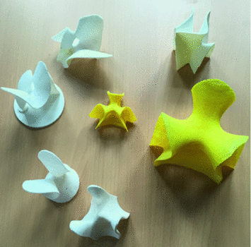

  

  Photo by Halverscheid (2015)

  3D printout of reproductions and variations of third-order surfaces (step 3).

Comparing the reproductions with the original reveals the compromises made by the producers of the original models. These compromises arise because of the accurate visualisation of surfaces as a whole and of the “singularities”. The differences also show some particular difficulties of modeling exact formulae. The reproduction and the original can often be clearly distinguished in the vicinity of singularities.

The approach taken in these seminars mainly follows the intention to use mathematical models in mathematics education (Bartholdi et al. 2016). There are, of course, more refined techniques to create such models with singularities more accurately (see www.Math-Sculpture.com by the second author).

2.3 Linking Functional Thinking with Geometry

As mentioned earlier, Klein stresses the link between functional thinking and geometry. The Meran syllabi defined “education for functional thinking” as an aim, and after World War I, functions indeed became much more prominent in secondary education in Germany. Krüger (2000) describes how “functional thinking” developed historically and how Klein used this term to strengthen mathematics in secondary education. Here, we will briefly mention some aspects appearing frequently in his elementary mathematics book which make clear that Klein had quite a broad understanding of the term “functional thinking”.

2.3.1 General Functions in Klein’s Elementary Mathematics Book

The first two examples in our section on small changes—the implicitly defined curve in Fig. 10.3 and the parabola with parameters in Fig. 10.4—are instances of Klein’s view of functional thinking. As always, Klein stresses the fact that one should visualise a function—e.g., the parabola mentioned above—as a graph to obtain a geometric picture together with the abstract formulas. However, he proceeds much further by considering not only functions from R to R but also plane curves in polar coordinates, families of plane curves, and functions in two variables.

During Klein’s time, many universities—including at Göttingen, of course—had a collection of three-dimensional mathematical sculptures illustrating important non-trivial examples for teaching purposes. One of the premier examples of those were certainly the so-called hyperbolic paraboloids, e.g., the figure given by the equation $z = xy$. From this equation, one immediately realises that the surface contains two families of straight lines, namely those for fixed values $x = a$ with equations $z = ay$ and those for fixed values of $y = b$ with equations $z = xb$. Other models show different cuts of the surface, e.g., horizontal cuts yielding a family of hyperbolas. See Figs. 10.11 and 10.12 for two historical plaster sculptures from the collection of the Mathematics Department at the University of Göttingen.

Fig. 10.11

Retrieved from http://modellsammlung.uni-goettingen.de/ on 30 May 2017, Georg-August-University Göttingen

A hyperbolic paraboloid with its two families of straight lines.

Fig. 10.12

Retrieved from http://modellsammlung.uni-goettingen.de/ on 30 May 2017, Georg-August-University Göttingen

A hyperbolic paraboloid with horizontal plane cuts.

Notice that the example of the hyperbolic paraboloid is particularly simple. In fact, in his elementary mathematics book, Klein also discusses more pathological cases such as the one given by $z = \frac{2xy}{{x^{2} + y^{2} }}$. The function is continuous everywhere, except at the origin $\left( {x,y} \right) = \left( {0,0} \right)$, where it is not even defined. Klein discusses the question of whether the function may be defined at this position in such a way that it becomes continuous everywhere. He accompanies his analytic explanations with an illustration (Fig. 10.13), which clearly shows that no unique z-value can be given for the origin because all points of the vertical z-axis need to be included into the surface to make it continuous.

Fig. 10.13

An image from Klein’s book illustrating the impossibility of extending some rational function to a continuous one. Klein copied this image from B. St. Ball’s book on the theory of screws from 1900

This example illustrates how, in his teaching, Klein tried to explain important aspects both analytically and visually to provide some geometric intuition for the mathematical phenomenon being discussed. He was not afraid of discussing pathological cases and thus often used more involved and more difficult examples in his university teaching to deepen the understanding of certain concepts, such as the example of continuous functions in the case above. Moreover, from the examples above, we see that for Klein, a function is not just a map from R to R; rather, it should be seen in a much more general way. Such examples appear frequently in his elementary mathematics book, which shows Klein’s belief that these ideas are very important for future school teachers and thus form an essential part of mathematical education.

2.3.2 General Functions in Today’s Teaching

Providing a general concept of functions is easier in today’s teaching than it was in Klein’s time due to computer visualisations. However, as with around 1900, using hands-on models—built by the students themselves, if possible—is an even better approach in some cases. Here, we want to briefly mention three examples from a seminar for teacher students, for which each session was prepared by one of the students based on at least one mathematical model. The photos in Figs. 10.14, 10.15 and 10.16 shows an interactive hyperbolic paraboloid model constructed from sheets of paper, similarly to 19th century models; an interactive ellipse drawer; and a model illustrating the definition of Bezier curves.

Fig. 10.14

Photo by Labs (2011)

A hyperbolic paraboloid, constructed by students using sheets of paper.

Fig. 10.15

Photo by Labs (2011)

Drawing an ellipse in the seminar room.

Fig. 10.16

Photo by Labs (2011)

Students work on understanding the stepwise process of creating Bezier curves.

For teaching a more general concept of functions, Bezier curves are a particularly illustrative example: First, these are functions from the interval $\left[ 0 \right.;\left. 1 \right]$ to ${\mathbb{R}}^{2}$; thus, the image is not a value but a point. Second, each of the points in the image is defined by an iterative construction process. In mathematics, students are used to defining functions by certain formulas. This can also be done in the case of Bezier curves, but in computer-aided design software, internally, it is in fact usually better to use the simple iterative process instead of quite complicated formulas.

2.4 The Characterization of Geometries

The history of an abstract foundation of geometry based just a few axioms goes back to antiquity. Yet, it took over 2000 years for the mathematical community to understand many of the essential problems involved, such as whether the Euclidean parallel axiom may be obtained as a consequence of the other axioms or not. This resulted in a new notion of “geometries” in the 19th century, particularly in different kinds of non-Euclidean geometries.

2.4.1 The Characterization of Geometries

In modern terms, the first Euclidean axioms state that for any two different points, there is a unique, infinite straight line joining them, and that for any two points, there is a circle around one and through the other. The famous antique parallel axiom essentially asserts—in modern terms—that for any straight line and any point, there is a unique line parallel to the given line through the given point. Here, parallel means that the two lines have no point in common. In the Euclidean plane, this fact seemed to be unquestionable. Yet, why should this be restricted to the Euclidean plane and to straight lines that look straight? It is possible to find abstract mathematical objects—and even geometric objects in real three-space—that satisfy all Euclidean axioms except the parallel axiom. A quite simple one may be obtained by taking the great circles on a unit sphere as “lines” and pairs of opposite points as “points”. Then, for example, for any two “points” (in fact, a pair of opposite points on the sphere), there is a unique “line” (i.e., a great circle) through those two “points” (lying in the plane through the points and the origin). For the converse, there is a difference from ordinary Euclidean geometry: any two “lines” intersect in a unique “point” (because any two great circles meet at an opposite pair of points), so there are no non-intersecting “lines”, which means that there are no parallel lines. To obtain this kind of geometry in an abstract way, one may simply replace the parallel axiom by a new one asking that for any “line” and any “point”, there is nothing parallel to the “line” through the “point”. The geometry obtained in this way is nowadays called projective geometry. Similarly, one obtains a valid geometry by asking that each line has at least two parallels.

Together with Sophus Lie—with whom Klein spent some time in Paris for research in 1870—Klein developed the idea of characterising geometries via the set of transformations leaving certain properties invariant. These transformations form the group of the geometry at hand. For example, for the familiar Euclidean plane, these are the translations, rotations, reflections, and compositions of those maps. All of them leave lengths and angles—and thus all shapes—invariant. If one allows more transformations, such as scalings in the plane, then one obtains a new geometry. As scalings are part of this group, the geometry obtained is the so-called affine plane, where lengths and angles may change but parallel lines stay parallel. A projective transformation is even more general: one just forces that lines map to lines so that parallelism is not necessarily preserved by such a transformation. The geometry obtained in this way is the projective geometry mentioned above.

The groups of transformations mentioned so far contain infinitely many elements. However, these groups have interesting finite sub-groups. Nowadays, well-known examples include all transformations leaving certain geometric objects invariant. For example, a regular $n$-gon in the plane is left invariant by $n$ rotations about its center and $n$ reflections (Fig. 10.17). In space, a regular tetrahedron is left invariant by 24 transformations. To understand and describe all of these geometrically is an interesting exercise.

Fig. 10.17

The symmetries of regular polygons, rotations and reflections: the case of the pentagon

In the 19th century, mathematicians increasingly realised that groups appear over and over again. For example, the examples with large symmetry groups were of particular interest for geometric objects defined by equations such as Kummer’s famous quartic surfaces with 16 singularities. This is one of the reasons why K. Rohn produced the tetrahedral symmetric case as a plaster model in 1877; the modern object by the second author is a smoothed version of it (see Fig. 10.18).

Fig. 10.18

A smoothed version of a Kummer surface, created by the second author (photo retrieved from http://www.math-sculpture.com/ on 5 June, 2017). Each of the 16 singularities has been deformed into a tunnel by a global small change of coefficients

2.4.2 A Spiral Curriculum on the Geometry of Tilings in a Mathematics Education Seminar

Our seminar concept meets the curricular challenge of using exhibits from past epochs for current curricula: pre-service teachers receive the subject-matter task of planning to one or only models from the third to the twelfth grade and to lead groups of different age levels. This is based on the idea of a spiral organisation of the curriculum; as Jerome Bruner put it, “any subject can be taught to act in some intellectually honest form to any child at any stage of development” (Bruner 1960, p. 33). It would now be a misunderstanding to conclude that the same lessons could be made for all grades. Rather, the intellectually honest form is concerned with the gradual transformation and adaptation of mathematical phenomena at different stages of abstraction.

For this seminar, both objects from the collection of mathematical models and instruments as well as exhibits from the wandering mathematics exhibition “Mathematics for touching” of the mathematics museum “Mathematicum” at Giessen were taken as a basis. All pre-service teachers in the seminar were given an object or group of objects along with the task of developing a theme and workshops for grades 3 through 12, and finally presenting them to small groups of 6 to 15 participants from primary through high school. During the practice, 27 pre-service teachers offered 58 workshops to a total of about 650 participants from schools.

The collection of mathematical models and instruments in the Mathematics Institute at Göttingen University is composed of models and machines, some of which are more than 200 years old. Felix Klein, who became responsible for the collection in about 1892, promoted elements of visualisation for teaching mathematics and had a vision to share mathematics with the wider public (Fig. 10.19).

Fig. 10.19

Retrieved from http://modellsammlung.uni-goettingen.de/ on 30 May 2017, Georg-August-University Göttingen

Model 331, collection of mathematical models and instruments.

In the collection are models of tessellations of the three-dimensional Euclidean space. The classification of planar and spatial lattices was intensively investigated in the nineteenth century. In 1835, Hessel worked out the 32 three-dimensional point groups; the works of Frankenheim in 1935 and Rodrigues in 1840 led to the classification of the 14 types of spatial lattices by Bravais in 1851. In 1891, Schoenflies—who wrote his habilitation at Göttingen University in 1884—and Fjedorow described these with the help of group theory. The eighteenth of Hilbert’s problems asks whether these results can be generalised: “Is there in $n$-dimensional Euclidean space also only a finite number of essentially different kinds of groups of motions with a fundamental region?” Bieberbach solved his problem in arbitrary dimensions in 1910.

Schoenflies, who wrote an instructional book on crystallography in 1923, probably designed the models for the tessellations of the Euclidean space himself. One can obtain several reproductions of two of them with the help of 3D printing and can perform this puzzle for tessellations of the Euclidean space. These reproductions were made by the KLEIN-project, whose aim is to reproduce, vary, and use models of the collection for today’s mathematics courses at schools and universities.

In relation to the level of abstraction, these questions are addressed already in the primary school. In the three-dimensional case, one can approach the questioning using the first examples—see the task from visualisation to abstraction above, which immediately illuminates that cubes have the property of filling the space, and cuboids also function in this way. The use of parallelepipeds requires more careful consideration. Schoenflies’s complete solution of the problem characterises the geometry of grids and is still used today for the systematic description of solids in chemistry and physics. The pre-service teachers arranged different activities on two- to three-dimensional tessellations (Figs. 10.20 and 10.21).

Fig. 10.20

Photo by Halverscheid (2015)

Participating high school students produce tetrahedra.

Fig. 10.21

Photo by Halverscheid (2015)

3D printouts of Schoenflies’s models as duplicates, which enable students to carry out tilings.

3 Klein’s Ideas on Visualisation and Today’s Resources for the Mathematics Classroom as an Introduction to Research Activities

As the previous section showed, visualisation is prominent within many places in Klein’s work and teaching. Content-wise, the four threads discussed are some of the major aspects involved. Regarding actual methods of teaching and learning, however, Klein pleads for activating students by letting them experience some kind of research, based on concrete examples. Indeed, at the beginning of the 1920s, Klein wrote about the beginnings of the collection of models around 1800: “As today, the purpose of the model was not to compensate for the weakness of the view, but to develop a vivid clear perception. This aim was best achieved by those who created models themselves” (Klein 1978, p. 78). Klein seems to express doubts here that the use of models in mathematics will automatically be successful. However, the use of manipulatives was characteristic for an epoche in pedagogy, which had an impact on teaching in primary schools instead of in secondary schools (Herbst et al. 2017).

He considered the deep process of creating a mathematical model as a part of teaching-learning processes to be particularly promising. In the quotation from Klein on the “weakness of intuition”, one may see skepticism glittering with mere illustrative means consumed in a merely passive way. A mere consideration of the collection of objects, in this respect, would not be without problems and would have to be accompanied by activating formats. In the task orientation of the scientific and mathematical studies, the usage of historic models, computer-aided presentations, and 3D-printed models can be an opportunity for providing tasks with a product-oriented component.

In this way, Klein’s quotes show him as a constructivist, with a striking feature of his work being the idea of enabling students to carry out suitable mathematical operations (Wittmann 1981). At the same time, he considers the “genetic method” an important argument for the confrontation with or the construction of models because they allow an approach to mathematics using several methods: “In particular, applied to the geometry, this means: at school, one would have to provide a link to the vivid, hands-on visualisation and can just slowly move logical elements to the foreground”. He continues: “The genetic method alone will prove to be justified to allow the student slowly to grow up into these things”. As research objects, models address all levels of expertise. Klein seems to warn people not to underestimate methods to approach mathematics in different levels, when he asks, “Is it not just as worthy a task of mathematics to correctly draw as to correctly calculate?” (Klein 1895, p. 540). For him, tools for visualisation are an ongoing mathematical activity at all levels. The selection of the four major threads presented in this article illustrates this via examples from both Klein’s own research and his teaching.

References

Bartholdi, L., Groth, T., Halverscheid, S., & Samuel, L. (2016). Mathematische Modelle zur Entwicklung und Vernetzung von Modulen in der Lehrerbildung. In C. Weber, et al. (Eds.), Objekte wissenschaftlicher Sammlungen in der universitären Lehre (pp. 63–70). Berlin: Humboldt-Universität zu Berlin. https://edoc.hu-berlin.de/handle/18452/2078, https://doi.org/10.18452/1426.
Bruner, J. S. (1960). The process of education. Cambridge: Harvard University Press.
Emmermann, L., Groth, T., & Halverscheid, S. (2016). Polytope mit dem 3-D-Drucker herstellen. Räumliches Denken und Operieren mit Koordinaten ab Klasse 7. In PM: Praxis der Mathematik in der Schule (Vol. 58, pp. 31–45). ISSN 1617-6960, 0032-7042.
Hawkins, T. (1984). The erlanger programm of Felix Klein: Reflections on its place in the history of mathematics. Historia Mathematica, 11(4), 442–470. https://doi.org/10.1016/0315-0860(84)90028-4.
Herbst, P., Fujita, T., Halverscheid, S., & Weiss, P. (2017). The learning and teaching of geometry in secondary schools: A modeling perspective. New York: Routledge. ISBN 9780415856911. https://doi.org/10.4324/9781315267593.
Klein, F. (1978). Vorlesungen über die Entwicklung der Mathematik im 19. Jahrhundert. Berlin, Heidelberg, New York: Springer.
Klein, F. (1893). A comparative view of recent researches in geometry (Dr. M. W. Haskell, Trans.). Bulletin of the New York Mathematical Society, 2(10), 215–249. https://doi.org/10.1090/s0002-9904-1893-00147-x. Available at http://www.ams.org/journals/bull/1893-02-10/.
Klein, F. (1895). Über die Beziehungen der neueren Mathematik zu den Anwendungen. Antrittsrede Universität Leipzig am 25.10.1880. Zeitschrift für den Mathematisch-naturwissenschaftlichen Unterricht, 26, 540.
Klein, F. (2016a). Elementary mathematics from a higher standpoint: Vol. I. Arithmetic, algebra, analysis. Berlin: Springer. https://doi.org/10.1007/978-3-662-49442-4.
Klein, F. (2016b). Elementary mathematics from a higher standpoint: Vol. II. Geometry. Berlin: Springer. https://doi.org/10.1007/978-3-662-49445-5.
Klein, F. (2016c). Elementary mathematics from a higher standpoint: Vol. III. Precision mathematics and approximation mathematics. Berlin: Springer. https://doi.org/10.1007/978-3-662-49439-4.
Krüger, K. (2000). Erziehung zum funktionalen Denken Zur Begriffsgeschichte eines didaktischen Prinzips. Journal für Mathematik-Didaktik, 21(3–4), 326–327.
Labs, O. (2005). Hypersurfaces with many singularities. Doctoral dissertation, University of Mainz, Mainz.
Labs, O. (2017). Straight lines on models of curved surfaces. Mathematical Intelligencer, 39(2), 15–26. https://doi.org/10.1007/s00283-017-9709-y.
Rowe, D. E. (1983). A forgotten chapter in the history of Felix Klein’s: Erlanger programm. Historia Mathematica, 10(4), 448–454.
Rowe, D. E. (1985). Felix Klein’s “Erlanger Antrittsrede”: A transcription with English translation and commentary. Historia Mathematica, 12(2), 123–141.
von Dyck, W. (1892). Katalog mathematischer und mathematisch-physikalischer Modelle, Apparate und Instrumente. München: Hof- und Universitätsdruckerei von Dr. C. Wolf und Sohn.
Wittmann, E. (1981). Beziehungen zwischen operativen “Programmen” in Mathematik. Psychologie und Mathematikdidaktik. Journal für Mathematik-Didaktik, 2(1), 83–95.
Author information
Authors and Affiliations
Corresponding author
Editor information
Editors and Affiliations
Rights and permissions
Open Access This chapter is licensed under the terms of the Creative Commons Attribution 4.0 International License (http://creativecommons.org/licenses/by/4.0/), which permits use, sharing, adaptation, distribution and reproduction in any medium or format, as long as you give appropriate credit to the original author(s) and the source, provide a link to the Creative Commons license and indicate if changes were made.
The images or other third party material in this chapter are included in the chapter's Creative Commons license, unless indicated otherwise in a credit line to the material. If material is not included in the chapter's Creative Commons license and your intended use is not permitted by statutory regulation or exceeds the permitted use, you will need to obtain permission directly from the copyright holder.
Copyright information
© 2019 The Author(s)
About this chapter
Cite this chapter
Halverscheid, S., Labs, O. (2019). Felix Klein’s Mathematical Heritage Seen Through 3D Models. In: Weigand, HG., McCallum, W., Menghini, M., Neubrand, M., Schubring, G. (eds) The Legacy of Felix Klein. ICME-13 Monographs. Springer, Cham. https://doi.org/10.1007/978-3-319-99386-7_10
Download citation
DOI: https://doi.org/10.1007/978-3-319-99386-7_10
Published:
Publisher Name: Springer, Cham
Print ISBN: 978-3-319-99385-0
Online ISBN: 978-3-319-99386-7
eBook Packages: EducationEducation (R0)