The Role of Nuclear Techniques in Biosaline Agriculture

Abstract

The major constraints under Saline Agriculture are the availability of essential nutrients and water to the plant which are adversely affected by excessive salts in the soil solution. Among the essential plant nutrients, N plays a key role in plant growth and productivity. Nuclear and isotopic techniques (also called nuclear-based techniques) are a complement to, not a substitute for, non-nuclear conventional techniques. Nuclear-based techniques, however, do have several advantages over conventional techniques by providing unique, precise and quantitative data on soil nutrient and soil moisture pools and fluxes in the soil-plant-water and atmosphere systems. Isotopic techniques provide useful information in assessing soil-water-nutrient management which can be tailored to specific agroecosystems for managing soil salinity. For example, ¹⁵N stable isotopic techniques can be used to measure rates of the various N transformation processes in soil-plant-water and atmosphere systems, such as N mineralization-immobilization, nitrification, biological N₂ fixation, N use efficiency, and microbial sources of production of nitrous oxide (N₂O), a greenhouse and ozone depleting gas, in soil. The use of oxygen-18, hydrogen-2 (deuterium) and other isotopes is an integral part of agricultural water management, allowing the identification of water sources and the tracking of water movement and pathways within agricultural landscapes as influenced by different irrigation technologies, cropping systems and farming practices. It also helps in the understanding of plant water use, quantifying crop transpiration and soil evaporation and allows us to devise strategies to improve crop production, reduce unproductive water losses and prevent land and water degradation.

1 Introduction

Among the numerous abiotic and biotic stresses that affect plant productivity worldwide, soil water stress (drought) is the most common growth limiting factor in arid and semi-arid regions (Saranga et al. 2001), followed closely by salt stress (Pessarakli 1991). Development of a sustainable agriculture will require the combined use of soil, nutrient, and water management strategies that enhance crop productivity, while at the same time reducing abiotic and biotic stresses. To reach a truly sustainable agriculture, new ‘climate smart’ agricultural practices will need to be developed and adopted by the end users. These climate smart practices include both management strategies and specific technologies, ones which enhance crop productivity, environmental sustainability and wise use (conservation) of agro-ecosystems.

The Soil and Water Management & Crop Nutrition (SWMCN) subprogram of the Joint Food and Agriculture Organization (FAO) and International Atomic Energy Agency (IAEA)’s Division of Nuclear Applications in Food and Agriculture, has developed a wide range of nuclear and isotopic techniques to enhance nutrient and water use efficiencies, increase biological N fixation through the capture of atmospheric di-nitrogen (N₂) and carbon (C) storage in salt affected soil.

2 Background Information on Isotopes

The number of protons plus neutrons present in the nucleus of an atom is called the atomic weight, while the number of protons (or electrons – which is always equal) is known as atomic number. Isotopes are defined as atoms of the same atomic number but differing atomic weight. For example, nitrogen (N) has one isotope (¹⁵N), which has the same number of protons (7) as ¹⁴N, but one extra neutron. This gives it (¹⁵N) a different atomic weight (7 + 8 = 15).

Isotopes may exist in both stable and unstable (radioactive) forms, depending on the stability of the nucleus in an atom. For example, the sulfur (S) consists of 5 isotopes (³²S, ³³S, ³⁴S, ³⁵S and ³⁶S); one of which (³⁵S) is a radioactive beta emitter, while the other four (³²S, ³³S, ³⁴S and ³⁶S) are stable. Thus, a radioactive isotope is an atom with an unstable nucleus which spontaneously emits radiation (alpha or beta particles and/or gamma electromagnetic rays). The non-stability occurs because the ratio of neutrons to protons in a nucleus lies outside the belt of stability (i.e., outside a particular number due to an excess of either protons or neutrons), which varies with each atom. In contrast, a stable isotope is an atom with a stable nucleus (i.e., the ratio of neutrons to protons in the nucleus of an atom is within the belt of stability), and hence, it does not spontaneously emit any radiation (Nguyen et al. 2011). Stable isotopes exist in light and heavy forms with heavy isotopes having a higher atomic weight than light isotopes (Table 6.1).

Table 6.1 Average abundances of stable isotopes (% abundance in brackets) of some of the major elements commonly occurring in agro-ecosystems

The quantity of a stable isotope is measured by an Elemental Analyser coupled to an Isotope Ratio Mass Spectrometer (IRMS). Thus, a sample of soil or biological material is combusted into a gas, which is fed into a mass spectrometer, where the ratio of the stable isotopes of interest (e.g., ¹³C/¹²C, ²H/¹H, ¹⁵N/¹⁴N, ¹⁸O/¹⁶O,³³S/³²S) is determined.

Radioactive isotopes (radioisotopes) are measured by their rate of ‘decay’, e.g. liquid scintillation counters are used for beta particle emitting radioactive isotopes, gamma spectrometers for gamma ray emitting radioactive isotopes and alpha spectrometers for alpha particle emitting radioactive isotopes. The international unit (SI) of activity decay is the Becquerel (Bq), which is equal to one disintegration per second (dps). The old unit commonly used was called the Curie, which is equivalent to 3.7 × 10¹⁰ dps or 3.7 × 10¹⁰ Bq (Nguyen et al. 2011).

3 Use of Nuclear and Isotopic Techniques in Biosaline Agriculture

Nuclear and isotopic techniques (also called nuclear-based techniques) are a complement to, not a substitute for, non-nuclear conventional techniques. Nuclear-based techniques, however, do have several advantages over conventional techniques by providing unique, precise and quantitative data on soil nutrient and soil moisture pools and fluxes in the soil-plant-water and atmosphere systems. Isotopic techniques provide useful information in assessing soil-water-nutrient management which can be tailored to specific agro-ecosystems for managing soil salinity. For example, ¹⁵N stable isotopic techniques can be used to measure rates of the various N transformation processes in soil-plant-water and atmosphere systems, such as N mineralization-immobilization, nitrification, biological N₂ fixation, N use efficiency, and microbial sources of production of nitrous oxide (N₂O), a greenhouse and ozone depleting gas, in soil. Several nuclear and isotopic techniques are being employed in soil water management studies. The soil moisture neutron probe is ideal in field-scale rooting zone measurement of soil water, providing accurate data on the availability of water for determining crop water use and water use efficiency and for establishing optimal irrigation scheduling under different cropping systems especially under saline conditions.

The use of oxygen-18, hydrogen-2 (deuterium) and other isotopes is an integral part of agricultural water management, allowing the identification of water sources and the tracking of water movement and pathways within agricultural landscapes as influenced by different irrigation technologies, cropping systems and farming practices. It also helps in the understanding of plant water use, quantifying crop transpiration and soil evaporation and allows us to devise strategies to improve crop production, reduce unproductive water losses and prevent land and water degradation.

For details on the principles and applications of the various nuclear and isotopic techniques in soil, water and plant nutrient studies in agro-ecosystems, the readers are referred to the IAEA Training Manuals (IAEA 1990, 2001) and the review paper published by Nguyen et al. (2011). In below section, a stepwise protocol has been described to set up a field study to quantify fertilizer use efficiency of the added fertilizer.

4 The Use of Nitrogen-15 (¹⁵N) to Study Fertilizer Use Efficiency

The major constraints under Saline Agriculture are the availability of essential nutrients and water to the plant which are adversely affected by excessive salts in the soil solution. Among the essential plant nutrients, N plays a key role in plant growth and productivity. To take up N from the soil solution, plants compete with a range of N removal processes/losses including immobilization, leaching, and gaseous emissions of N as ammonia (NH₃), nitrous oxide (N₂O), nitric oxide (NO) and molecular nitrogen (N₂) into the atmosphere. Because of these N losses, the N use efficiency (kg of dry matter produced per kg of N applied) or useful use of N by plant is invariably less than 50% of the applied N (Zaman et al. 2013a, b, 2014). The extent to which N is removed from soils, or made unavailable to plants by the above biogeochemical processes is of both economic and environmental importance.

Under saline conditions, the presence of excessive salts (especially Na⁺) in the soil solution, coupled with a high soil pH, is likely to further increase the competition between N uptake by the plant and the soil N losses, thereby reducing crop productivity further. Quantifying N use efficiency and the sources of N losses enables researchers to develop ‘technology packages’ which can enhance N uptake and minimize N losses, thus allowing for sustainable crop productivity under saline conditions.

4.1 Setting Up Experimental Field Plots

In order to determine the N fertilizer use efficiency (NUE) of a wheat crop with a high degree of accuracy, a researcher shall set up a field trial on a relatively flat site with uniform fertility and slope so as to minimize background variations of soil nutrient levels, especially N and nutrients losses via surface runoff (Fig. 6.1).

Fig. 6.1

A wheat trial set up on a flat soil

Considering an experimental trial of N fertilizer applied at four rates: zero or control (T1), low (T2), middle (T3), and high (T4) of kg N per ha, with four individual replicate plots (each plot being 7 m × 7 m) for each of the four rates of N. (see schematic diagram below – Fig. 6.2).

Fig. 6.2

A schematic diagram of experimental layout

A ‘buffer zone’ of 2 m wide on each of the four sides of the experimental site, with a 2 m wide strip between each of the individual replicate plots is especially important to prevent contamination of adjacent plots by N via surface runoff after heavy irrigation or rainfall, as well as lateral movement of N within the soil. The individual (replicate) field plots can be a range of sizes, depending on available land area, experimental design, farm resources (machinery) and most importantly available budget. Generally, a larger size for each individual replicate plot (e.g., 7 m long × 7 m wide) is considered as the best for minimizing edge effects (nutrient losses from the fertilized area to an un-fertilized area) on final crop yield, with each of four replicate plots being placed within four different treatment blocks.

• Prior to treatment application, four composite soil samples (each composite soil sample consist of ten soil cores from each experimental block) from 0–15 cm depth, shall be collected to analyze for key soil properties including, soil pH, ECe, Na⁺, Ca²⁺, Mg²⁺, K⁺, total N, total C, and Olsen P.

• First apply any soil amendments such as gypsum, and other chemical fertilizers without N (P and K as recommended) and animal manure.

• Assuming 7 m × 7 m (49 m²) replicated field plot receiving N-fertilizer in the form of granular urea (46%N) at rate of 80 kg N ha⁻¹ in two split applications during wheat growth period, the amount of urea is calculated below:

  $$ {\displaystyle \begin{array}{ll}& \mathrm{Rate}\ \mathrm{of}\ \mathrm{fertilizer}\ \mathrm{application}\ \left(\mathrm{kg}\ \mathrm{per}\ \mathrm{ha}\right)\\ {}& =\frac{100\times \mathrm{nutrient}\ \mathrm{element}\ \mathrm{required}\ \left(\mathrm{kg}\ \mathrm{per}\ \mathrm{ha}\right)}{\%\mathrm{nutrient}\ \mathrm{element}\ \mathrm{concentration}\ \mathrm{in}\ \mathrm{a}\ \mathrm{fertilizer}.}\end{array}} $$

Example:

The amount of urea for the first application (40 kg N ha⁻¹) can be calculated as.

$$\mathrm{kg}\text{of urea required}\mathrm{per}\mathrm{ha}\text{for the first application}=\frac{100\times 40}{46}=86.95\mathrm{kg}\text{urea}$$

(6.1)

As mentioned below, during the N fertilization, one sub-plot (4 m²) of ¹⁵N labeled urea within the 49 m² replicated plot will not receive ordinary urea. This leaves 45 m² area (49 minus 4) which will receive ordinary urea. Thus at 40 kg N ha⁻¹ rate, the amount of urea for 45 m² is calculated as:

$$ \mathrm{Amount}\ \mathrm{of}\ \mathrm{urea}\ \mathrm{for}\ 45\ {\mathrm{m}}^2=\frac{86.95\ \mathrm{kg}\ \mathrm{urea}}{10\ 000\ {\mathrm{m}}^2}\times 45\ {\mathrm{m}}^2=0.39\ \mathrm{kg}\kern3.25em $$

(6.2)

Where, 10,000 m² correspond to the land area of one hectare.

Setting up Sub-Plot for ¹⁵N Labelled Fertilizer:

• For two split applications of ¹⁵N-labelled urea, one shall set up two sub-plots, each of 2 m × 2 m (4 m²), separated within the entire 49 m² larger replicated plot by a 1 m buffer zone, as shown below (Fig. 6.3). This 4 m² sub-plot will allow researcher to select a few wheat plants for ¹⁵N analysis. The buffer zone will also help to minimize ¹⁵N contamination from adjacent sub-plot.

  • [Mark each sub-plot well to avoid any mistake of fertilizer application].

  Fig. 6.3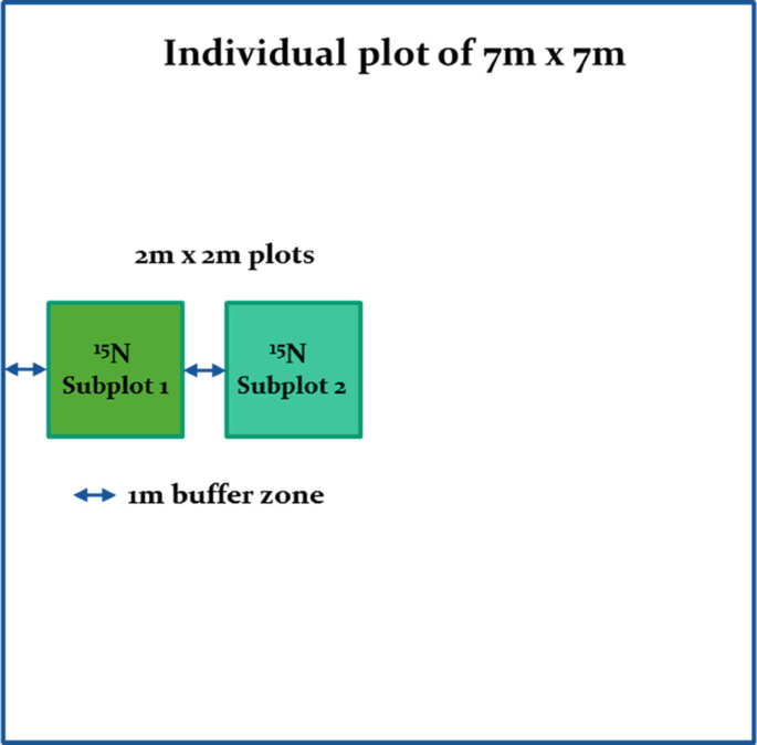

  

  Schematic diagram of the layout of the two sub-plots within a main plot, each with a 1 m buffer zone, each destined for ¹⁵N-labeled fertilizer application

• To ensure that no ¹⁵N-labeled fertilizer/residues are present from previous experiments, collect four soil cores (0–10 cm soil depth) from each of the two sub-plots, then combine them into one sample, and analyze for ¹⁵N content. This will establish the initial ¹⁵N level in the soil.

• Calculate the amount of ¹⁵N-labeled fertilizer (using a maximum of 5 atom % excess) to add to each 4 m² sub-plot using Eqs. 6.1 and 6.2. The amount of ¹⁵N-labeled urea at 40 kg N ha⁻¹ for a 4 m² sub-plot comes out to be 34.78 gram.

• Please note that if N fertilizer is applied in a single application, this 5 atom % excess could be reduced to 3 atom % excess (please refer to the dilution procedure at the end of this section).

• Separate the first sub-plot for ¹⁵N-labeled fertilizer by placing a temporary plastic sheet or any other similar material around the perimeter of the first sub-plot. Then, uniformly apply the required amount (0.39 kg) of ordinary urea to the entire (45 m²) of the larger main plot excluding the first sub-plot.

• After application of the ordinary urea, remove the plastic sheet around the first sub-plot, carefully weigh out the exact amount of ¹⁵N-labeled fertilizer (34.78 gram) using Eq. 6.2, and apply ¹⁵N-labeled urea evenly by hand to the first sub-plot. One shall be aware that ¹⁵N-labeled fertilizer such as urea come as a fine particle therefore extreme care shall be taken while applying to ensure its even application. Fine sand of the same diameter or any other inert material shall be mixed with the ¹⁵N-labelled urea to ensure even application. One shall also avoid ¹⁵N labelled urea under windy conditions or when a heavy rainfall is expected. If irrigation water is available, it is important that the experimental plots are supplied with at least 10–20 mm of irrigation soon after N fertilizer application to move urea from surface into the soil to minimize the risk of ammonia volatilization.

• When the time arrives for the 2nd split ¹⁵N fertilizer application, place a plastic sheet/cover around the perimeter of only the second sub-plot of 4 m² (this sub-plot will have previously received only ordinary urea) to ensure that ordinary urea is applied only to all areas of the main plot except the 2nd sub-plot during the 2nd fertilizer application. Then, uniformly apply the required amount (0.39 kg) of ordinary urea to the entire 45 m² of the larger main plot, but exclude the 2nd sub-plot.

• Remove the plastic sheet, and carefully apply the required amount (34.78 gram) of ¹⁵N-labeled fertilizer to the 2nd sub-plot as above.

• Carry out normal farm practices like spraying of herbicides and insecticides, and apply normal irrigation volumes until the wheat crop reaches its maturity.

• At the appropriate time, harvest the wheat crop from each sub-plot. For ¹⁵N uptake by below ground (roots) and aboveground plant parts (i.e., stems, leaves and grain), randomly select 3–4 wheat plants from the middle row of each sub-plot of ¹⁵N; and transfer them to plastic bags. After transporting wheat plant samples to the lab, separate the plant samples into (1) roots, (2) stem and leaves and (3) grain. Wash gently the plant tissue with tap water first, then with distilled water. After washing, allow water to drain and then dry the three types of wheat tissue samples at 65 °C for 7 days or until samples are dried to a constant weight.

• After drying, grind the wheat roots, leaves and stems and grain samples separately to a fine powder (for determination of the total N by Kjeldahl or by the combustion method). Then, accomplish the ¹⁵N determination by stable isotope mass spectrometry. Be certain to clean the grinder with a brush (and also use a blower), in between grinding the individual plant tissue samples.

• Also collect four soil samples (each 0–15 cm soil depth) from each of the two sub-plots; mix them to get one composite soil sample for ¹⁵N and total N analysis.

Wheat Straw and Grain Yield

• To determine wheat yield, select 3 m × 3 m area within each main-plot (7 m × 7 m) and harvest wheat crop at the same time as above for ¹⁵N analysis. Then, separate the biomass into (1) shoot and leaves and (2) grain and record their fresh bulk weight immediately.

  • [Note: Researchers must not use the small ¹⁵ N plot for biomass production]

• To determine moisture fraction in leaves plus stems (straw) and in grain, select 2 to 3 randomly chosen wheat plants, from each 3 m × 3 m plot; transfer them to plastic bags, seal each plastic bag using a rubber band to ensure that no water losses occur from the collected plant tissue. After transporting the wheat plant samples to the lab, separate the plant samples into straw and grain, and record their fresh weight. Wash them with tap water to remove the soil. Then take sub-tissue samples of each type of plant tissue (grain and straw), followed by drying the sub-samples of tissue at 65 °C for 7 days.

• Record the dry weights of the plant tissue after 7 days in order to calculate their moisture contents. This will provide the researcher with wheat dry matter yield (DM) per hectare as shown in Eq. (6.3).

  $$ \mathrm{Wheat}\ \mathrm{straw}\ \mathrm{or}\ \mathrm{grain}\ \mathrm{DM}\ \left(\mathrm{kg}\ \mathrm{per}\ \mathrm{ha}\right)=\mathrm{FB}\ \mathrm{Wt}\ \left(\mathrm{kg}\right)\times \frac{\mathrm{10,000}\ {\mathrm{m}}^2}{\mathrm{harvested}\ \mathrm{area}\ \left({\mathrm{m}}^2\right)}\times \frac{\mathrm{SD}\ \mathrm{Wt}\ \left(\mathrm{kg}\right)}{\mathrm{SF}\ \mathrm{Wt}\ \left(\mathrm{kg}\right)} $$

  (6.3)

Where, FB Wt is fresh bulk weight (kg per m²) of the harvested area of the sub-plot (area (3 m × 3 m), and SD Wt and SF Wt are sub-plot sample’s dry and fresh weights, respectively.

4.2 Calculation of Nitrogen Use Efficiency (NUE)

The following example provides step-by-step guidance for estimating fertilizer ‘N use efficiency’ of a wheat crop.

A field study was carried out with a wheat crop to assess the fertilizer N use efficiency of wheat grain which received nitrogen fertilizer at the rate of 80 kg N ha⁻¹ in 2 split doses (40 kg N ha⁻¹ for each of two application times). The experimental sub-plot was 4 m² in size and the ¹⁵N fertilizer was labeled with exactly 5% atom excess. At the end of growth period, assuming the grain yield from harvested wheat was 2667 kg per ha and the N content in the grain, as obtained by Kjeldahl analysis was 3.0%, the amount of total N removed from the soil by the wheat grain is calculated below (Eq. 6.4):

$$ \mathrm{Wheat}\ \mathrm{grain}\ \mathrm{N}\ \mathrm{uptake}\ \left(\mathrm{kg}\ \mathrm{N}\ \mathrm{per}\ \mathrm{ha}\right)=\frac{\mathrm{grain}\ \mathrm{yield}\ \left(\mathrm{kg}\ \mathrm{per}\ \mathrm{ha}\right)\times \mathrm{total}\ \mathrm{N}\ \left(\%\right)\ \mathrm{of}\ \mathrm{grain}}{100}\kern2.75em $$

(6.4)

$$ \mathrm{wheat}\ \mathrm{grain}\ \mathrm{N}\ \mathrm{uptake}=\frac{2667\times 3}{100}=80\ \mathrm{kg}\ \mathrm{N}\ \mathrm{per}\ \mathrm{ha} $$

The grain ¹⁵N measurements from the 1st and 2nd split applications of ¹⁵N-labeled fertilizers showed that an ‘atom excess percentage’ of 0.75% and 0.80% occurred, for the two sub-plots. The fertilizer N use efficiency of the grain is calculated as follows:

• (i) Percentage grain N derived from 1st and 2nd fertilizer application (% Ndff), based on the ratio of grain ¹⁵N [0.75% and 0.80%, to fertilizer ¹⁵N (5%)], can be calculated from Eq. 6.5.

$$ \% Ndff=\frac{{}^{15}{N}_{grain}}{{}^{15}{N}_{Fertilizer}}\times 100 $$

(6.5)

% Ndff for the 1st application = $\frac{0.75}{5}\times 100=15\%$

% Ndff for the 2nd application = $\frac{0.80}{5}\times 100=16\%$

% Ndff for the two split applications = 15 + 16 = 31%

• (ii) From the % Ndff, the amount of N derived from the two split fertilizer applications (Ndff) is calculated as:

$$ Ndff=\% Ndff\times \mathrm{N}\ \mathrm{taken}\ \mathrm{up}\ \mathrm{by}\ \mathrm{crop}\kern9.25em $$

(6.6)

$$ Ndff=\frac{31}{100}\times 80=24.8\ \mathrm{kg}\ \mathrm{N}\ \mathrm{per}\ \mathrm{ha} $$

[Note: The above equations (Eqs. 6.5 and 6.6) can also be used to calculate Ndff of the aboveground wheat plant tissues (straw) as well as roots, if such information is needed.]

Finally, fertilizer N use efficiency (FNUE) is calculated from Ndff (24.8) and N rate applied (80 kg N ha⁻¹).

$$ FNUE=\frac{Ndff}{\mathrm{Total}\ \mathrm{fertilizer}\ {\mathrm{N}}_{\mathrm{applied}}}\times 100 $$

(6.7)

$$ FNUE=\frac{24.8}{80}\times 100=31\% $$

Thus, in this study the wheat grain derived 31% of its N from the applied ¹⁵N-labeled urea fertilizer, with the remaining N (69%) coming from the pre-existing soil N pool.

4.3 An Example for ¹⁵N-Labeled Urea Dilution

For diluting 1 kg of ¹⁵N-labeled urea with 5 atom–3 atom %, please see the calculations below (Eq. 6.8) using a mixing model based on the following relationship:

$$ {f}_A+{f}_B=1 $$

(6.8)

Where, f_A and f_B refer to the fractions of labeled fertilizer and un-labeled fertilizers, respectively.

• First calculate the fraction of ¹⁵N-labeled fertilizer with 5 atom % (f_A) which will be required for mixing with un-labeled fertilizer to make 3 atom % using Eq. 6.9 below:

  $$ {f}_A=\frac{3-0.366}{5-0.366}=0.56841 $$

  (6.9)

• Then calculate the fraction of un-labeled fertilizer using Eq. (6.10) below:

  $$ {f}_B=1-0.5684=0.43159 $$

  (6.10)

Thus, for 1 kg of labeled fertilizer with 3 atom %, weigh 0.56841 kg of 5 atom % fertilizer and mix it with 0.43159 kg of un-labeled fertilizer.

5 Biological Nitrogen Fixation (BNF)

Over the past 62 years, world food supplies have become heavily dependent on the use of synthetic N fertilizers predominantly urea, with over half of this N fertilizer being applied to cereal crops. The use of fertilizer N will continue to play a critical role in ensuring world food security. Currently, world fertilizer N use is 113 million metric tons (2016), and this use is expected to increase to 120 million metric tons in 2018. Most of these increases in N fertilizer use will occur in developing countries.

Since the oil crisis of 1974 (and high N fertilizer prices), research attention of many international programs has focused on the use of biological N fixation (BNF) as an alternative N source in agro-ecosystems. Under this natural process, micro-organisms convert atmospheric N (N₂) into ammonia through enzymatic (nitrogenase) reactions for further utilization of the reduced N in plant metabolism. These N₂-fixing micro-organisms can live alone in the soil or in symbiosis with some plant species in a wide range of environments.

A classical example occurring in agricultural systems is the symbiotic association between Rhizobium bacteria and the roots of legumes in the Fabaceae family of plants (grain legumes, forage and pasture legumes and a number of tree species). Plant species in the Fabaceae are widely distributed in the world. In this symbiosis, the bacteria inoculate the roots of the legumes, and form nodules which are filled with bacteroids (an altered form of the bacteria).

Legume species are common sources of protein-rich food for humans and feed for their livestock, and they also provide fiber, medicines and other products. Grain legumes can be cultivated in a separate crop rotation, or by intercropping with cereals. The forage legume species are normally used in mixed swards. The tree legume species are employed in agro-forestry and agro-sylvo-pastoral systems. Certain fast-growing legume species may be included in cropping systems for use as cover crops, or incorporation into the soil as green manures.

In order to ensure appreciable biological nitrogen fixation (BNF) inputs into agricultural production systems, legume genotypes can be grown from seeds, or propagated vegetatively. Then, selected biofertilizers (commercially available Rhizobium cultures) are applied as inoculants to the seeds or seedlings, or to rooted cuttings for tree species. The amount of N₂ fixed by the legumes depends on the symbiosis established between the Rhizobium strain and the legume species. Here, the cultivar (genotype) as well as environmental (soil, climate) and agronomic management factors are also important. A number of stress conditions, such as salinity, acidity, drought, extreme temperatures and nutrient deficiencies have negative effects on both partners of the symbiosis.

Appreciable amounts of N₂ are fixed by legumes, thereby contributing to an improved soil fertility status and reducing the need for chemical fertilizer N. A significant proportion of this fixed N is utilized by the cereal crops or grasses which are grown in association with the legumes, or in a crop rotation with the legume. Other apparent benefits called ‘legume effects’, are also attributed to the inclusion of the legume into the agricultural system. Table 6.2 provides a summary of the legume’s effects in agro-ecosystems.

Table 6.2 Main effects of legumes in agro-ecosystem

Any program aimed at enhancing the use of legume BNF for improving soil fertility and crop productivity in cropping systems should include the ability to measure N₂ fixation under a wide range of environmental and agronomic management conditions. Methods to assess legume N₂ fixation under field conditions can be grouped into isotopic and non-isotopic methodologies.

5.1 Estimating Legume BNF Using ¹⁵N Isotope Techniques

Isotopic methods using the stable ¹⁵N isotope, both with enrichment and also at natural abundance levels, provide the most sensitive measures of total N₂ fixation over the growing cycle of legume crops. These are also the only methods capable of distinguishing atmospheric N₂ from other sources of N present in the soil.

Of the two main stable isotopes of N, the light isotope ¹⁴N, is by far the most abundant (99.6337%). The heavy stable isotope ¹⁵N, has an abundance of 0.3663 atom %. If the ¹⁵N concentrations within each of the two main sources of N (atmospheric N₂ and soil N) differ appreciably, then it is possible to calculate the proportion of the total N that accumulates within the legume tissues that is derived from atmospheric N₂ fixation.

When the aim is the assessment of the N input by N₂-fixing plants through BNF, three parameters are required: the content of N in plant material, the dry matter yield of the N₂-fixing plant and the percentage of N in the N₂-fixing plant derived from the atmosphere (%Ndfa). Considering these three parameters, it is possible to calculate the amount of N fixed, usually expressed in terms of kg N derived from BNF per ha, in field experiments, or mg N derived from BNF per plant or per pot in glasshouse experiments. Based on these estimates, it is also possible to calculate the amount of N derived from soil by discounting the amount of N derived from BNF from the total N.

The %Ndfa depends on the interaction between plant growth and efficiency of microsymbiont strain. It is also depends on the soil physical and chemical properties, (e.g., water and nutrient availability). The two most important isotopic techniques for this purpose are the ¹⁵N isotope dilution and ¹⁵N natural abundance technique (Boddey et al. 2000; Urquiaga et al. 2012; Collino et al. 2015). Other isotopic techniques, such as ¹⁵N₂ feeding and A-value can be also applied depending on the purpose of the BNF quantification, for which detailed procedures can be found in previous literature (e.g., IAEA 2001).

5.2 ¹⁵N Isotope Dilution Technique

The ¹⁵N isotope dilution technique has been the most applied isotopic technique for %Ndfa assessment. This technique is based on the dilution of soil N taken up by the N₂-fixing plant by N derived from air through BNF (Fig. 6.4). When this technique is applied it is assumed that the ¹⁵N enrichment of non N₂-fixing plant can be used as reference to assess the ¹⁵N enrichment of plant-available soil N (Fig. 6.4).

Fig. 6.4

Illustration of the ¹⁵N isotope dilution technique for the BNF quantification

To apply this technique, the soil N taken up by plants is labelled through application of ¹⁵N-enriched fertilizers. After the labelling, both N₂-fixing and non N₂-fixing reference plants are grown and sampled at the same time. In fact, if all N forms in soil were easily mineralisable and available for plant uptake, the direct ¹⁵N analysis of soil samples could be used as reference to assess ¹⁵N abundance of N fraction in N₂-fixing plants derived from soil. However, only the soil mineral N forms (mainly NH₄ ⁺ and NO₃ ⁻), representing a small fraction of N, is available for plant uptake and could theoretically be used to assess the ¹⁵N abundance of the N in plants derived from soil (Ledgard et al. 1984; Unkovich et al. 2008). Considering that non N₂-fixing plants has their N nutrition totally dependent on soil mineral N, these plants can be sampled to assess ¹⁵N enrichment of the plant-available soil N (Fig. 6.4). In this technique, N₂-fixing plant and the non N₂-fixing plant (reference) should have similar pattern of N uptake (Fig. 6.4). This is a critical prerequisite for application of ¹⁵N isotope dilution technique because, otherwise, the assessment of %Ndfa can be inaccurate when ¹⁵N enrichment of soil N is not constant in the time course and/or in the depths of soil N uptake by fixing and non-fixing plants (Baptista et al. 2014; Unkovich et al. 2008). Some procedures can be useful to deal with the non-constant ¹⁵N enrichment in time and soil depth, including the use of labile organic materials to immobilise excessive soil mineral N and stabilize N supply over time (Boddey et al. 1995) and constant addition of ¹⁵N-labelled fertiliser to the soil (Viera-Vargas et al. 1995). The %Ndfa by N₂-fixing plants is calculated using the following Eq. 6.11:

$$ \%\mathrm{Ndfa}=1-\frac{\mathrm{atom}\%{}^{15}\mathrm{N}\ {\mathrm{excess}}_{{\mathrm{N}}_2\mathrm{fixing}\ \mathrm{plant}}}{\mathrm{atom}\%{}^{15}\mathrm{N}\ {\mathrm{excess}}_{\mathrm{non}\ {\mathrm{N}}_2-\mathrm{fixing}\ \mathrm{reference}\ \mathrm{plant}}}\times 100 $$

(6.11)

The graphical representation of Eq. 6.11 is showed in Fig. 6.5. Taking in consideration that N fertiliser rate can impact the BNF process, it is usual to apply low N rates (e.g., <10 kg N ha⁻¹) when the objective is solely the labelling of plant-available soil N with ¹⁵N. When using low rates of N, fertiliser with high ¹⁵N enrichment is usually applied to yield plant materials with ¹⁵N/¹⁴N ratios adequate for precise and accurate analyses by spectrometry. The application of 1 kg of ¹⁵N excess per hectare (0.1 g ¹⁵N excess m⁻²) usually yields plant materials with sufficient ¹⁵N enrichment to be analysed with acceptable precision by most of mass spectrometers (emission spectrometers commonly requires higher ¹⁵N enrichments). Considering these values, if a rate of 10 kg N ha⁻¹ should be applied, the use of a fertiliser with 10 atom% ¹⁵N excess would be recommended. In fact, there is a possibility of using lower ¹⁵N enrichments depending on the spectrometer type, but this must be based on a rigorous assessment of analytical precision and after significant experience was gained. When this methodology is used for woody perennials, higher N rates (e.g., 20 kg N ha⁻¹) and/or ¹⁵N enrichments should be used.

Fig. 6.5

Relationship between ¹⁵N enrichment of N₂-fixing plant (abscissa axis) and percentage of N derived from atmosphere (%Ndfa, ordinate axis)

The selection of non N₂-fixing plants is a very important step for the accurate quantification of BNF by ¹⁵N isotope dilution technique. Some recommendations are presented below to avoid some biases due the selection of non N₂-fixing reference plants:

• To be sure that the reference plants do not have the ability of N₂-fixing, which could be identified by:

  • Classical N deficiency symptoms (e.g., pale green or yellow colour, especially in the older leaves).

  • Literature search indicating the inability of N₂-fixing. That is especially important for Poaceae, considering that some species of this plant family has the ability of N₂-fixing (Urquiaga et al. 1992; Reis et al. 2001).

  • Absence of nodules when non-nodulating isolines or non-inoculated legumes are used as reference plants.

• To use three or more reference plant species to assess the variability associated with the ¹⁵N enrichment of plant available soil N.

• Select non reference plants that presents patterns of N uptake similar to that of N₂-fixing plant, that is, have similar rooting depth and architecture exploiting the same pool of plant-available soil N and have the same dynamics of N uptake over time;

• If different varieties of a N₂-fixing crop having significant different life cycles are to be compared for the BNF ability, the group of varieties with similar life cycle must be paired with a reference plants with the duration of growth.

• Considering that differences in soil history can affect N mineralisation dynamics, additional reference plants must be grown and sampled for each different crop sequence even when BNF will be assessed for only one N₂-fixing crop type (e.g., effect of cropping history on BNF associated to soybean);

• Ideally, each reference plant should be considered as an additional treatment in the layout of field and glasshouse experiments, that is, they should be grown in additional field plots with the same replication and randomisation made for N₂-fixing crops.

To apply ¹⁵N-fertilisers aiming to label the plant-available soil N, the same strategy of ¹⁵N-microplot inside the main field plot previously described to study Fertilizer Use Efficiency can be used for BNF quantification using ¹⁵N isotope dilution technique. The plant material sampled in micro-plots will provide an estimate of %Ndfa. The dry matter yield, the total N taken up and the amount of N derived from BNF (e.g., kg N-BNF ha⁻¹) can be measured by harvesting larger area of the plot, including the area that received ¹⁴N-fertiliser.

5.3 Calculation of the Amount of N Derived from BNF by ¹⁵N Isotope Dilution Technique

The following example shows the steps for estimating the %Ndfa the amount of N derived from BNF, in kg N ha⁻¹, for soybean crop by ¹⁵N isotope dilution technique. A field study was carried out with a commercial soybean variety to assess the performance of three Rhizobium strains under a condition of water stress. The soybean was sown at row spacing of 0.50 m and three plant species were included as non N₂-fixing reference plants: Sorghum sp.; Brassica sp. and non-nodulating soybean. The quantification of BNF will be performed by ¹⁵N isotope dilution technique. Each experimental plot was 36 m² (6 m × 6 m). A micro-plot was established in an area of 9.0 m² (3.0 m × 3.0 m) in each experimental plot. For this study, ¹⁵N-labeled ammonium sulphate ((¹⁵NH₄)₂SO₄) with enrichments of 20 atom % ¹⁵N in excess was applied 50 days before sowing to each micro-plot at a rate of 5 kg N ha⁻¹. Non-labelled fertiliser ((¹⁴NH₄)₂SO₄) was also applied the remaining area of the plot. The soybean and reference plants were sown and harvested (105 days after sowing) concomitantly. The plants (shoot tissue) corresponding 1.5 m of the central row of the ¹⁵N-labelled micro-plot were collected, weighted, oven-dried, reweighted, ground and analysed for total N and ¹⁵N. Dry mass, N content and ¹⁵N-erichment are presented below (Table 6.3).

Table 6.3 Example of results of field experiment with soybean for quantification of BNF by ¹⁵N isotope dilution technique

The mean value of ¹⁵N enrichment of reference plants was 1.1305 atom % ¹⁵N excess. An example calculation for the soybean inoculated with strain A is presented as follows using Eqs. 6.12 and 6.13:

$$ \mathrm{Total}\ \mathrm{N}\ \mathrm{in}\ \mathrm{shoot}\ \left(\mathrm{kg}\ \mathrm{per}\ \mathrm{ha}\right)=\frac{\mathrm{Dry}\ \mathrm{mass}\ \left(\mathrm{kg}\ \mathrm{per}\ \mathrm{ha}\right)\times \mathrm{N}\ \mathrm{content}\ \left(\%\right)\ }{100} $$

(6.12)

$$ \mathrm{Total}\ \mathrm{N}\ \mathrm{in}\ \mathrm{shoot}=\frac{5097\times 3.7}{100}=189\ \mathrm{kg}\ \mathrm{N}\ \mathrm{per}\ \mathrm{ha} $$

$$ \%\mathrm{Ndfa}=1-\frac{\mathrm{atom}\%{}^{15}\mathrm{N}\ {\mathrm{excess}}_{{\mathrm{N}}_2\mathrm{fixing}\ \mathrm{plant}}}{\mathrm{atom}\%{}^{15}\mathrm{N}\ {\mathrm{excess}}_{\mathrm{non}\ {\mathrm{N}}_2-\mathrm{fixing}\ \mathrm{reference}\ \mathrm{plant}}}\times 100 $$

$$ \%\mathrm{Ndfa}=1-\frac{0.1420}{1.1305}\times 100=87\% $$

$$ \mathrm{Amount}\ \mathrm{of}\ \mathrm{N}\ \mathrm{derived}\ \mathrm{from}\ \mathrm{BNF}\ \left(\mathrm{kg}\ \mathrm{per}\ \mathrm{ha}\right)=\frac{\mathrm{Total}\ \mathrm{N}\ \mathrm{in}\ \mathrm{shoot}\ \left(\mathrm{kg}\ \mathrm{per}\ \mathrm{ha}\right)\times \%\mathrm{Ndfa}\ }{100} $$

(6.13)

$$ \mathrm{Amount}\ \mathrm{of}\ \mathrm{N}\ \mathrm{derived}\ \mathrm{from}\ \mathrm{BNF}=\frac{189\times 87\ }{100}=165\ \mathrm{kg}\ \mathrm{N}\ \mathrm{per}\ \mathrm{ha} $$

Considering the other data of shoot dry mass, N content and atom % ¹⁵N excess, the amounts of N derived from BNF for soybean inoculated with strain B was 184 kg N ha⁻¹ and for soybean inoculated with strain C was 106 kg N ha⁻¹.

5.4 ¹⁵N Natural Abundance Technique

This technique depends on the slight natural enrichment of ¹⁵N in the soil, relative to atmospheric N₂. The slight increase of ¹⁵N in soil is a consequence of the non- identical behaviour of the light and heavy isotopes involved in various reactions in the soil environment. The ¹⁵N isotopic fractionation, also called the mass discriminatory effect (Xing et al. 1997), is a result of complex and prolonged interaction of biological, chemical and physical processes in soils, which results in fractionation between ¹⁵N and ¹⁴N. There is a tendency of the reaction products, such as the gaseous N forms produced by denitrification, to become relatively enriched in the lighter isotope ¹⁴N, while the remaining N compounds, which can be stabilised in soil organic matter over time, tend to be enriched in the heavier isotope ¹⁵N (Xing et al. 1997). It is important to consider that this small ¹⁵N enrichment occurs in a long time scale, and is closely associated to soil organic matter retention and long-term dynamics (Ledgard et al. 1984).

Considering that ¹⁵N natural abundance technique is based on the analyses of plant samples having very small ¹⁵N deviation relative to atmospheric N₂, it is usual to express the results of ¹⁵N natural abundance analyses in terms of δ units. The δ¹⁵N value is the difference in the ratio ¹⁵N:¹⁴N of a given sample and the ratio ¹⁵N:¹⁴N in the nominated international standard of atmospheric N₂, expressed by parts per thousand (‰). One unit of δ¹⁵N (1.0‰) is a thousandth of the ¹⁵N natural abundance of the atmosphere (0.3663 atom% ¹⁵N) above or below the natural abundance of atmospheric N₂, that is, one unit of δ¹⁵N it is equal to 0.0003663 atom% ¹⁵N excess. The following Eq. 6.14 is applied to calculate the δ¹⁵N:

$$ \updelta {}^{15}\mathrm{N}\left({\mbox{\fontencoding{U}\fontfamily{wasy}\selectfont\char104}} \right)=\frac{\mathrm{atom}\%{}^{15}{\mathrm{N}}_{\mathrm{sample}}-\mathrm{atom}\%{}^{15}{\mathrm{N}}_{\mathrm{atmosphere}}}{\mathrm{atom}\%{}^{15}{\mathrm{N}}_{\mathrm{atmosphere}}}\times 1000 $$

(6.14)

Therefore, the δ¹⁵N of atmospheric N₂ will be by definition equal to 0‰. Positive value of δ¹⁵N means that there are an enrichment of ¹⁵N in the sample compared to the atmospheric N₂ and negative values means that the sample presents a slightly depletion. For example, if a plant sample has 0.35855 atom% ¹⁵N, the resulting δ¹⁵N of this sample is:

$$ \updelta {}^{15}\mathrm{N}=\frac{0.3659-0.3663}{0.3663}\times 1000=-1.09{\mbox{\fontencoding{U}\fontfamily{wasy}\selectfont\char104}} $$

The main advantage of the natural abundance technique, compared to ¹⁵N isotope dilution technique, is the no requirement to add ¹⁵N fertiliser to label the soil available N, which is a very expensive consumable and, depending on the N rates, it can affect BNF process. However, an important disadvantage of this technique is the need for an Isotope Ratio Mass Spectrometer with high precision.

The Eq. 6.15 can be used to calculate the Ndfa% by using the ¹⁵N natural abundance technique is:

$$ \mathrm{Ndfa}\%=\frac{\updelta\ {}^{15}{\mathrm{N}}_{\mathrm{reference}\ \mathrm{plant}}-\updelta\ {}^{15}{\mathrm{N}}_{\mathrm{fixing}\ \mathrm{plant}}}{\updelta\ {}^{15}{\mathrm{N}}_{\mathrm{reference}\ \mathrm{plant}} - B}\times 100 $$

(6.15)

where B is the δ¹⁵N for the N₂ fixing plant when completely dependent on N₂ fixation for growth. The B value is usually negative as a result of isotopic fractionation within the legume. The value of B depends on the plant species, plant age, symbiont and growth conditions. Unkovich et al. (2008) presented some tables with compilation of a wide number of B values for shoot of many tropical and temperate legumes, which can be used to estimate %Ndfa with an acceptable accuracy depending on the N₂ fixation level.

Another important factor affecting the %Ndfa estimate is the δ¹⁵N of the reference plant. The higher is this parameter, the better is the estimate of %Ndfa because this will result in less impact of biases associated to small variability of some processes, such as the mineralisation intensity of soil N pools, isotopic discrimination in plants or small differences in root architecture between N₂-fixing and non-fixing reference plants. Reference δ¹⁵N higher than 4‰ have been considered suitable for estimating %Ndfa in N₂-fixing plants (Unkovich et al. 2008).

An important practical procedure to have an initial estimate of ¹⁵N natural abundance of plant-available soil N before the beginning of the experiment is the ¹⁵N analysis of non N₂-fixing broadleaf and grass weeds in the experimental area available for BNF studies. Separated samples of the different reference plant should be collected in different points of the area to assess the variability of δ¹⁵N in plant-available N (not a composite sample). In addition to that, details on the history of the area are very useful, including previous crop type, N fertilisation (type and rates) and use of inoculants.

All recommendation presented for ¹⁵N isotope dilution technique to select non N₂-fixing plants must also be considered for the ¹⁵N natural abundance technique. The reference plants must be considered as additional treatments in the experimental design, with replication and randomisation. When experiments are conducted as randomised block design the %Ndfa estimate for the plants of a given block should be performed with the δ¹⁵N of the references of the same block individually.

Calculation of the Amount of N Derived from BNF by ¹⁵N Natural Abundance Technique

The following example shows the steps for estimating the %Ndfa and the amount of N derived from BNF, in kg N ha⁻¹, for common bean (Phaseolus vulgaris, L.) by ¹⁵N natural abundance technique:

A glasshouse study was carried out with two varieties of common bean to assess the osmotic effect of a salt (NaCl) on the BNF performance. The common bean cultivars and three reference plants (Sorghum sp.; Brassica sp. and non-nodulating bean) were sown in 10-L pots with 10 kg of soil. Three plants were used per each pot. Soil salinity was simulated by adding NaCl solution in soil. The BNF quantification will be performed by ¹⁵N natural abundance technique. The common bean shoots were collected at 60 days after sowing, weighted, oven-dried, reweighted, ground and analysed for total N and ¹⁵N. Dry mass, N content and ¹⁵N abundance are presented below (Table 6.4).

Table 6.4 Example of results of glasshouse experiment for measuring BNF associated to Phaseolus vulgaris by ¹⁵N natural abundance technique

The mean value of δ¹⁵N of reference plants was 9.82‰ and the B value used for common bean was −1.97‰. An example calculation for the variety A is presented as follows:

$$ \mathrm{Total}\ \mathrm{N}\ \mathrm{in}\ \mathrm{shoot}\ \left(\mathrm{g}\ \mathrm{per}\ \mathrm{pot}\right)=\frac{\mathrm{Dry}\ \mathrm{mass}\ \left(\mathrm{g}\ \mathrm{per}\ \mathrm{pot}\right)\times \mathrm{N}\ \mathrm{content}\ \left(\%\right)\ }{100} $$

$$ \mathrm{Total}\ \mathrm{N}\ \mathrm{in}\ \mathrm{shoot}=\frac{45\times 2.5}{100}=1.13\ \mathrm{g}\ \mathrm{N}\ \mathrm{per}\ \mathrm{pot} $$

$$ \mathrm{Ndfa}\%=\frac{\updelta\ {}^{15}{\mathrm{N}}_{\mathrm{reference}\ \mathrm{plant}}-\updelta\ {}^{15}{\mathrm{N}}_{\mathrm{fixing}\ \mathrm{plant}}}{\updelta\ {}^{15}{\mathrm{N}}_{\mathrm{reference}\ \mathrm{plant}} - B}\times 100 $$

$$ \mathrm{Ndfa}\%=\frac{9.82-0.52}{9.82-\left(-1.97\right)}\times 100=79\% $$

$$ \mathrm{Amount}\ \mathrm{of}\ \mathrm{N}\ \mathrm{derived}\ \mathrm{from}\ \mathrm{BNF}\ \left(\mathrm{mg}\ \mathrm{per}\ \mathrm{pot}\right)=\frac{\mathrm{Total}\ \mathrm{N}\ \mathrm{in}\ \mathrm{shoot}\ \left(\mathrm{g}\ \mathrm{per}\ \mathrm{pot}\right)\times \%\mathrm{Ndfa}\ }{100} $$

$$ \mathrm{Amount}\ \mathrm{of}\ \mathrm{N}\ \mathrm{derived}\ \mathrm{from}\ \mathrm{BNF}=\frac{1.13\times 79\ }{100}\times 1000=893\ \mathrm{mg}\ \mathrm{N}\ \mathrm{per}\ \mathrm{pot} $$

Considering the other data of shoot dry mass, N content and atom % ¹⁵N excess, the amounts of N derived from BNF for variety B was 761 mg N per pot.

5.5 Correction for N Derived from Seed

In some experiments using plants with proportionally large seeds or when plants are sampled in early growth stages, when N derived from seeds can supply a significant proportion of plant N, a correction in ¹⁵N enrichment/abundance of plant materials can improves the accuracy of the %Ndfa estimate (Okito et al. 2004). This correction is made by subtracting the amounts of N derived from seed and its ¹⁵N enrichment/abundance from plant material. For example, the following Eq. 6.16 is applied for correction when ¹⁵N natural abundance is applied:

$$ {\updelta}^{15}{\mathrm{N}}_{\mathrm{plant}\ \left(\mathrm{SC}\right)}=\frac{\left(\%{\mathrm{N}}_{\mathrm{plant}}\times {\mathrm{DM}}_{\mathrm{plant}}\times {\updelta}^{15}{\mathrm{N}}_{\mathrm{plant}}\right)-\left(\%{\mathrm{N}}_{\mathrm{s}\mathrm{eed}}\times {\mathrm{DM}}_{\mathrm{s}\mathrm{eed}}\times {\mathrm{P}}_{\mathrm{s}}\times {\updelta}^{15}{\mathrm{N}}_{\mathrm{s}\mathrm{eed}}\right)\ }{\left(\%{\mathrm{N}}_{\mathrm{plant}}\times {\mathrm{DM}}_{\mathrm{plant}}\right)-\left(\%{\mathrm{N}}_{\mathrm{s}\mathrm{eed}}\times {\mathrm{DM}}_{\mathrm{s}\mathrm{eed}}\right)} $$

(6.16)

where SC indicates the correction for seed N, %N is the N content, DM is the dry mass, P_s is the proportion of the seed N assimilated by plant tissue. P_s is usually assumed to be 0.5 when shoot tissue is analysed considering that half of N seed is incorporated in into the aerial tissue. The same equation can be applied for ¹⁵N isotope dilution technique by replacing the values of δ¹⁵N by atom% δ¹⁵N excess. When plants grown under field conditions and are sampled at the maturity stage this correction does not usually have a significant influence in the final estimate of %Ndfa because the contribution of seed N in this case is commonly small.

General Comments:

The use of ¹⁵N techniques has been successfully applied to measure BNF in many agricultural systems in many regions of the world. However, before the beginning of the experimentation using those isotope techniques it is important to take into account the main requirements needed for success in the BNF measurement: (i) the requirement of highly skilled workers for all activities from the selection of the experimental area to the interpretation of the ¹⁵N analysis, and (ii) the requirement of financial resources considering that consumables for ¹⁵N analysis are usually expensive compared to other routine plant and soil analyses. The selection of the most appropriate technique will depend mainly on the precision of the Mass-Spectrometer used for ¹⁵N analysis of plant materials. Other criteria are also presented in Table 6.5.

Table 6.5 Some advantages (A) and disadvantages (D) of two ¹⁵N isotope techniques for measuring BNF in agricultural systems

6 Water Stable Isotope Technique to Determine Evapotranspiration Partitioning

In agriculture, evapotranspiration (ET), or the flux of water from a vegetated surface via both evaporation (E) and transpiration (T) by plants, is an important component of the water budget. Water loss via transpiration can be considered ‘good’ water use, while water loss via evaporation can be considered ‘wasted’ water use (Fig. 6.6). Transpiration occurs through stomatal pores, the pores which are also used by the plants for uptake of atmospheric CO₂ in photosynthesis, and subsequent biosynthesis of carbon compounds, a process which ultimately leads to biomass gain. Stomata are tightly controlled by plant physiological signals to optimize carbon gain per unit of water lost. The use of the stable isotopes ¹⁸O and ²H as signatures in water and water vapor can help scientists to differentiate between water losses through direct soil evaporation versus transpiration from the plant leaves. That knowledge can be used to apply appropriate soil and water conservation strategies such as minimum tillage, mulching and a drip/spray irrigation system in order to minimize soil evaporation under a range of different management practices. Water use efficiency (WUE) of a plant species or crop type is related both to the plant’s genetics, as well as acclimation by the plant to the irrigation regime.

Fig. 6.6

Evapotranspiration model

Historically, the characterization of the plant processes involved in transpiration was performed through cumbersome and inaccurate water flux measurements. However, with the recent advancement of laser-based water vapor isotope analyzers, various calculation models have been developed to correlate the real-time, spatial, and temporal isotopic measurements with evaporation and transpiration fluxes (F_ET and F_T).

According to Yakir and Sternberg (2000), the ratio of these fluxes is calculated using Eq. 6.17:

$$ {f}_{T/ ET}=\frac{F_T}{F_{ET}}=\frac{\delta_{ET}-{\delta}_E}{\delta_T-{\delta}_E} $$

(6.17)

Where, δ _ET is the isotopic composition of bulk evapotranspiration, δ _E is the isotopic composition of evaporated soil-water, and δ _T is the isotopic composition of water transpired by the plant.

In this section, we demonstrate how laser-based absorption spectroscopy, and in particular, Cavity Ring-Down Spectroscopy (CRDS), can be applied to many steps of ET analyses, including: (i) characterization of partial pressure and the isotopic composition of the vertical water vapor profiles to determine the bulk ET signal through a Keeling mixing model, (ii) the use of soil water isotopic composition, in combination with the Craig-Gordon model, to determine the evaporation flux signature, and (iii) direct measurement of the isotopic signature of transpiration occurring in leaf chambers in order to determine the isotope signature of the water source.

6.1 Determining δ_ET Using the Keeling Mixing Model

6.1.1 Theory

The isotopic composition of an evapotranspiration flux can be determined by using the Keeling mixing model (1958), a model which correlates water concentration (C) and the isotopic composition (δ) of the mixed air above the surface (A), the background air (B), and the evapotranspiration flux (ET) Eq. 6.18.

Keeling Mixing Model

$$ {C}_A.{\delta}_A={C}_B.{\delta}_B+{C}_{ET}.{\delta}_{ET} $$

(6.18)

Assuming the concentration and the isotopic composition of the background air (C_B, δ_B) and evapotranspiration (C_ET, δ_ET) are constant over a short period of time, Eq. (6.18) can be rearranged so that δ_A is a function of 1/C_A. In this case, (Eq. 6.19) the intercept of a plot of 1/C_A (x-axis) versus δ_A (y-axis) will yield δ_ET.

$$ {\delta}_A=\left({\delta}_B-{\delta}_{ET}\right)\frac{C_B}{C_A}+{\delta}_{ET} $$

(6.19)

6.1.2 Experimental Approach

Experimentally, one can measure the isotopic composition of the mixed air, δ_Α, at various concentrations, C_A, by sampling the air at different elevations above the surface. The vertical profile provides the water concentration gradient which is required in order to determine δ_ET.

The procedure involves the following steps.

• Sample air above the soil surface at different heights. The heights at which you sample will depend on the specifics of the ecosystem being studied.

• Connect the sample lines to a manifold using a rotary valve selector.

• If possible, use a rotary valve which can be controlled via a Picarro water isotope analyzer. For example, the Picarro L2130-i or L2140-i , can be used to select the sample line through which air will be sent to the analyzer.

• Run the analyzer in dual mode: vapor and liquid measurement allows the analyzer to self-calibrate using a liquid water standard, while the vapor mode analyzes the sampled water vapor, thereby providing isotopic composition and concentration.

• Using the analyzer’s Dual Mode Coordinator, set the system to measure vapor from each sample port for 10 min (i.e., a total of 50 min for one cycle – please note 5 sampling heights in this example, Fig. 6.7). Measurements should be made at a frequency of 1 Hz.

  Fig. 6.7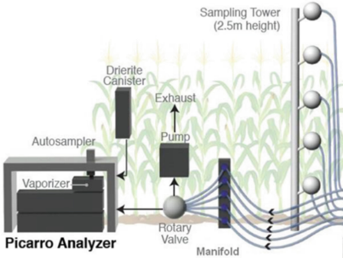

  

  Example of experimental setup for sampling water vapor at different heights

• It is recommended that the analyzer be calibrated with liquid water standards of a known isotopic composition once every 8 h. The auto-sampler injects the liquid standard sample into the vaporizer. Each injection measurement takes 9 min and a minimum of 6 injections for each liquid standard is required.

After the analyzer measurement, results are collected and processed (averaging and normalizing for each calibration), δ_A and 1/C_A are plotted on a graph as shown in the Fig. 6.8. Note that δ_ET is the y-intercept of the regression line between δ_A and 1/C_A.

Fig. 6.8

Example of a Keeling plot derived from a vertical profile of 5 water vapor measurements

6.2 Determining δ_ET Using the Craig-Gordon Model

6.2.1 Theory

The Craig-Gordon model (1965) is used to estimate the isotopic composition of soil-water evaporation. The model takes into account the effect of equilibrium and kinetic fractionations during the phase change between liquid to vapor (Eq. 6.20).

$$ {\delta}_E=\frac{\left({\delta}_L{\alpha}_e{h}_s-h{\prime}_A{\delta}_A\right)-\left({h}_s-{h}_s{\alpha}_e\right)-\left({\varepsilon}_k\right)}{\left({h}_s-h{\prime}_A\right)+{\varepsilon}_k} $$

(6.20)

Where, α_e is the equilibrium vapor-liquid fractionation factor. It can be calculated as a function of soil temperature, T_s, [K] as explained by Majoube (1971) (Eq. 6.21).

For ² H

$$ \ln {\alpha}_e=-52.612.{10}^{-3}+\frac{76.248}{T_s}-\frac{24.844.{10}^3}{T_s^2} $$

(6.21)

For ¹⁸O (Eq. 6.22 )

$$ \ln {\alpha}_e=2.0667.{10}^{-3}+\frac{0.4156}{T_s}-\frac{1.137.{10}^3}{T_s^2} $$

(6.22)

Where,

• δ_L is the soil liquid water isotopic composition [‰]

• δ_A is the ambient air water vapor isotopic composition [‰]

• h _s is the soil vapor saturation which is defined by Mathieu and Bariac (1996) (Eq. 6.23):

$$ {h}_s={e}^{M{\varphi}_s/R{T}_s} $$

(6.23)

• M is the molecular weight of water (18.0148 g/mol)

• φ _s is the soil potential (matric potential) of the evaporating surface [kPa]

• R is the ideal gas constant (8.3145 mL MPa/mol/K)

• T _s is the soil temperature, i.e. the temperature of the evaporating surface [K]

• ε_k is the kinetic isotopic fractionation factor (Eq. 6.24)

  $$ {\varepsilon}_k=n\left({h}_s-{h}_A^{\prime}\right)\left(1-\frac{D_i}{D}\right) $$

  (6.24)

• D _i /D, the ratio of molecular diffusion coefficients of water vapor in dry air, is taken as 0.9757 from Merlivat (1978) (Eq. 6.25):

$$ {h}_A^{\prime }=\frac{h_A{e}_{sA}}{a_w{e}_{s0}}\kern3.25em $$

(6.25)

• h′ _A is the humidity of the atmosphere normalized to the evaporating surface

• h _A is the humidity of the atmosphere

• e _sA and e _s0 are the saturation vapor pressures at the atmosphere’s (air’s) temperature and the temperature of the evaporation surface, respectively

• a _w is the thermodynamic activity of water

• n is related to the volumetric soil moisture (θ_s), the moisture of the residual (θ_res) and the saturated moisture (θ_sat), as proposed by Mathieu and Bariac (1996) (Eq. 6.26):

  $$ n=1-\frac{1}{2}\left(\frac{\theta_S-{\theta}_{res}}{\theta_{sat}-{\theta}_{res}}\right) $$

  (6.26)

6.2.2 Experimental Approach

Measuring δ_L

The isotopic composition of soil water will be measured using a Picarro water isotope analyzer (Fig. 6.9).

Fig. 6.9

Induction Module and Isotopic Water Analyzer

Several water extraction methods are available, as below:

Cryogenic Distillation

Cryogenic distillation is an established technique for extracting liquid water from samples, for example soils and leaves. Once extracted, the liquid water can be analyzed for its isotopic composition using a High Precision Vaporizer and Picarro water isotope analyzer.

Picarro Induction Module (IM)

The Picarro IM extracts water from soil samples by inductively heating the sample and directly sending the evaporated water vapor to the Cavity Ring-Down Spectroscopy (CRDS) analyzer. Prior to analysis on the CRDS, the water vapor is passed through a micro combustion cartridge to remove organic molecules which could potentially interfere with CRDS analysis. For more information about Picarro’s Induction Module, please visit:

• http://www.picarro.com/isotope_analyzers/im_crds.

When extracting water from soils using either of the above methods, caution should be applied to ensure that water extraction is complete. If water extraction is not complete, it is possible that fractionation may occur during isotopic analysis (or during the extraction process), which could then lead to inaccurate results. Care should also be taken during the storage of soil samples.

Measuring δ_A and C_A and Determining h_A

The isotopic composition of water vapor in the background ambient air is measured with the CRDS water analyzer when it is in the vapor mode.

Sample the ambient air well away from the studied system to ensure that no ‘local’ water vapor contamination occurs from evapotranspiration of the experimental plot, thereby affecting the ambient air measurement. This can be accomplished by placing the CRDS analyzer input port at an appreciable distance away from the experimental plot, or by connecting tubing to the inlet port of the CRDS in order to collect the air from well-above the canopy. The specific height above the canopy will be dependent on the ecosystem being studied.

Ensure that the CRDS analyzer is calibrated for isotopic composition and also the concentration dependence of the isotopic composition. For information on how to calibrate a Picarro Water Isotope Analyzer refer to the User’s Manual. A recent version is available at:

• https://picarro.box.com/s/0nh2wvm4n4ojf8jlmj7v.

The CRDS analyzer should be operated in dual mode: vapor and liquid. The liquid measurement allows the analyzer to calibrate itself with liquid standards. The vapor mode analyzes the sampled water vapor in ambient air to provide isotopic composition δ_A and concentration C _A.

Calculate h _A using C _A.

6.3 Determining δ_T via Direct Measurement at the Leaf

6.3.1 Theory

When re-arranging the mass balance established in Eq. 6.18, we get (Wang et al. 2012):

$$ {\delta}_T=\frac{C_M{\delta}_M-{C}_A{\delta}_A}{C_M-{C}_A} $$

(6.27)

Where, δ_A and C_A are the isotopic composition and water concentration of the ambient air; δ_M and C_M are the isotopic composition and water concentration measured from the leaf chamber, i.e. where transpiration water vapor mixes with ambient air.

6.3.2 Experimental Approach

Measuring δ_A and C_A

Follow exactly the procedure described on the previous page. One can directly measure the isotopic composition of the mixed air, δ _M and water concentration, C _M, inside of the leaf chamber. Figure 6.10 depicts the experimental setup:

• A leaf chamber is typically made of transparent plastic with a variable internal volume which will be dependent on the leaf size. The chamber has two small air vents to allow ambient air to flow into the chamber and mix with the water vapor generated by transpiration from the leaf.

• A 1/8-inch ID Teflon tubing connects the leaf chamber to the analyzer.

• Place a leaf, which remains attached to the plant, into the leaf chamber.

• Ensure that the CRDS analyzer is calibrated for isotopic composition and concentration dependence of the isotopic composition. For information on how to calibrate the Picarro Water Isotope Analyzer refer to the User’s Manual. A recent version is available at:

  https://picarro.box.com/s/0nh2wvm4n4ojf8jlmj7v.

• As detailed previously, operate the analyzer in the dual measurement mode: liquid and vapor. The liquid measurement allows the analyzer to calibrate itself with a liquid water standard while the vapor mode analyzes the sampled water vapor to provide isotopic composition and concentration.

Fig. 6.10

Experimental setup for measuring δ _M and C _M

7 Application of Other Isotopes

As mentioned in earlier sections of this chapter, nuclear and isotopic techniques have a wide range of applications in the soil-water-plant interaction studies, covering the fields such as plant ecology, physiology, biochemistry, nutrition, microbiology, protection against insect pests, and soil fertility, chemistry, physics, and hydrology, etc. Few common examples of the applications of isotopic and nuclear techniques in agricultural research are listed below.

• ³²P fertilizer use efficiency, root activity, DNA probes in molecular biology

• ³⁵S in soil and fertilizer studies

• ⁶⁵Zn in plant uptake and use efficiency

• ¹³C, ¹⁴C in soil organic matter dynamics, root activity, photosynthesis, pesticide residues, water use efficiency, etc.

• ²²Na, ³⁶Cl, ⁴⁰K in ion uptake and mechanism of salt tolerance in plants

• ¹³⁷Cs in soil erosion studies

• ⁶⁰Co for sterile insects in integrated pest management (IPM)

• ¹⁹⁸Gold-198 for detection of termite colonies in agricultural fields

The nuclear and isotopic techniques are the supporting tools, and not substitute, to the conventional techniques for understanding the biological processes and mechanisms of ecosystem functioning. Therefore, a careful evaluation is required with regard to: i) the need for using an isotopic/nuclear technique, and ii) the choice of the appropriate isotopic/nuclear considering the research objective, facilities and expertise available, risks involved in safe handling and disposal of hazardous materials, and the financial considerations. In this context, the stable isotopes are the ever preferred choice in soil-water-plant-atmosphere studies. Thus, examples and protocols of using ¹⁵N, ¹⁸O and ²H in plant nutrient and water use efficiency studies have been elaborated in this chapter. The reader is, however, referred to the IAEA Training Manuals (IAEA 1990, 2001) and the review by Nguyen et al. (2011), may one need further details.

References

Baptista RB, Moraes RF, Leite JM, Schultz N, Alves BJR, Boddey RM, Urquiaga S (2014) Variations in the 15N natural abundance of plant-available N with soil depth: their influence on estimates of contributions of biological N2 fixation to sugarcane. Appl Soil Ecol 73:124–129
Boddey RM, Oliveira OC, Alves BJR, Urquiaga S (1995) Field application of the 15N isotope dilution technique for the reliable quantification of plant-associated biological nitrogen fixation. Fertil Res 42:77–87
Boddey RM, Peoples MB, Palmer B, Dart PJ (2000) Use of the 15N natural abundance technique to quantify biological nitrogen fixation by woody perennials. Nutr Cycl Agroecosyst 57(3):235–270
Collino DJ, Salvagiotti F, Perticari A, Piccinetti C, Ovando G, Urquiaga S, Racca RW (2015) Biological nitrogen fixation in soybean in Argentina: relationships with crop, soil, and meteorological factors. Plant Soil 392(1–2):239–252
Craig H, Gordon L (1965) Deuterium and oxygen-18 variations in the ocean and the marine atmosphere. In: Stable isotopopes in oceanographic studies and paleotemperatures. Laboratorio Di Geologica Nucleare, Pisa, pp 9–130
IAEA (1990) Use of nuclear techniques in studies of soil-plant relationships. Training course series no 2 (Hardarson G, ed). International Atomic Energy Agency, Vienna, Austria, 223 pp
IAEA (2001) Use of isotope and radiation methods in soil and water management and crop nutrition – Training Course Series No. 14. International Atomic Energy Agency, Vienna, Austria, 247 pp
Keeling C (1958) The concentration and isotopic abundances of atmospheric carbon dioxide in rurals. Geochimica et Cosmochimica Acta 13(4):322–324
Ledgard SF, Freney JR, Simpson JR (1984) Variations in natural enrichment of 15N in the profiles of some Australian pasture soils. Soil Res 22:155–164
Majoube M (1971) Fractionnement en oxygene-18 et en deuterium entre l’eau et sa vapeur. J Chim Phys Biol 68:1423–1436
Mathieu R, Bariac T (1996) A numerical model for the simulation of stable isotope profiles in drying soils. J Geophys Res 101(D7):12685–12696
Merlivat L (1978) Molecular diffusivities of H2 16O, HD16O, and H2 18O in gases. J Chem Phys 69:2864–2871
Nguyen ML, Zapata F, Lal R, Dercon G (2011) Role of isotopic and nuclear techniques in sustainable land management: achieving food security and mitigating impacts of climate change. In: Lal R, Stewart BA (eds) World soil resources and food security, advances in soil science, vol 18. CRC Press, Boca Raton, pp 345–418
Okito A, Alves BRJ, Urquiaga S, Boddey RM (2004) Isotopic fractionation during N2 fixation by four tropical legumes. Soil Biol Biochem 36(7):1179–1190
Peoples MB, Faizah AW, Rerkasem B, Herridge DF (1989) Methods of evaluating nitrogen fixation by nodulated legumes in the field, ACIAR Monograpg No 11. ACIAR, Canberra, 76 pp
Pessarakli M (1991) Dry matter nitrogen-15 absorption and water uptake by green beans under sodium chloride stress. Crop Science 31:1633–1640
Reis VM, Reis FB Jr, Quesada DM, Oliveira OC, BJR A, Urquiaga S, Boddey RM (2001) Biological nitrogen fixation associated with tropical pasture grasses. Funct Plant Biol 28(9):837–844
Saranga Y, Menz M, Jiang CX, Robert WJ, Yakir D, Andrew HP (2001) Genomic dissection of genotype X environment interactions conferring adaptation of cotton to arid conditions. Genome Res 11:1988–1995
Unkovich M, Herridge D, Peoples M, Cadisch G, Boddey RM, Giller K, Alves BJR, Chalk P (2008) Measuring plant-associated nitrogen fixation in agricultural systems, ACIAR Monograph no 136. Australian Centre for International Agricultural Research, Canberra, p 258
Unkovich MJ, Pate JS (2000) An appraisal of recent field measurements of symbiotic N2 fixation by annual legumes. Field Crops Res 65(2):211–228
Urquiaga S, Cruz KHS, Boddey RM (1992) Contribution of nitrogen fixation to sugar cane: nitrogen-15 and nitrogen balance estimates. Soil Sci Soc Am J 56:105–114
Urquiaga S, Xavier RP, Morais RF, Batista RB, Schultz N, Leite JM, Sá JME, Barbosa KP, Resende AS, Alves BJR, Boddey RM (2012) Evidence from field nitrogen balance and 15N natural abundance data for the contribution of biological N2 fixation to Brazilian sugarcane varieties. Plant Soil 356:5–21
Viera-Vargas MS, Oliveira OC, Souto CM, Cadisch G, Urquiaga S, Boddey RM (1995) Use of different 15N labelling techniques to quantify the contribution of biological N2 fixation to legumes. Soil Biol Biochem 27(9):1185–1192
Wang L, Good S, Caylor K, Cernusak L (2012) Direct quantification of leaf transpiration isotopic composition. Agric For Meteorol 154–155:127–134
Witty JF, Renne RJ, Atkins CA (1988) 15N addition methods for assessing N2 fixation under field conditions. In: Summerfield RJ (ed) World crops: cool season food legumes. Kluwer Academic, Dordrecht, pp 716–730
Xing GX, Cao YC, Sun GQ (1997) Natural 15N abundance in soils. In: Zhu ZL, Wen Q, Freney JR (eds) Nitrogen in soils of China. Kluwer Academic, London, pp 31–41
Yakir D, Sternberg L (2000) The use of stable isotopes to study ecosystem gas exchange. Oecologica 123(3):297–311
Zaman M, Zaman S, Adhinarayanan C, Nguyen ML, Nawaz S (2013b) Effects of urease and nitrification inhibitors on the efficient use of urea for pastoral systems. Soil Sci Plant Nutr 59:649–659
Zaman M, Saggar S, Stafford AD (2013a) Mitigation of ammonia losses from urea applied to a pastoral system: the effect of nBTPT and timing and amount of irrigation. N Z Grassl Assoc 75:121–126
Zaman M, Barbour MM, Turnbull MH, Kurepin LV (2014) Influence of fine particle suspension of urea and urease inhibitor on nitrogen and water use efficiency in grassland using nuclear techniques. In: Heng LK, Sakadeva K, Dercon G, Nguyen ML (eds) International Symposium on managing soils for food security and climate change adaption and mitigation. Food and Agriculture Organization of the United Nations, Rome, pp 29–32
Author information
Authors and Affiliations
Corresponding author
Rights and permissions
The opinions expressed in this chapter are those of the author(s) and do not necessarily reflect the views of the IAEA, its Board of Directors, or the countries they represent
Open Access This chapter is licensed under the terms of the Creative Commons Attribution 3.0 IGO License (https://creativecommons.org/licenses/by/3.0/igo/), which permits use, sharing, adaptation, distribution and reproduction in any medium or format, as long as you give appropriate credit to the IAEA, provide a link to the Creative Commons licence and indicate if changes were made.
The use of the IAEA's name, and the use of the IAEA's logo, shall be subject to a separate written licence agreement between the IAEA and the user and is not authorized as part of this CC-IGO licence. Note that the link provided above includes additional terms and conditions of the licence.
The images or other third party material in this chapter are included in the chapter's Creative Commons licence, unless indicated otherwise in a credit line to the material. If material is not included in the chapter's Creative Commons licence and your intended use is not permitted by statutory regulation or exceeds the permitted use, you will need to obtain permission directly from the copyright holder.
Copyright information
© 2018 International Atomic Energy Agency
About this chapter
Cite this chapter
Zaman, M., Shahid, S.A., Heng, L. (2018). The Role of Nuclear Techniques in Biosaline Agriculture. In: Guideline for Salinity Assessment, Mitigation and Adaptation Using Nuclear and Related Techniques . Springer, Cham. https://doi.org/10.1007/978-3-319-96190-3_6
Download citation
DOI: https://doi.org/10.1007/978-3-319-96190-3_6
Published:
Publisher Name: Springer, Cham
Print ISBN: 978-3-319-96189-7
Online ISBN: 978-3-319-96190-3
eBook Packages: Earth and Environmental ScienceEarth and Environmental Science (R0)