Introduction to Soil Salinity, Sodicity and Diagnostics Techniques

Abstract

It is widely recognized that soil salinity has increased over time. It is also triggered with the impact of climate change. For sustainable management of soil salinity, it is essential to diagnose it properly prior to take proper intervention measures. In this chapter soil salinity (dryland and secondary) and sodicity concepts have been introduced to make it easier for readers. A hypothetical soil salinity development cycle has been presented. Causes of soil salinization and its damages, socio-economic and environmental impacts, and visual indicators of soil salinization and sodicity have been reported. A new relationship between ECe (mS/cm) and total soluble salts (meq/l) established on UAE soils has been reported which is different to that established by US Salinity Laboratory Staff in the year 1954, suggesting the latter is specific to US soils, therefore, other countries should establish similar relationships based on their local conditions. Procedures for field assessment of soil salinity and sodicity are described and factors to convert EC of different soil:water (1:1, 1:2.5 & 1:5) suspensions to ECe from different regions are tabulated and hence providing useful information to those adopting such procedures. Diversified salinity assessment, mapping and monitoring methods, such as conventional (field and laboratory) and modern (electromagnetic-EM38, optical-thin section and electron microscopy, geostatistics-kriging, remote sensing and GIS, automatic dynamics salinity logging system) have been used and results are reported providing comprehensive information for selection of suitable methods by potential users. Globally accepted soil salinity classification systems such as US Salinity Lab Staff and FAO-UNESCO have been included.

Keywords

1 Introduction

Soil is a non-renewable resource; once lost, can’t be recovered in a human lifespan. Soil salinity, the second major cause of land degradation after soil erosion, has been a cause of decline in agricultural societies for 10,000 years. Globally about 2000 ha of arable land is lost to production every day due to salinization. Salinization can cause yield decreases of 10–25% for many crops and may prevent cropping altogether when it is severe and lead to desertification. Addressing soil salinization through improved soil, water and crop management practices is important for achieving food security and to avoid desertification.

1.1 What Is Soil Salinity?

Soil salinity is a measure of the concentration of all the soluble salts in soil water, and is usually expressed as electrical conductivity (EC). The major soluble mineral salts are the cations: sodium (Na⁺), calcium (Ca²⁺), magnesium (Mg²⁺), potassium (K⁺) and the anions: chloride (Cl⁻), sulfate (SO₄ ²⁻), bicarbonate (HCO₃ ⁻), carbonate (CO₃ ²⁻), and nitrate (NO₃ ⁻). Hyper-saline soil water may also contain boron (B), selenium (Se), strontium (Sr), lithium (Li), silica (Si), rubidium (Rb), fluorine (F), molybdenum (Mo), manganese (Mn), barium (Ba), and aluminum (Al), some of which can be toxic to plants and animals (Tanji 1990).

From the point of view of defining saline soils, when the electrical conductivity of a soil extract from a saturated paste (ECe) equals, or exceeds 4 deci Siemens per meter (dS m⁻¹) at 25 °C, the soil is said to be saline (USSL Staff 1954), and this definition remains in the latest glossary of soil science in the USA.

1.1.1 Units of Soil Salinity

Salinity is generally expressed as total dissolved solutes (TDS) in milli gram per liter (mg l⁻¹) or parts per million (ppm). It can also be expressed as total soluble salts (TSS) in milli equivalents per liter (meq l⁻¹).

The salinity (EC) was originally measured as milli mhos per cm (mmho cm⁻¹), an old unit which is now obsolete. Soil Science has now adopted the Systeme International d’Unites (known as SI units) in which mho has been replaced by Siemens (S). Currently used SI units for EC are:

• milli Siemens per centimeter (mS cm⁻¹) or

• deci Siemens per meter (dS m⁻¹)

The units can be presented as:

1 mmho cm⁻¹ = 1 dS m⁻¹ = 1 mS cm⁻¹ = 1000 micro Siemens per cm (1000 μS cm⁻¹)

• EC readings are usually taken and reported at a standard temperature of 25 °C.

• For accurate results, EC meter should be checked with 0.01 N solution of KCl, which should give a reading of 1.413 dS m⁻¹ at 25 °C.

No fixed relationship exists between TDS and EC, although a factor of 640 is commonly used to convert EC (dS m⁻¹) to approximate TDS. For highly concentrated solutions, a factor of 800 is used to account for the suppressed ionization effect on EC.

Similarly, no one relationship exists between ECe and total soluble salts (TSS), although a factor of 10 is used to convert ECe (dS m⁻¹) to TSS (expressed in meq l⁻¹) in the EC range of 0.1–5 dS m⁻¹ (USSL Staff 1954). One relationship between ECe and TSS is presented in the Agriculture Handbook 60 (USSL Staff 1954). This relationship was developed using USA soils and has been widely used (worldwide) for over six decades. No efforts have been made to validate this relationship in other soils, though recently Shahid et al. (2013) have published a similar relationship for sandy desert soils ranging from low salinity (desert sand) to hyper-saline soils (coastal lands) in the Abu Dhabi Emirate. This latter work established a relationship between ECe and TSS which differs significantly from that of USSL Staff (1954), thus, opening the way for other countries to develop country-specific relationships which will allow better prediction and management of their saline and saline-sodic soils.

1.1.2 Why Total Soluble Salts Versus ECe Relationship Is Required?

Laboratories in some developing countries do not generally have modern equipment, i.e. flame emission spectrophotometer (FES), atomic absorption spectrophotometer (AAS), or inductively coupled plasma (ICP) in order to analyze soil saturation extracts or water samples for soluble Na⁺ to determine sodicity (sodium adsorption ratio – SAR). In contrast, Ca²⁺ and Mg²⁺ are easy to measure using a titration method, one which does not require modern instruments. Currently, these laboratories in many developing countries determine soluble Na⁺ by calculating the difference between the total soluble salts (TSS) and the quantities of Ca²⁺ + Mg²⁺ in order to make the analyses affordable, as below:

$$ {\mathbf{Na}}^{+}=\left[\left(\ \mathbf{Total}\ \mathbf{soulble}\ \mathbf{salts}\right)\ \mathbf{minus}\ \left({\mathbf{Ca}}^{\mathbf{2}+}+{\mathbf{Mg}}^{\mathbf{2}+}\right)\right] $$

The TSS are recorded from a graph [see Fig. 4, page 12 of the Agriculture Handbook 60 (USSL Staff 1954)] by using the ECe value (Fig. 1.1). The Na⁺ amount is then used to determine SAR so that exchangeable sodium percentage (ESP) can be calculated as:

Fig. 1.1

Relationship between total soluble salts (TSS) on y-axis and ECe on x-axis. (Source: Fig. 4, page 12, Agriculture Handbook 60 (USSL Staff 1954))

$$ \mathrm{SAR}=\frac{{\mathrm{Na}}^{+}}{\sqrt{\frac{1}{2}\ \left({\mathrm{Ca}}^{2+}+{\mathrm{Mg}}^{2+}\right)}} $$

$$ \mathrm{ESP}=\frac{\left[100\ \left(-0.0126+0.01475\times \mathrm{SAR}\right)\right]}{\left[1+\left(-0.0126+0.01475\times \mathrm{SAR}\right)\right]} $$

Where, each of Na⁺, Ca²⁺ + Mg²⁺ concentrations are expressed in milli equivalents per liter (meq l⁻¹) and SAR is expressed as (milli moles per liter)^0.5 (mmoles l⁻¹)^0.5.

In the above method of determining Na⁺ by calculating the difference between TSS and Ca²⁺ + Mg²⁺, any K⁺ amounts present are added to the Na⁺ (which is thus overestimated). It should be noted that the TSS versus ECe curve developed by USSL Staff (1954) was developed for the Western North American soils and, thus, may or may not be representative of soils of other countries. Hence, using such a practice may lead one to overestimate the sodicity hazard in irrigation waters or in saturation extracts of soils. This could lead to incorrect predictions and the use of inappropriate management options.

The finding of Shahid et al. (2013) has revealed an appreciable difference between the straight line (TSS versus ECe) determined from USSL Staff (1954) relative to protocols established by Shahid et al. (2013), shown in Figs. 1.1 and 1.2.

Fig. 1.2

Relationship between TSS and ECe (from Shahid et al. 2013)

The TSS/ECe ratio, thus, ranges between 10 (at ECe 1 dS m⁻¹) and 16 (at ECe 200 dS m⁻¹) based on USSL Staff (1954) relationship (Fig. 1.1). In contrast, use of the relationship obtained from the methods developed by Shahid et al. (2013), the TSS/ECe ratio ranged between 10 (at 1 dS m⁻¹), 11.38 (at ECe 200 dS m⁻¹) and 12 (at ECe 500 dS m⁻¹). A comparative representation is shown in Figs. 1.3 and 1.4.

Fig. 1.3

A comparison of the relationship between total soluble salts (TSS)/ECe established using the Agriculture Handbook 60 curve (USSL Staff 1954) for the soils of Abu Dhabi Emirate and the relationship established for the same soils by the ICBA/EAD curve (Shahid et al. 2013)

Fig. 1.4

Average lines showing the relationship between ECe and total soluble salts (TSS) from the USSL method (line from Fig. 1.1, above) for the soils of Abu Dhabi Emirate using the method developed by Shahid et al. (2013) using the average line adapted from Fig. 1.2, above

In order to test the above lines to determine soil sodicity, Shahid et al. (2013) gave three examples using one soil type, as below.

Example 1

Determination of sodium adsorption ratio (SAR) accomplished by analyzing soil saturation extract for ECe (using an EC meter), and soluble Na⁺, Ca²⁺, Mg²⁺ determined by using an atomic absorption spectrophotometer.

ECe:

= 51 dS m⁻¹

Soluble Na⁺:

= 480 meq l⁻¹

Ca²⁺:

= 50 meq l⁻¹

Mg²⁺:

= 38 meq l⁻¹

SAR:

= 72.4 (mmoles l⁻¹)^0.5

Example 2

Determination of sodium adsorption ratio (SAR) accomplished by analyzing soil saturation extract for ECe (using an EC meter), soluble Ca²⁺ and Mg²⁺ (by titration procedure) and soluble Na⁺ estimated by calculating the difference between TSS and Ca²⁺ + Mg²⁺ using USSL Staff (1954) relationship (Fig. 1.1).

ECe:

= 51 dS m⁻¹

TSS:

= 720 meq l⁻¹ (from Fig. 1.1)

Soluble Na⁺:

= 632 meq l⁻¹ (by difference, i.e. 720–88 = 632)

Ca²⁺:

= 50 meq l⁻¹

Mg²⁺:

= 38 meq l⁻¹

SAR:

= 95.32 (mmoles l⁻¹)^0.5

Example 3

Determination of sodium adsorption ratio (SAR) accomplished by analyzing soil saturation extract for ECe (using an EC meter), soluble Ca²⁺ and Mg²⁺ (by titration procedure) and soluble Na⁺ by calculating the difference using the relationship developed by Shahid et al. (2013) (Fig. 1.2).

ECe:

= 51 dS m⁻¹

TSS:

= 560 meq l⁻¹ (from Fig. 1.2)

Soluble Na⁺:

= 472 meq l⁻¹ (by difference, i.e. 560–88 = 472)

Ca²⁺:

= 50 meq l⁻¹

Mg²⁺:

= 38 meq l⁻¹

SAR:

= 71.2 (mmoles l⁻¹)^0.5

The above three examples clearly show that the SAR (71.2) when determined by using the Shahid et al. (2013) relationship (Fig. 1.2) is very close to the SAR determined by analyzing the saturation extract by modern laboratory equipment (71.2 versus 72.4). However, when SAR was determined by using the USSL Staff (1954) relationship, it was appreciably higher (95.32) than the SAR values determined by other procedures.

This indicates that the Na⁺ value obtained by using the USSL Staff (1954) relationship can lead to higher SAR and can, thus, mislead the sodicity prediction. The above examples have confirmed that the relationship established for the soils of Abu Dhabi Emirate by Shahid et al. (2013) can be used reliably to determine soil sodicity (SAR and ESP). Thus, the analyses become rapid and affordable for the use in developing countries. Also of importance is the need for developing countries, e.g. the Gulf Cooperation Council (GCC) and ARASIA countries, who are relying on the USSL Staff (1954) curve to determine soluble sodium by calculating the difference between TSS and Ca²⁺ + Mg²⁺, to validate this relationship for local soils.

2 Causes of Soil Salinity

There can be many causes of salts in soils; the most common sources (Plate 1.1) are listed below:

• Inherent soil salinity (weathering of rocks, parent material)

• Brackish and saline irrigation water (Box 1.1)

• Sea water intrusion into coastal lands as well as into the aquifer due to over extraction and overuse of fresh water

• Restricted drainage and a rising water-table

• Surface evaporation and plant transpiration

• Sea water sprays, condensed vapors which fall onto the soil as rainfall

• Wind borne salts yielding saline fields

• Overuse of fertilizers (chemical and farm manures)

• Use of soil amendments (lime and gypsum)

• Use of sewage sludge and/or treated sewage effluent

• Dumping of industrial brine onto the soil

Plate 1.1

Soil salinity development in agriculture and coastal fields. (a) Salinity in a furrow irrigated barley field, (b) Salinity in a sprinkler irrigated grass field, (c) Salinity due to sea water intrusion in coastal land

Box 1.1: Salt Loads in Soil Due to Irrigation

It is generally believed that irrigation with fresh water is safe for optimum crop production; this may be true for short duration. However, if this water is used over a long period without managing for salinity, a significant quantity of salts will be added into soil. A simple example is given below.

Assume that fresh water (EC 0.2 dS m⁻¹) is used for irrigating the crop and 8500 cubic meters per hectare (850 mm) of this water is used over the entire crop season. The water of EC 0.2 dS m⁻¹ contains approximately 128 mg l⁻¹ salts (0.2 × 640) which are equivalent to 0.128 kg per cubic meter of irrigation water. Over the crop season, 1088 kg of salts will, thus, be added to each hectare with the irrigation water. If we assume that the dry matter harvested from each hectare is about 15 metric tons, and there is 3.5% by weight of total salts in the harvested crop biomass, then the portion of salt harvested with the crop is 525 kg. This leaves 563 kg of salts in the soil directly or in the plant parts (belowground, stubbles, debris) which will be returned to the soil by cultivation and subsequent decay of the plant biomass left in the field. This example is a very conservative one. It is more likely that water of a higher salinity will be used for irrigation. Thus, a salinity management program needs to be implemented for virtually all irrigated agricultural crops, especially those growing in low natural rainfall areas.

3 Salinity Development in Soils – A Hypothetical Cycle

Recently Shahid et al. (2010) have hypothesized a soil salinity cycle in order to present various facets in the development of soil salinity (Fig. 1.5).

Fig. 1.5

A hypothetical soil salinization cycle. (Adapted from Shahid et al. 2010)

4 Types of Soil Salinity

4.1 Dryland Soil Salinity

Salinity in dryland soils develops through a rising water table and the subsequent evaporation of the soil water. There are many causes of the rising water table, e.g. restricted drainage due to an impermeable layer, and when deep-rooted trees are replaced with shallow-rooted annual crops. Under such conditions, the groundwater dissolves salts embedded in rocks in the soil, with the salty water eventually reaching the soil surface, and evaporating to cause salinity. Dryland salinity can also occur in un-irrigated landscapes. There are no quick fixes to dryland salinity, though modern technologies in assessment and monitoring can allow one to follow and better understand how salinity develops. The most important of these new technologies utilizes the interpretation of remote sensing imaging over a period of time.

The potential technologies to mitigate dryland salinity include the pumping of saline groundwater and its safe disposal or use, as well as the development of alternate crop plant production systems to maximize saline groundwater use, such as deep-rooted trees. Such a deep-rooted trees system utilizes groundwater and lowers water table, the process called biodrainage (or biological drainage). In Australia dryland salinity is a major problem, one which costs Australia over $250 million a year from impacts on agriculture, water quality and the natural environment. Dryland salinity is an important problem which must be approached strategically using scientific diagnostics.

4.2 Secondary Soil Salinity

In contrast to dryland salinity, secondary salinity refers to the salinization of soil due to human activities such as irrigated agriculture.

Water scarcity in arid and desert environments necessitates the use of saline and brackish water to meet a part of the water requirement of crops. The improper use of such poor quality waters, especially with soils having a restricted drainage, results in the capillary rise and subsequent evaporation of the soil water. This causes the development of surface and subsurface salinity, thereby reducing the value of soil resource. Common ways of managing secondary salinity in irrigated agriculture are:

• Laser land leveling which facilitates uniform water distribution

• Leaching excess salts from surface soil into the subsoil

• Lowering shallow water tables with safe use or disposal of pumped saline water

• Tillage practices, seed bed preparation and seeding

• Adaption of salt tolerant plants

• Cycling the use of fresh and saline water

• Blending of fresh water with saline water

• Minimize evaporation and buildup of salts on surface soil through conservation agriculture practices such as mulching (see Chap. 6 on how nuclear techniques of oxygen-18 and hydrogen-2 help to partition between evaporation and transpiration to enhance water use efficiency on farm), addition of animal manure and crop residues, etc.

The management of secondary salinization in irrigated agriculture is discussed in more detail in Chap. 5.

5 Damage Caused by Soil Salinity

Some of the damages caused by increasing the soil salinity (Shahid 2013) are listed below:

• Loss of biodiversity and ecosystem disruption

• Declines in crop yields

• Abandonment or desertification of previously productive farm land

• Increasing numbers of dead and dying plants

• Increased risk of soil erosion due to loss of vegetation

• Contamination of drinking water

• Roads and building foundations are weakened by an accumulation of salts within the natural soil structure

• Lower soil biological activity due to rising saline water table

6 Facts About Salinity and How It Affects Plant Growth

Franklin and Follett (1985) have described the effects of salinity on plant growth as listed below:

• Proper plant selection is one way to moderate yield reductions caused by excessive soil salinity

• The stage of plant growth has a direct effect on salt tolerance; generally, the more developed the plant, the more tolerant it is to salts

• Most fruit trees are more sensitive to salts than are vegetable, field and forage crops

• Generally, vegetable crops are more sensitive to salts than are field and forage crops

7 Visual Indicators of Soil Salinity

Once soil salinity develops in irrigated agriculture fields, it is easy to see the effects on soil properties and plant growth (Plate 1.2). Visual indicators of soil salinization (Shahid and Rahman 2011) include:

• A white salt crust

• Soil surface exhibits fluffy

• Salt stains on the dry soil surface

• Reduced or no seed germination

• Patchy crop establishment

• Reduced plant vigor

• Foliage damage – leaf burn

• Marked changes in leaf color and shape occur

• The occurrence of naturally growing halophytes – indicator plants, increases

• Trees are either dead or dying

• Affected area worsens after a rainfall

• Waterlogging

Plate 1.2

Field diagnostics of soil salinity – visual indicators for quick guide. (a) Salt stains and poor growth, (b) Leaf burn grassy plot, (c) Patchy crop establishment, (d) Dead trees due to salt stress

8 Field Assessment of Soil Salinity

Visual assessment of salinity only provides a qualitative indication; it does not give a quantitative measure of the level of soil salinity. That is only possible through EC measurement of the soil. In the field, collection of soil saturation extract from soil paste is not possible. Therefore, an alternate procedure is used, e.g. a soil:water suspension (1:1, 1:2.5, 1:5) for field salinity assessments.

• EC can be measured on several soil:water (w/v) ratios

• EC measurement at field capacity (fc) is the most relevant representing field soil salinity. The constraint in such measurement is difficulty to extract sufficient soil water

• Compromise is EC measurement from extract collected from saturated soil paste

• The relationship between ECfc to ECe is generally (ECfc = 2ECe) for most of the soils, except for the sand and loamy sand textures

• Laboratory measurement of soil extract salinity (ECe) is laborious. Thus, EC of extracts using different soil:water ratios can be measured in the field and correlated to ECe, because ECe is the appropriate parameter used in salinity management and crop selection.

• Commonly used soil:water ratios in field assessment of salinity are:

  • 10 g soil +10 ml distilled water (1:1)

  • 10 g soil +25 ml distilled water (1:2.5)

  • 10 g soil +50 ml distilled water (1:5)

The EC values obtained for different soil:water ratio extracts can then be correlated to the EC of soil saturation extract (ECe) as explained below (Shahid 2013; Sonmez et al. 2008). It should be noted that EC values of 1:1, 1:2.5, 1:5 soil:water extracts are site- specific and, thus, can be used as a general guideline only. However, once correlations are established with ECe (EC of soil saturation extract) from the same soil samples, the derived ECe can be used reliably in salinity management and crop selection. Suitable conversion factors can be used based on soil type (Table 1.1).

Table 1.1 Conversion factor for deriving the ECe from the EC of extracts from different soil:water ratio suspensions

9 Soil Sodicity and Its Diagnostics

Sodicity is a measure of sodium ions in soil water, relative to calcium and magnesium ions. It is expressed either as sodium adsorption ratio (SAR) or as the exchangeable sodium percentage (ESP). If the SAR of the soil equals or is greater than 13 (mmoles l⁻¹)^0.5, or the ESP equals or is greater than 15, the soil is termed sodic (USSL Staff 1954).

9.1 Visual Indicators of Soil Sodicity

Soil sodicity can be predicted visually in the field in the following ways

• Poorer vegetative growth than normal, with only a few plants surviving, or with many stunted plants or trees

• Variable heights of the plants

• Poor penetration of rain water – surface ponding

• Raindrop splash action – surface sealing and crusting (hard setting)

• Cloudy or turbid water in puddles

• Plants exhibit a shallow rooting depth

• Soil is often black in color due to the formation of a Na-humic substances complex

• High force required for tillage (especially in fine textured soils)

• Difficult to get soil saturation extracts in laboratory due to a filter blockage with dispersed clay

9.2 Field Testing of Soil Sodicity

Field assessment of relative level of soil sodicity can be determined through the use of a turbidity test on soil:water (1:5) suspensions, with ratings:

• Clear suspension – non sodic

• Partly turbid or cloudy – medium sodicity

• Very turbid cloudy – high sodicity

The relative sodicity can be further assessed by placing a white plastic spoon in these suspensions, as below.

• The spoon is clearly visible means non-sodic

• The spoon is partly visible means medium sodicity

• The spoon is not visible means high sodicity

9.3 Laboratory Assessment of Soil Sodicity

Accurate soil sodicity diagnostics can be made by analyzing soil samples in the laboratory. The standard presentation of soil sodicity is the exchangeable sodium percentage (ESP) derived through using sodium adsorption ratio (SAR). Alternately, ESP can be determined through measurement of exchangeable sodium (ES) and cation exchange capacity (CEC), as below.

$$ \mathrm{ESP}=\left(\frac{\mathrm{ES}}{\mathrm{CEC}}\right)\times 100 $$

Where, ES and CEC are represented as meq100 g⁻¹soil. An ESP of 15 is the threshold for designating soil as being sodic (USSL Staff 1954). At this ESP level, the soil structure starts degrading and negative effects on plant growth appear.

10 Sodicity and Soil Structure

A lack of sufficient volumes of fresh water for irrigation use in arid and semi-arid regions often results in the need to use water with a relatively high salinity and high sodium ion levels. It has, generally, been recognized that the sodicity affects soil permeability appreciably. The swelling and dispersion of soil clays ultimately destroys the original soil structure – likely the most important physical property affecting plant growth. The soil bulk density (the weight of soil in a given volume) and porosity (open spaces between sand, silt and clay particles in a soil) are mainly used as parameters for the soil structure. The hydraulic conductivity (the ease with which water can move through the soil pore spaces) is the net result of the effect of physical properties in the soil and is markedly affected by soil structure development. The effect of the sodicity of soil water on irrigated soils can be both a surface phenomenon, i.e. showing surface sealing, as well as a subsurface phenomenon (Box 1.2), one where subsurface sealing also occurs (Shahid et al. 1992). In surface sealing, the soil water sodicity causes a breakdown and slaking of soil aggregates due to wetting. When the soil surface dries, a surface crust is formed. In subsurface sealing, the clay particles in the soil are dispersed and translocate to subsurface layers, where they are then deposited on the surface of the voids, thereby reducing void volume and blocking the pores, thus restricting further water movement, e.g. yielding non-conducting pores.

The surface sealing and crusting due to either water sodicity, or through combined effects of sodicity and raindrop splash action, have both positive and negative effects.

Box 1.2: Effect of Saline-Sodic Waters on Soil Hydraulic Conductivity and Structure in a Simulated System

In a simulated system developed and used by Shahid and Jenkins (1992a,c) for quick screening of soils with regard to their salinity and sodicity, a laboratory experiment was conducted to investigate the effect of saline-sodic water on soil structure and hydraulic conductivity (Shahid 1993). In this system, glass columns were filled with non-saline and non-sodic soil (Typic camborthid) which contained both swelling (smectite and vermiculite) and non-swelling (mica, chlorite and kaolinite) minerals, and silty clay loam texture. Five irrigation waters having EC 0 (deionized water), 0.5, 1.0, 1.0 and 2.4 dS m⁻¹, and SAR 0 (deionized water), 20, 25, 40 and 36 (mmoles l⁻¹)^0.5, respectively, were used in wetting and drying cycles. After 14 wetting and drying cycles, the soil columns were subjected to hydraulic conductivity measurement with the respective waters treatments (above), followed by simulated rain, application of a gypsum saturated solution, and a simulated subsoil application with a gypsum saturated solution.

• The columns remained blocked with the introduction of the gypsum saturated solution. Upon examination, they revealed that a dispersion, translocation and deposition of clay platelets in conducting pores was occurring, and that this was the dominant mechanism of the much reduced hydraulic conductivity (Shahid and Jenkins 1992b; Shahid 1993).

• The columns where hydraulic conductivity was improved with gypsum saturated solution revealed, upon examination, that a swelling of clay minerals had been the main cause of hydraulic conductivity reduction.

• The columns where hydraulic conductivity was significantly improved with gypsum saturated solution and subsoiling (disturbing soil in the column) confirmed that the dispersion, translocation and deposition of clay minerals in conducting pores was the dominant mechanism of hydraulic conductivity reduction, with swelling being a minor mechanism.

• Finally, micro-morphological observations (thin section study) of the developed soil fabric in the simulated columns revealed that the dispersion, translocation and deposition of clay platelets in the conducting pores (argillan formation) was the dominant mechanism in restricting hydraulic conductivity (Shahid 1988; Shahid and Jenkins 1991a,b).

10.1 Negative Effects of Surface Sealing

• Increased runoff particularly on slopes leading to sheet and rill erosions

• Mechanical impedance of plant seedling emergence

• Lack of aeration just below the sealed structure

• Retardation of root development

• Increased mechanical force needed for tillage (cultivation) operations

10.2 Positive Effects of Surface Sealing

• Protection against wind erosion

• More economic distribution of irrigation water since longer furrows are possible

• Protection against excessive water losses from the subsoil

11 Classification of Salt-Affected Soils

A soil which contains soluble salts in amounts in the root-zone which are sufficiently high enough to impair the growth of crop plants is defined as saline. However, because salt injury depends on species, variety, plant growth stage, environmental factors, and the nature of the salts, it is very difficult to define a saline soil precisely. That said, the most widely accepted definition of a saline soil is one that has ECe more than 4 dS m⁻¹ at 25 °C.

11.1 US Salinity Laboratory Staff Classification

The term salt-affected soil is being used more commonly to include saline, saline-sodic and sodic soils (USSL Staff, 1954), as summarized in Table 1.2.

Table 1.2 Classification of salt-affected soils (USSL Staff 1954)

11.1.1 Saline Soils

Saline soils are defined as the soils which have pHs usually less than 8.5, ECe ≥ 4 dS m⁻¹ and exchangeable sodium percentage (ESP) < 15.

A high ECe with a low ESP tends to flocculate soil particles into aggregates. The soils are usually recognized by the presence of white salt crust during some part of the year. Permeability is either greater or equal to those of similar ‘normal’ soils.

11.1.2 Saline-Sodic Soils

Saline-sodic soils contain sufficient soluble salts (ECe ≥ 4 dS m⁻¹) to interfere with the growth of most crop plants and sufficient ESP (≥ 15) to affect the soil properties and plant growth adversely, primarily by the degradation of soil structure. The pHs may be less or more than 8.5.

11.1.3 Sodic Soils

Sodic soils exhibit an ESP ≥15 and show an ECe < 4 dS m⁻¹. The pHs generally ranges between 8.5 and 10 and may be even as high as 11. The low ECe and high ESP tend to de-flocculate soil aggregates and, hence, lower their permeability to water.

11.1.4 Classes of Soil Salinity and Plant Growth

Electrical conductivity of the soil saturation extract (ECe) is the standard measure of salinity. USSL Staff (1954) has described general relationship of ECe and plant growth, as below.

• Non-saline (ECe ≤ 2 dS m⁻¹): salinity effects mostly negligible

• Very slightly saline (ECe 2–4 dS m⁻¹): yields of very sensitive crops may be restricted

• Slightly saline (ECe 4–8 dS m⁻¹): yields of many crops are restricted

• Moderately saline (ECe 8–16 dS m⁻¹): only salt tolerant crops exhibit satisfactory yields

• Strongly saline (ECe >16 dS m⁻¹): only a few very salt tolerant crops show satisfactory yields

11.2 FAO/UNESCO Classification

Salt-affected soils (halomorphic soils) are also indicated on the soil map of the world (1:5,000,000) by FAO-UNESCO (1974) as solonchaks (saline) and solonetz (sodic). The origin of both terms, solonchaks and solonetz, is Russian.

11.2.1 Solonchaks (Saline)

Solonchaks (saline) are soils with high salinity (ECe >15 dSm⁻¹) within the top 125 cm of the soil.

The FAO-UNESCO (1974) divided solonchaks into four mapping units:

• Orthic Solonchaks: the most common solonchaks

• Gleyic Solonchaks: soils with groundwater influencing the upper 50 cm

• Takyric Solonchaks: solonchaks in cracking clay soils

• Mollic Solonchaks: solonchaks with a dark colored surface layer, often high in organic matter

• Soils with a lower salinity than solonchaks, but having an ECe higher than 4 dS m⁻¹, are mapped as a ‘saline phase’ of other soil units.

11.2.2 Solonetz (Sodic)

Solonetz (sodic) is a sodium-rich soil that has an ESP > 15. The solonetz soils are subdivided into three mapping units:

• Orthic Solonetz: the most common solonetz

• Gleyic Solonetz: soils with a groundwater influence in the upper 50 cm

• Mollic Solonetz: soils with a dark colored surface layer, often high in organic matter

Soils with lower ESP than a solonetz, lower than 15 but higher than 6, are mapped as a ‘sodic phase’ of other soil units.

12 Socioeconomic Impacts of Salinity

• Reduced crop productivity on saline land leads to poverty due to income loss

• In worst case scenario, farmers abandon their land and migrate out of rural areas into urban areas which leads to unemployment

• High costs for soil reclamation, when feasible

• Loss of good quality soil (organic matter and nutrients) requires more inputs, such as fertilizer – financial pressure on farmer

• Compromised biosaline agriculture system that may give lower cash returns, relative to conventional crop production systems

13 Environmental Impacts of Salinity

• Ecosystem fragmentation

• Poor vegetative growth and cover lead to enhanced soil degradation (erosion)

• Dust with high salt levels causes environmental issues

• Sand encroaches into productive areas

• Storage capacity of water reservoirs is reduced due to eroded soil material

• Contamination of groundwater with high levels of salts occurs

14 Soil Salinity Monitoring

Soil salinity is indirectly measured as electrical conductivity of the soil solution or of a soil saturation extract. Salinity is an important analytical measurement since it reflects the suitability of the soil for growing crops. On the basis of using a soil saturation extract, ECe values of ≤2 dS m⁻¹ (or mmhos cm⁻¹) are safe for all crops. Yields of very salt sensitive crops are negatively affected by ECe between 2 and 4 dS m⁻¹. Yields of most crops are affected by ECe between 4 and 8 dS m⁻¹. Only salt tolerant crops grow well above ECe 8 dS m⁻¹.

Salinity is largely a concern in irrigated areas and in areas with saline soils, but generally is not important in rain-fed agriculture. As use of brackish irrigation water increases, there will be greater emphasis on the utilization of soil EC measurements in the future.

Many factors can contribute to the development of saline soil conditions. However, most soils become saline through the use of salt containing groundwater for irrigation. Salt concentrations in soil vary widely, both vertically and in the horizontal plane. The extent of the variability depends on conditions such as differences in soil texture, growing plants which transpire soil water and also absorb salts, quality of irrigation water, soil hydraulic conductivity and the type of irrigation system being used.

A salinity monitoring plan must be an integral part of any agricultural project which deals with irrigation water which has a salinity and/or sodicity constituent. An effective salinity monitoring plan must, thus, be developed so that salinity changes can be traced, especially for the root-zone soil.

15 Soil Sampling Frequency and Zone

A number of soil sampling techniques exist, and they should be used carefully based on aims of the study. Random soil samples can be taken from a number of representative sites to get composite sample. The duration over which soil sampling occurs for salinity monitoring is quite important and that duration should be decided based on the nature of the project and its aims.

The zone of soil sampling is an important criterion, particularly for drip irrigation where the maximum salinity builds up in the periphery of the wetting front (Plate 1.3). Salt accumulation occurs via two processes.

• In the first process, the soil becomes saturated and water and solutes spread in many directions, saturating the neighboring voids before moving further.

• In the second process which occurs between consecutive irrigation cycles, both direct evaporation of water and the uptake of water and absorption of nutrients and salts by plants takes place.

Plate 1.3

Maximum soil salinity zone in drip irrigation system in a grass field – Alain, UAE

Solutes are, thus, redistributed in the soil, with the final buildup of salts in the soil resulting from the interaction of the above mentioned two processes throughout the crop growth period. Soil sampling from the middle zone (between two drip irrigation lines) will, however, present maximum salinity values, and may be misleading (Plate 1.3). Therefore, soil sample from within the root-zone can provide a better estimate of the soil’s salinity status.

16 Current Approaches of Salinity Diagnostics – Assessment, Mapping and Monitoring

16.1 Salinity Assessment

Accurate and reliable measurements are essential to better understand soil salinity problems in order to provide better management, improve crop yield and maintain root-zone soil health. If soil salinity can be measured, it can likely be managed. The choice of the method for soil salinity assessment, however, depends on the objective, the size of the area, the depth of soil to be assessed, number and frequency of measurements, the degree of accuracy required and the resources available.

There are a number of soil salinity assessment tools. These include salinity monitoring maps, prepared over a period of time to assess present salinity problems, and to predict future salinity risks to the area. They also include the use of salinity indicators on the soil surface, vegetation indicators, conventional salinity tests (EC 1:1 or 1:5; ECe) and more modern methods (Geophysical – EM38; Salinity sensors).

16.1.1 Routine Methods

The soil salinity measurements made using geo-referenced (using GPS) field sampling and laboratory analysis of extracts from saturated soil paste by an EC meter are accepted as the standard way of assessing soil salinity. The amount of water that a soil holds at saturation is related to soil texture, surface area, clay content, and cation exchange capacity. The lower soil:water ratios (1:1, 1:2.5, 1:5) are also used in many laboratories, though the results require calibration with ECe if they are going to be used to select salt tolerant crops.

16.1.1.1 Saturated Soil Paste – Justification for Its Use

The EC of the solution extracted from a saturated soil paste (which contains water content about twice the amount of water retained in the soil at field capacity) has been correlated with the growth or toxicity responses of a wide range of crop plants. This measure, known as electrical conductivity of the soil saturation extract (ECe), is now the generally accepted measure of soil salinity. The procedure is, however, time consuming and it requires vacuum filtration. It is important to note that EC measurements based on extracts obtained from saturated soil paste or suspensions of fixed soil:water ratios (commonly 1:1, 1:2.5 or 1:5) do not give reliable correlations. Such extracts, or extracts with a wider soil:water ratio are, however, more convenient where the ability to sample soils properly is limited. The lack of reliability is mainly due to the fact that the amount of water held at a given tension varies from soil to soil, depending on texture, the type of clay minerals present, and other factors.

16.1.1.2 Preparation of Saturated Soil Paste

• Weigh 300 g sieved (< 2 mm) air-dried soil in a 500 ml plastic beaker

• Add deionized (DI) water gradually until all the soil is moist, and mix with a spatula until a smooth paste is obtained, adding more water or more soil as necessary

• The paste should glisten and just begin to flow when the container is tilted. The saturated soil paste should have no free water on its surface, but rather should slide cleanly off a spatula

• Keep the saturated soil paste overnight with lid on the beaker

• Check the saturated soil paste the following morning by first remixing the paste and then adding water or soil as is needed to bring the paste to the saturation point – as described above

16.1.1.3 Collection of Soil Saturation Extract and EC Measurement

• Put a circular Whatman No. 42 filter paper in a Buchner funnel which is attached to a filtration rack with vacuum suction attached. Then, moisten the filter paper with DI water

• Make sure that the filter paper is tightly attached to the bottom of the funnel and that all the holes in the Buchner funnel are covered by the wet filter paper

• Start the vacuum pump, open the suction, and add the saturated soil paste to the Buchner funnel (Plate 1.4)

  Plate 1.4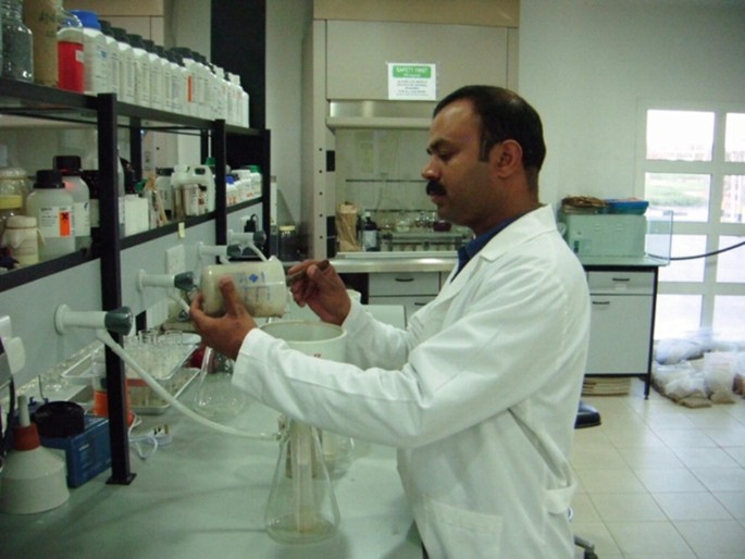

  

  Setup for collection of extract from saturated soil paste

• Continue filtration until the soil paste on the Buchner funnel begins to develop cracks

• If the filtrate is not clear (cloudy/turbid), it should be re-filtered through another wet filter paper to obtain a clear extract. Finally, transfer the clear filtrate into a 50 ml bottle

• Switch on the conductivity meter, immerse the electrode in the soil saturation extract and record the EC reading

• Remove the conductivity cell from the filtrate, rinse it thoroughly with DI water from a squirt bottle, and carefully dry the electrode with a tissue paper

• If accurate comparisons of ECe are to be made across a range of samples, the temperature of the extract must be measured and a correction factor (to 25 °C) utilized. The instruments available these days automatically correct the reading to 25 °C

• Check accuracy of the EC meter using a 0.01 N KCl solution, which should give a reading of 1.413 dS m⁻¹ at 25 °C

16.2 Modern Methods of Soil Salinity Measurement

16.2.1 Salinity Probe

An activity meter with a salinity probe is very convenient and gives instant apparent electrical conductivity (ECa) information, which is expressed in mS cm⁻¹ and g l⁻¹. There are many models of equipment available to measure in-situ salinity. One is the German-made PNT3000 COMBI + model; it is commonly used in agriculture, horticulture and on landscape sites for rapid salinity assessment and monitoring. It provides an extended EC measuring range from 0 to 20 mS cm⁻¹ and from 20 to 200 mS cm⁻¹. The unit includes a 250 mm long stainless steel electrode for direct soil salinity measurements; an EC-plastic probe with platinum plated ring sensors and a high quality aluminum carrying case. Its operation is convenient and simple; only one button makes the full operation possible. It is essential, however, to validate ECa values with ECe from same soil locations. In any case, the ECa must be correlated to ECe for use in assessing a crop’s salt tolerance. Recently Shahid (2013) has established correlations between ECe and ECa measured by EC probe in a large number of saline fields.

ECa (Salinity Probe) Versus EC of Extracts (Varying Soil:Water Ratios)

For many reasons, laboratory analysis of the soil saturation extract is still the most common technique for assessing soil salinity. Salinity of the saturation extract (ECe) is considered to be the ‘standard procedure’ because the amount of water that a soil holds at saturation (the saturation percentage) is related to several important soil parameters, including texture, surface area, clay content, and cation exchange capacity (CEC).

Low soil to water ratios, for example 1:1; 1:2.5; 1:5, make extraction easier, but show a poorer relation to field moisture condition than the saturated paste. The choice of equipment or procedure depends upon several factors, including size of the area being evaluated, the depth of soil to be assessed, the number and frequency of the measurements, the accuracy required, and the availability of resources. The standard method of salinity monitoring involves collecting soil samples from the root-zone over a given period of time followed by their analysis in the laboratory as a soil saturation extract.

As a part of International Center for Biosaline Agriculture (ICBA) salinity monitoring program, the soil team collected a large number of soil samples from experimental plots which had been irrigated with water of varying salinity, up to a maximum of seawater (Plate 1.5). These samples were air-dried and processed in order to collect water extracts from soil:water suspensions of 1:1, 1:2.5, and 1:5, as well as soil extracts made from a saturated soil paste. The field conductivity (ECa) in mS cm⁻¹ using the salinity probe (field scout) was also measured. A simple statistical test was used to calculate the correlation and correlation coefficient (R ²), and to derive factors from it in order to convert ECa (determined at several soil water contents by the use of the salinity probe) to ECe.

Plate 1.5

Salinity monitoring in a grass field using salinity probe. (Field scout PNT 3000 COMBI +)

The correlations are developed for a fine sand (Soil Survey Division Staff 2017) textural class at ICBA experimental station (Table 1.3). The conversion factor for ECe determinations derived from the apparent EC (ECa) measured by the field scout in saline fields (Shahid 2013) was found to be: ECe = ECa × 3.81.

Table 1.3 Correlations of ECa measured by using the field scout (EC probe) with EC of 1:1, 1:2.5 and 1:5 (soil:water suspensions) and ECe

16.2.2 Electromagnetic Induction (EMI)

Salinity assessment and management at the farm level must help farmers improve crop productivity. The conventional field sampling followed by laboratory analysis is a tedious, expensive and time consuming process. There are other modern methods which can be used quickly and effectively in field salinity mapping, e.g. electromagnetic induction (EMI) using the EM38. EM38 is the most commonly used instrument in agricultural surveys, and gives a rapid assessment of the soil’s apparent electrical conductivity (ECa), expressed in mS m⁻¹.

The EM38 has a transmitter coil and a receiving coil. The transmitter coil induces an electrical current into the soil and the receiving coil records the resultant electromagnetic field. The EM38 allows for a maximum of 150 cm or 75 cm depth of exploration in the vertical and horizontal dipole modes, respectively (Plate 1.6). EC mapping using EMI is one of the simplest and least expensive salinity measurement tools. Integration of GIS information with salinity data yields salinity maps which can help farmers interpret crop yield variations, and provide a better understanding of the subtle salinity differences across agricultural fields. These salinity maps may allow farmers to develop more precise management zones and ultimately obtain higher yields.

Plate 1.6

EC measurement with EM 38 in vertical mode (left: grassland) and horizontal mode (right: Atriplex field)

Technological advances such as EMI have, in the last 40 years, revolutionized soil salinity assessment. McNeill (1980) was among the first investigators to describe how the EMI method can be used in assessing soil salinity. He presented the theoretical basis for the use of EM ground conductivity meters to map lateral variation in subsurface electrical conductivity. The approach, and the instrumentation developed (GEONICS EM31, EM34-3, EM38), gained almost immediate acceptance as a replacement for the traditional use of the 4-electrode resistivity (galvanic) traversing techniques, especially when it was demonstrated that the two types of soil surveys produced very similar results (Cameron et al. 1981).

Accordingly, the spatial distribution of soil salinity on the individual field (Cameron et al. 1981), the agricultural farm (Norman et al. 1995a, b), as well as district (Vaughan et al. 1995) and the regional (Williams and Baker 1982) scales has been described. Baerends et al. (1990) used the EM38 for a detailed salinity survey in an experimental area of 37 ha. They measured electrical conductivity of the soil at more than 3600 locations, reporting significant difference between the salinity of barren, fallow and cropped fields. Thus, barren fields have a high salinity, fallow fields a moderate salinity, and the cropped fields showed the lowest salinity. Baerends et al. (1990) found good agreement between the EM38 survey and the results of the visual agronomic salinity survey, with EM38 survey yielding results with a better resolution. The EMI method is also more sensitive to salinity changes, and can be carried out at any time of the year.

The EM38 instrument has been mobilized (Rhoades 1992) by mounting it on the front wheels of a farm vehicle. The EM readings can be made with the sensor positioned at several different heights above the ground in both horizontal (EMH) and vertical (EMV) magnetic coil configurations. By this adjustment, each stop requires about 20–30 s, with multiple readings being needed to calculate ECa (and, in turn, salinity) within soil depths of 0–30, 30–60, 60–90, and 90–120 cm. The intensive data set of salinity by depth and location can also be used to assess the adequacy of past leaching/drainage practices (Rhoades 1992). For example, where salinity decreases with depth in the profile, the net flux of water (and salt) can be interpreted as being upward. This is reflective of inadequate leaching and/or poor drainage. Where salinity increases with depth in the soil profile, the net flux of water and salt can be inferred as being downward. This finding would be indicative of the adequacy of leaching/drainage. However, when salinity is low and relatively uniform with increasing depth, leaching is interpreted as excessive, probably contributing to waterlogging elsewhere, with a high salt loading of the receiving water supplies.

Rhoades and Ingvalson (1971) showed that soil salinity in the field could also be assessed with a conventional geo-electrical method. This method has been developed for the purposes of measuring the soil salinity of the entire root-zone (Nadler and Frenkel 1980; Rhoades and Oster 1986; Yadav et al. 1979). Elaborating the same technique, Rhoades and Van Schilfgaarde (1976) developed another electrical conductivity probe for measuring soil salinity distribution with increasing depth. With this probe, soil salinity is measured at specific depths in the root-zone. Thus, four electrode techniques can be successfully used for surveys of saline soils (Nadler 1981; Halvorson et al. 1977).

Williams and Baker (1982) first recognized the possibility of using EM meters for reconnaissance surveys of soil salinity variation. The high values of apparent electrical conductivity (ECa) measured by the EM meters were positively correlated with increased amounts of salts in the soil. The correlation led to empirical relationships (Rhoades et al. 1989; Cook et al. 1992; Acworth and Beasley 1998) that allow a prediction of soil salinity based on the measurement of the ECa. The correlation between salt content and the ECa is very high for zones of uniform soil material; though with zones showing different electrical conductivity, it is necessary to obtain separate values of ECa for each zone.

There is an electrical conductivity image method which provides an alternative approach. Here, the ECa function is sampled extensively in the vertical plane using a 4-electrode array. The method was described by Acworth and Griffiths (1985) and Griffiths and Baker (1993) but has not been widely used. There was difficulty in creating a starting model distribution of ECa values and extensive time consuming work was required in ‘forward modeling’ of the ECa data to achieve a match with the field data. Even so, the devices are used regularly for soil salinity surveys in different parts of the world (Boivin et al. 1988; Job et al. 1987; Williams and Hoey 1987). The main advantages of the EC image method are: i) measurements can be taken almost as fast as one can walk from one measurement location to another, and ii) the large volume of soil which is measured reduces the variability so that relatively fewer measurements yield a reliable estimate of the field’s mean salinity.

In one study (Nettleton et al. 1994), the EM induction approach has been extended to identification of sodium-affected soils. This approach shows great promise as a measure of both salinity and sodicity. However, such studies on sodic soils have not gained much attraction due to constraints in measuring accurate sodicity levels.

Factors Affecting EC Measurement of Soil by EM38

The conductance of electricity in soil takes place through the moisture filled pores that occur between individual soil particles. Therefore, the EC of soil is determined by the following soil properties (Doerge 1999).

Porosity

The greater soil porosity, the more easily electricity is conducted. Soil with high clay content has higher porosity than sandy soil. Compaction of moist soils normally increases soil EC.

Soil Water Content

Dry soil is much lower in electrical conductivity than moist soil.

Salinity Level

Increasing concentration of electrolytes (salts) in the soil water will dramatically increase soil EC.

Cation Exchange Capacity

Mineral soils which contain high levels of organic matter (humus) and/or 2:1 clay minerals, such as montmorillonite or vermiculite, have a much higher ability to retain positively charged ions (such as Ca²⁺, Mg²⁺, K⁺, Na⁺, NH₄ ⁺, or H⁺) than the soils lacking these constituents. The presence of these cations in moisture filled soil pores will enhance soil EC in the same way as salinity does.

Temperature

As temperature decreases toward the freezing point of water, soil EC decreases slightly. Below freezing point, soil pores become increasingly isolated from each other and overall soil EC declines rapidly.

16.2.3 Salinity Sensors and Data Logger

The most modern salinity data logging system is the Real Time Dynamic Automated Salinity Logging System (RTASLS). Here, ceramic salinity sensors are buried in the root-zone, each sensor being fitted with an external smart interface with a resolution of 16 Bits. This interface consists of an integrated microprocessor which contains all the required information to allow for autonomous operation of the sensor, including power requirements and logging interval. The smart interface is connected to a DataBus which leads to the Smart Data Logger which automatically identifies each of the salinity sensors and begins logging them at predetermined intervals. Instantaneous readings from sensors can be viewed in the field on the data logger’s display. Data can also be accessed in the field with a memory stick or remotely using a smart mobile phone. Due to technology advancements, there are diversified sensors available. Such a real time data logging system (Plate 1.7) has been installed in the grass plots at the experimental station of ICBA, Dubai (Shahid et al. 2008).

Plate 1.7

Real time salinity logging system at ICBA experimental station (Shahid et al. 2008) (a) Sensor placement in the root-zone, (b) Buried sensors connected to the Smart Interface, (c) Smart Interface connected to the DataBus, (d) Instantaneous salinity read on Data Logger

A useful feature of the salinity data logging system is that it does not require knowledge of electronics or computer programing. For custom configuring the Smart Data Logger or the salinity sensors, a simple menu system can be accessed through HyperTerminal. This provides complete control over each individual sensor’s setup. Data from the Smart Data Logger can be graphed using Excel.

16.2.3.1 System Installation and Operation – An Example

Salinity sensors are buried at 30 and 60 cm depths in a grass field (Distichlis spicata and Sporobolus virginicus) which is being irrigated with saline water of EC 10, 20 and 30 dS m⁻¹ (Plate 1.7). The dynamic changes of soil salinity within an irrigation cycle are showing the effect of salinity of the irrigation water on the salt concentration in the grass root-zone, and how the salt levels are constantly changing under irrigation (Fig. 1.6). The soil temperature can also give assistance with interpretation of soil-water movement as no soil moisture sensors were installed. Highlights of salinity monitoring for 25 days are presented in Fig. 1.6; note that days 15–19 are a period of rain.

Fig. 1.6

Soil salinity monitoring in a Distichlis spicata field at ICBA experimental station. Y-axis shows soil salinity fluctuations on different days. The experimental plots were irrigated with saline water of EC, dS m⁻¹: 10 (A, C), 20 (E, G) and 30 (I, K)

16.2.3.2 Soil Salinity Monitoring

The soil salinity data recorded in the Distichlis spicata grass field show that:

• After initial installation, it takes about 10 days for the sensors to come to equilibrium with the soil-water solution. This is especially apparent for the 30 dS m⁻¹ irrigation water treatment.

• Salinity levels for the 10 dS m⁻¹ irrigation water treatment are stable and typically 6–8 dS m⁻¹, with little change after rainfall.

• Salinity levels for the 20 dS m⁻¹ irrigation water treatment are 10 dS m⁻¹ at 30 cm and 14–16 dS m⁻¹ at 60 cm under the standard irrigation and management practice. Rainfall rapidly reduces the salinity level at both 30 cm and 60 cm soil depths. At 60 cm, the salinity level falls by 8–10 dS m⁻¹, e.g. from 16 to 6 dS m⁻¹.

• Salinity levels for the 30 dS m⁻¹ irrigation water treatment are above 20 dS m⁻¹ at 30 cm and 14–16 dS m⁻¹ at 60 cm under the standard irrigation and management practice. These salinity values are higher than those seen in the other treatments, reflecting the high salinity of the applied irrigation water.

• The sensitivity of the sensors to changing soil salinity levels is illustrated by both the diurnal fluctuation of salinity levels and the rapid changes that were observed (measured) after the rainfall. The diurnal data indicates a slight decline in soil salinity as the soil dries between 9:00 am and 4:00 pm, i.e. the time at which irrigation water is again applied.

16.3 Use of Remote Sensing (RS) and Geographical Information System (GIS) in Salinity Mapping and Monitoring

The RS and GIS have been used in many soil studies. Shahid (2013) has recently made efforts to compile this work in order to provide useful information to the potential users of these tools in soil salinity research. A comprehensive review is presented in the following section.

Salinity mapping can be accomplished by integrating RS and GIS techniques at both broad and small scales. The primary objective of reviewing publications dealing with these two techniques is to allow the prediction of sites vulnerable to the ‘salinity menace’. GIS is a computer application that involves the storage, analysis, retrieval, and display of data that are described in terms of their geographic location. The most familiar type of spatial data is a map – GIS is really a way of storing map information electronically. A GIS map has a number of advantages over old-style maps, a primary advantage being the fact that because the data are stored electronically, they can be analyzed readily by computer. In the case of soil salinity, scientists can use data on rainfall, topography and soil type (indeed, any spatial information that is available electronically can be used) to determine the factors which make soils highly susceptible to salinization with the aim of being able to predict other (similar) regions that may be at risk.

RS imagery is well suited to map the surface expression of salinity (Spies and Woodgate 2005). For example, a poor cover of vegetation could be an indication of salinity, especially when combined with information on depth of soil to groundwater. The goal of such an exercise is to assess and map soil salinity in order to better understand the problem, and then provide information on how to take necessary actions to prevent increases in salinization of new areas over time. And finally, we need to know how to best manage salinity for sustainable use of land resources.

Salinized and cropped areas can be identified and assigned a salinity index based on greenness and brightness – one that indicates leaf moisture of plants being influenced by salinity. Here, classical false-color composites of separated bands can be used, or a computer-assisted land-surface classification can be developed (Vincent et al. 1996). A brightness index detects brightness as representing a high level of salinity. Satellite images can help in assessing the extent of saline areas and can monitor changes in real time. Saline fields are often identified by the presence of spotty white patches of precipitated salts. Such precipitates usually occur in elevated or un-vegetated areas, where evaporation has left salt residues. Such salt crusts, which can be detected on satellite images, are, however, not reliable evidence of high salinity in the root-zone. Another limitation in salinity mapping with multispectral imagery is where saline soils support productive plant growth such as areas of biosaline agriculture. There, plant cover obscures direct sensing of the soil because salt tolerant plants cannot be differentiated from other ground cover, unless extensive on-site ground investigations are made to corroborate the information.

However, RS can provide useful information for large areas with differing water and salt balances and can identify parameters such as evapotranspiration, rainfall distribution, interception losses, and crop types and crop intensities that can be used as indirect measures of salinity and waterlogging as evidence in the absence of direct estimates (Ahmad 2002).

16.4 Global Use of Remote Sensing in Salinity Mapping and Monitoring

Salinity mapping and monitoring by using RS and GIS are common in many countries and such procedures have recently been used in Kuwait and Abu Dhabi Emirate as part of the National Soil Inventories (KISR 1999a,b; Shahid et al. 2002; EAD 2009). At regional and national levels (Sukchani and Yamamoto 2005), RS and GIS was used for waterlogging and salinity monitoring (Asif and Ahmed 1999). RS technology was used for soil salinity mapping in the Middle East (Hussein 2001) and salt-affected soils using RS and GIS (Maher 1990).

The Thematic Mapper^™ bands 5 and 7 are frequently used to detect soil salinity or drainage anomalies (Mulders and Epema 1986; Menenti et al. 1986; Zuluaga 1990; Vincent et al. 1996) and a broad scale monitoring of salinity using satellite remote sensing (Dutkiewics and Lewis 2008). Metternicht and Zinck (1997) have shown that Landsat TM (Thematic Mapper) and JERS-ISAR (Japan Earth Resources Satellite-Intelligent Synthetic Aperture Radar) data (visible and infrared regions) are the best ways to distinguish saline, alkaline, and non-saline soils. Landsat SMM (Solar Maximum Mission) and TM data for detailed mapping and monitoring of saline soils has been used in India for use as a reconnaissance soil map. Abdelfattah et al. (2009) developed a model that integrates remote sensing data with GIS techniques to assess, characterize, and map the state and behavior of soil salinity.

The coastal area of Abu Dhabi Emirate, where the issue of salinity is a major concern, has been used for a pilot study conducted in 2003. The development of a salinity model has been structured under four main phases: salinity detection using remote sensing data, site observations (on-site ground inspection), correlation and verification (a combination of a salinity map produced from visual interpretation of remotely sensed data and a salinity map produced from on-site observations), and model validation. Here, GIS was used to integrate the available data and information to design the model, and to create different maps. A geo-database was created and populated with data collected from observation points, melded together with laboratory analysis data. In this study, the correlation between the salinity maps developed from remote sensing data and on-site observations showed that 91.2% of the saline areas delineated using remote sensing data alone exhibit a good fit with saline areas delineated using on-site observations. Hence, the model can be adopted.

Remote sensing, thus, acquires information about the earth’s surface without actually being in contact with it. The fundamentals of remote sensing in soil salinity assessment and examples of such studies from the Middle East, Kuwait, Abu Dhabi Emirate and Australia have been described recently by Shahid et al. (2010). The combination of salinity maps taken over period of time and Digital Elevation Model (DEM) help to predict salinity risk in the area.

16.5 Geo-Statistics

Geo-statistics is used for mapping of land surface features from limited sample data. It is widely used in fields where ‘spatial’ data is studied. Geo-statistical estimation is a two-stage process. First step is studying the gathered data to establish the predictability of values from place-to-place within the study area. This results in a graph known as a semi-variogram, which models the difference between a value at one location and the value at another location according to the distance and direction between them. The second step is estimating values at those locations which have not been sampled. This process is known as ‘kriging’. The basic technique ‘ordinary kriging’ uses a weighted average of neighboring samples to estimate the ‘unknown’ value at a given location. Weights are optimized using the semi-variogram model, the locations of the samples, and all the relevant interrelationships between known and unknown values. The technique also provides a ‘standard error’ which may be used to calculate confidence levels. In mining, geo-statistics is extensively used in the field of mineral resource and reserve valuation, e.g. the estimation of grades and other parameters from a relatively small set of boreholes or other samples. Geo-statistics is now widely used in geological and geographical applications. However, the techniques are also used in such diverse fields as hydrology, groundwater, soil salinity mapping, and weather prediction. The application of geo-statistical techniques, such as ordinary- and co-kriging, have been applied to salinity survey data in an effort to represent more accurately the spatial distribution of soil salinity (Boivin et al. 1988; Vaughan et al. 1995).

In order to develop soil salinity maps, two approaches: Kriging and Inverse distance weighted (IDW) can be used, as explained below (Source: www.esri.com).

16.5.1 Kriging

Kriging is an advanced geo-statistical procedure that generates an estimated surface from a scattered set of points with z-values (elevation) (Fig. 1.7). Kriging assumes that the distance or direction between sample points reflects a spatial correlation that can be used to explain variation in the surface. The Kriging tool fits a mathematical function to a specified number of points, or to all points within a specified radius, in order to determine the output value for each location. As noted above, Kriging is a multistep process; it includes exploratory statistical analysis of the data, variogram modeling, creating the surface, and (optionally) exploring a variance surface. Kriging is most appropriate when you know there is a spatially correlated distance or directional bias in the data. It is often used in soil science and geology.

Fig. 1.7

Kriging method to generate salinity map

16.5.2 Inverse Distance Weighted (IDW) Interpolation

Inverse distance weighted interpolation determines cell values using a linearly weighted combination of a set of sample points (Fig. 1.8). The weight is a function of inverse distance. The surface being interpolated should be that of a location-dependent variable. This method assumes that the variable being mapped decreases in influence with distance from its sampled location.

Fig. 1.8

Inverse distance weighted (IDW) method to generate salinity map

16.6 Morphological Methods

Morphological details of salt minerals can be obtained at four levels, macro-, meso-, micro- and sub-microscopic levels, as described below:

16.6.1 Macromorphology

Macromorphology can be established during field investigation on a broad scale (Plate 1.8 upper left), and features of interest can be captured with digital camera (still or video). Such investigations quickly provide useful information about the area of interest.

16.6.2 Mesomorphology

Mesomorphological observations are made when the naked eye cannot resolve the details of the features of interest (Plate 1.8 upper right). The naked eye is then aided with hand lens or binocular microscope at lower magnifications. Such observations can be made in the field (hand lens) or in laboratory using binocular low magnification microscopes.

16.6.3 Micromorphology

Micromorphology

optical microscopy: When optical aid is needed for the naked eye to resolve details at higher magnifications, for example, in soil thin sections as studied with a polarizing microscope (Plate 1.8 bottom left); it is considered as an extension to field morphological studies. Soil thin sections are prepared by impregnating the saline soils with resin and hardened. After the resin has fully polymerized, the impregnated samples are cut into slices with diamond saw. The impregnated block is washed with petroleum spirit in an ultrasonic bath. One face of the impregnated soil block is then ground and polished successively with 6 and 3 μm diamond paste using Hyprez fluid as lubricant on polishing and lapping machine. The polished block is stuck to glass slide using resin and then ground to 25 μm thicknesses using lapping and polishing machine (Shahid 1988).

Micromorphology

submicroscopy: Is the resolution of details at the submicroscopic level (Plate 1.8 bottom right) using an electron microscope (scanning and transmission). For submicroscopic investigation, the base of the sample and the surface of the stub are painted with a silver colloid suspension by a brush and then sample is mounted onto the stub using normal araldite. The prepared mounted samples are either carbon coated under vacuum or coated with a layer of gold-palladium (20–30 nm thick) to prevent charge buildup on the specimen, and to hold the surface of the sample and a constant electric potential. The prepared samples are then studied using the scanning electron microscopy.

The above details can be obtained as required. The microscopy techniques can also be combined. For example, Bisdom (1980) coupled optical microscopy with submicroscopic methods and later with contact microradiography (Drees and Wilding 1983). The electron microscopes can be supplemented with a micro-chemical analyzer (Energy Dispersive X Ray Analyses – EDXRA, Wavelength Dispersive X Ray Analyses – WDXRA), thereby allowing in-situ micro-chemical analyses (non-destructive). To study salt crusts at the submicroscopic level, soil samples need coating with gold-palladium (an alloy), or carbon applied to salt crusts is needed to make the sample a conductor. The use of submicroscopic techniques has widely been used in salt minerals studies, such as in Turkey (Vergouwen 1981) and Pakistan (Shahid 1988; Shahid et al. 1990; Shahid et al. 1992; Shahid and Jenkins 1994; Shahid 2013) (Plate 1.8).

Plate 1.8

Salt features at different observations scales (cf. Shahid 1988; 2013). (a) Macroscopic features of soil salinity – naked eye observation (salt crust) (Width 20 meters), (b) Mesomorphological features – binocular observation of nahcolite (NaHCO3) mineral (Width 1100 μm), (c) Micromorphological feature – optical microscopic observation of thenardite (Na₂SO₄) mineral in thin section (Width 1000뭱μm), (d) Micromorphological feature – submicroscopic observation of lath shaped glauberite [(Na₂Ca (SO₄)₂] mineral – scanning electron microscopy (Width 64뭱μm)

References

Abdelfattah MA, Shahid SA, Othman YR (2009) Soil salinity mapping model developed using RS and GIS – a case study from Abu Dhabi, United Arab Emirates. Eur J Sci Res 26(3):342–351
Acworth RI, Beasley R (1998) Investigation of EM31 anomalies at Yarramanbah/Pump Station creek on the Liverpool Plains of New South Wales. WRL Research Report No 195. University of New South Wales, Sydney, Australia, 70 pp
Acworth RI, Griffiths DH (1985) Simple data processing of tripotential apparent resistivity measurements as an aid to the interpretation of subsurface structure. Geophys Prospect 33(6):861–867
Ahmad MD (2002) Estimation of net groundwater use in irrigated river basins using geo-information techniques: a case study in Rechna Doab, Pakistan. PhD Thesis, Wageningen University, Enschede, The Netherlands, 144 pp. http://edepot.wur.nl/121368
Akramkhanov A, Sommer R, Martius C, Hendrickx JMH, Vlek PLG (2008) Comparison and sensitivity of measurement techniques for spatial distribution of soil salinity. Irrig Drain Syst 22(1):115–126
Alavipanah SK, Zehtabian GR (2002) A database approach for soil salinity mapping and generalization from remote sensing data and geographic information system. FIG XXII International Congress, 19–26 April 2002, Washington DC, USA pp 1–8
Al-Moustafa WA, Al-Omran AM (1990) Reliability of 1:1, 1:2, and 1:5 weight extracts for expressing salinity in light-textured soils of Saudi Arabia. J King Saud Univ Agric Sci 2(2):321–329
Asif S, Ahmed MD (1999) Using state-of-the-art RS and GIS for monitoring waterlogging and salinity. International Water Management Institute, Lahore, Pakistan, 16 pp
Baerends B, Raza ZI, Sadiq M, Chaudhry MA, Hendrickx JMH (1990) Soil salinity survey with an electromagnetic induction method. Proceedings of the Indo-Pak workshop on soil salinity and water management, 10–14 February 1990, Islamabad, Pakistan, vol 1. pp 201–219
Bisdom EBA (1980) A review of the application of submicroscopy techniques in soil micromorphology. I. Transmission electron microscopy (TEM) and scanning electron microscopy (SEM). In: Bisdom EBA (ed) Submicroscopy of soils and weathered rocks. Pudoc, Wageningen, pp 67–116
Boivin P, Hachicha M, Job JO, Loyer JY (1988) Une méthode de cartographie de la salinité des sols: conductivité électromagnétique et interpolation par krigeage. Sci du sol 27:69–72
Cameron DR, De Jong E, Read DWL, Oosterveld M (1981) Mapping salinity using resistivity and electromagnetic inductive techniques. Can J Soil Sci 61:67–78
Cook PG, Walker GR, Buselli G, Potts I, Dodds AR (1992) The application of electromagnetic techniques to groundwater recharge investigations. J Hydrol 130:201–229
Doerge T (1999) Soil electrical conductivity mapping. Crop Insights 9(19):1–4
Drees LR, Wilding LP (1983) Microradiography as a submicroscopic tool. Geoderma 30:65–76
Dutkiewics A, Lewis M (2008) Broadscale monitoring of salinity using satellite remote sensing: where to from here? 2nd International Salinity Forum Adelaide, Australia, 6 pp
EAD (2009) Soil survey of Abu Dhabi Emirate. Environment Agency Abu Dhabi. 5 Volumes
EAD (2012) Soil survey of Northern Emirates. Environment Agency Abu Dhabi. 2 Volumes
FAO-UNESCO (1974) Soil map of the world. 1:5,000,000, vol 1–10. UNESCO, Paris
Franklin WT, Follett RH (1985) Crop tolerance to soil salinity. No. 505. Service in action: Colorado State University Extension Service
Griffiths DH, Baker RD (1993) Two-dimensional resistivity imaging and modeling in areas of complex geology. J Appl Geophys 29:211–226
Halvorson AD, Rhoades JD, Reule CA (1977) Soil salinity – four-electrode conductivity relationships for soils of the northern great plains. Soil Sci Soc Am J 41(5):966–971
Hogg TJ, Henry JL (1984) Comparison of 1:1 and 1:2 suspensions with the saturation extract in estimating salinity in Saskatchewan soils. Can J Soil Sci 64(4):699–704
Hussein H (2001) Development of environmental GIS database and its application to desertification study in Middle East. A Remote sensing and GIS application. PhD Thesis Graduate School of Science and Technology, Chiba University Japan, 155 pp
Job JO, Loyer JY, Ailoul M (1987) Utilisation de la conductivite electromagnetique pour la mesure directe de la salinite des sols. Cah ORSTOM, ser Pedol 23(2):123–131
KISR (1999a) Soil survey for the state of Kuwait – Volume II: Reconnaissance survey. AACM International, Adelaide
KISR (1999b) Soil survey for the state of Kuwait – Volume IV: Semi-detailed survey. AACM International, Adelaide
Landon JR (ed) (1984) Booker tropical soil manual, Paperback edn. Routledge Taylor & Francis Group, New York/London, 474 pp
Maher MAA (1990) The use of remote sensing techniques in combination with a geographic information system for soil studies with emphasis on quantification of salinity and alkalinity in the northern part of the Nile delta. MSc thesis Enschede Netherlands, ITC
McNeill JD (1980) Electromagnetic terrain conductivity measurements at low induction numbers. Geonics Limited Technical Notes TN-6, Geonics Ltd, Mississauga, Ontario, Canada 15 pp
Menenti M, Lorkeers A, Vissers M (1986) An application of thematic mapper data in Tunisia. ITC J 1:35–42
Metternicht GB, Zinck JA (1997) Spatial discrimination of salt- and sodium-affected soil surfaces. Int J Remote Sens 18(12):2571–2586
Mulders MA, Epema GF (1986) The thematic mapper: a new tool for soil mapping in arid areas. ITC J 1:24–29
Nadler A (1981) Field application of the four-electrode technique for determining soil solution conductivity. Soil Sci Soc Am J 45:30–34
Nadler A, Frenkel H (1980) Determination of soil solution electrical conductivity from bulk soil electrical conductivity measurements by the four-electrode method. Soil Sci Soc Am J 44:1216–1221
Nettleton WD, Bushue L, Doolittle JA, Endres TJ, Indorante SJ (1994) Sodium-affected soil identification in South-Central Illinois by electromagnetic induction. Soil Sci Soc Am J 58:1190–1193
Norman C, Challis P, Oliver H, Robinson J, Gillespie K, Rankin C, Tonkins S, Heath J (1995a) Whole farm soil salinity surveys in the Kerang region. Institute of Sustainable Irrigated Agriculture (ISIA), Tatura, Report 1993–1995, p 162
Norman C, Heath J, Turnour R, MacDonald P (1995b) On-farm salinity monitoring and investigations. Institute of Sustainable Irrigated Agriculture (ISIA), Tatura, Report 1993–1995, p 164
Rhoades JD (1992) Instrumental field methods of salinity appraisal. In: Topp GC, Reynolds WD, Green RE (eds) Advances in measurements of soil physical properties: Bringing theory into practice. SSSA Special Publication 30/ASA/CSSA/SSSA, Madison, pp 231–248
Rhoades JD, Ingvalson RD (1971) Determining salinity in field soils with soil resistance measurements. Soil Sci Soc Am Proc 35(1):54–60
Rhoades JD, Oster JD (1986) Solute content. In: Klute A (ed) Methods of soil analysis, part 1, 2nd edn. Agronomy 9:985–1006
Rhoades JD, van Schilfgaarde J (1976) An electrical conductivity probe for determining soil salinity. Soil Sci Soc Am Proc 40:647–655
Rhoades JD, Manteghi NA, Shouse PJ, Alves WJ (1989) Soil electrical conductivity and soil salinity: New formulations and calibrations. Soil Sci Soc Am J 53(2):433–439
Shahid SA (1988) Studies on the micromorphology of salt-affected soils of Pakistan. PhD Thesis, University College of North Wales, Bangor, UK. 2 Volumes
Shahid SA (1993) Effect of saline-sodic waters on the hydraulic conductivity and soil structure of the simulated experimental soil columns. Proceedings of the International Symposium on Environmental Assessment and Management of Irrigation and Drainage Projects for Sustained Agricultural Growth, 11–13 April 1993, Lahore, Pakistan, vol 2. pp 125–138
Shahid SA (2013) Developments in salinity assessment, modeling, mapping, and monitoring from regional to submicroscopic scales. In: Shahid SA, Abdelfattah MA, Taha FK (eds) Developments in soil salinity assessment and reclamation – innovative thinking and use of marginal soil and water resources in irrigated agriculture. Springer, Dordrecht/Heidelberg/New York/London, pp 3–43
Shahid SA, Jenkins DA (1991a) Effect of successive waters of different quality on hydraulic conductivity of a soil. J Drain Reclam 3(2):9–13
Shahid SA, Jenkins DA (1991b) Mechanisms of hydraulic conductivity reduction in the Khurrianwala soil series. Pak J Agric Sci 28(4):369–373
Shahid SA, Jenkins DA (1992a) Development of a simulation system for quick screening of soils against salinity and sodicity. In: Feyen J, Mwendera E, Badji M (eds) Advances in planning, design and management of irrigation systems as related to sustainable land use: proceedings of an international conference, 14–17 September 1992, vol 2. Center for Irrigation Engineering of the Katholieke Universiteit Leuven, Leuven, pp 607–614
Shahid SA, Jenkins DA (1992b) Micromorphology of surface and subsurface sealing and crusting in the soils of Pakistan. In: Vlotman WF (ed) Subsurface drainage on problematic irrigated soils: sustainability and cost effectiveness. Proceedings of the 5th international drainage workshop, 8–15 February 1992, Lahore, Pakistan, vol 2. pp 177–189
Shahid SA, Jenkins DA (1992c) Utilization of simulation system for quick screening of soils against salinity and sodicity. In: Feyen J, Mwendera E, Badji M (eds) Advances in planning design and management of irrigation systems as related to sustainable land use: proceedings of an international conference, 14–17 September 1992, vol 2. Center for Irrigation Engineering of the Katholieke Universiteit Leuven, Leuven, pp 615–626
Shahid SA, Jenkins DA (1994) Mineralogy and micromorphology of salt crusts from the Punjab, Pakistan. In: Ringrose-Voase AJ, Hymphreys GS (eds) Soil micromorphology: studies in management and genesis, developments in soil science 22, Proceedings of the IX international working meeting on soil micromorphology, July 1992, Townsville, Australia, Elsevier Amsterdam London New York Tokyo pp 799–810
Shahid SA, Rahman KR (2011) Soil salinity development, classification, assessment and management in irrigated agriculture. In: Passarakli M (ed) Handbook of plant and crop stress. CRC Press/Taylor & Francis Group, Boca Raton, pp 23–39
Shahid SA, Qureshi RH, Jenkins DA (1990) Salt-minerals in the saline-sodic soils of Pakistan. Proceedings of the Indo-Pak workshop on soil salinity and water management, 10–14 February 1990, Islamabad, Pakistan, vol 1. pp 175–191
Shahid SA, Jenkins DA, Hussain T (1992) Halite morphologies and genesis in the soil environment of Pakistan. Proceedings of the International Symposium on Strategies for Utilizing Salt-affected Lands, 17–25 February 1992, Bangkok, Thailand pp 59–73
Shahid SA, Abo-Rezq H, Omar SAS (2002) Mapping soil salinity through a reconnaissance soil survey of Kuwait and geographic information system. Annual Research Report, Kuwait Institute for Scientific Research, Kuwait, KSR 6682 pp 56–59
Shahid SA, Dakheel AH, Mufti KA, Shabbir G (2008) Automated in-situ salinity logging in irrigated agriculture. Eur J Sci Res 26(2):288–297
Shahid SA, Abdefattah MA, Omar SAS, Harahsheh H, Othman Y, Mahmoudi H (2010) Mapping and monitoring of soil salinization – remote sensing, GIS, modeling, electromagnetic induction and conventional methods – case studies. In: Ahmad M, Al-Rawahy SA (eds) Proceedings of the international conference on soil salinization and groundwater salinization in arid regions, vol 1. Sultan Qaboos University, Muscat, pp 59–97
Shahid SA, Abdelfattah MA, Mahmoudi H (2013) Innovations in soil chemical analyses: New ECs and total salts relationship for Abu Dhabi emirate soils. In: Shahid SA, Taha FK, Abdelfattah MA (eds) Developments in soil classification, land use planning and policy implications – innovative thinking of soil inventory for land use planning and Management of Land Resources. Springer, Dordrecht, pp 799–812
Shirokova YI, Forkutsa I, Sharafutdinova N (2000) Use of electrical conductivity instead of soluble salts for soil salinity monitoring in Central Asia. Irrig Drain Syst 14(3):199–205
Soil Survey Division Staff (2017) Soil survey manual. USDA-NRCS Agriculture Handbook No 18, US Government Printing Office, Washington DC, USA, 603 pp
Sonmez S, Bukuktas D, Okturen F, Citak S (2008) Assessment of different soil water ratios (1:1, 1:2.5, 1:5) in soil salinity studies. Geoderma 144(1–2):361–369
Spies B, Woodgate P (2005) Salinity mapping methods in the Australian context. Technical Report, Department of the Environment and Heritage; and Agriculture, Fisheries and Forestry, Land and Water Australia, Canberra, Australia, 234 pp
Sukchani S, Yamamoto Y (2005) Classification of salt-affected areas using remote sensing. Soil survey and classification division. Department of Land Development, Ministry of Agriculture and Cooperative, Bangkok, Thailand and Japan International Research Center Agricultural Sciences, Tsukuba, Ibaraki, Japan, 7 pp
Tanji KK (1990) Nature and extent of agricultural salinity. In: Tanji KK (ed) Agricultural salinity assessment and management, ASCE manuals and reports on engineering practice No 71. ASCE, New York, USA, pp 1–17
Triantafilis J, Laslett GM, McBratney AB (2000) Calibrating an electromagnetic induction instrument to measure salinity in soil under irrigated cotton. Soil Sci Soc Am J 64(3):1009–1017
USSL Staff (1954) Diagnosis and improvement of saline and alkali soils. USDA Handbook No 60 Washington DC, USA, 160 pp
Vaughan PJ, Lesch SM, Crown DL, Cone DG (1995) Water content effect on soil salinity prediction. A geostatistical study using co-kriging. Soil Sci Soc Am J 59(4):1146–1156
Vergouwen L (1981) Scanning electron microscopy applied on saline soils from the Konya basin in Turkey and from Kenya. In: Bisdom EBA (ed) Submicroscopy of soil and weathered rocks. Center for Agricultural Publishing and Documentation, Wageningen, pp 237–248
Vincent B, Vidal A, Tabbet D, Baqri A, Kapur M (1996) Use of satellite remote sensing for the assessment of waterlogging or salinity as an indication of the performance of drained systems. In: Vincent B (ed) Evaluation of performance of subsurface drainage systems. Proceedings of the 16th congress on irrigation and drainage, Cairo, ICID New Delhi, India pp 203–216
Williams BG, Baker GC (1982) An electromagnetic induction technique for reconnaissance survey of salinity hazards. Aust J Soil Res 20(2):107–118
Williams BG, Hoey D (1987) The use of electromagnetic induction to detect the spatial variability of the salt and clay contents of soils. Aust J Soil Res 25(1):21–27
Yadav BR, Rao NH, Paliwal KV, Sharma PBS (1979) Comparison of different methods for measuring soil salinity under field conditions. Soil Sci 127(26):335–339
Zheng H, Schroder JL, Pittman JJ, Wang JJ, Payton ME (2005) Soil salinity using saturated paste and 1:1 soil to water extracts. Soil Sci Soc Am J 69(4):1146–1151
Zuluaga JM (1990) Remote sensing applications in irrigation management in Mendoza, Argentina. In: Menenti M (ed) Remote sensing in evaluation and management of irrigation. Instituto Nacional de Ciencia y Tecnic, Mendoza, pp 37–58
Author information
Authors and Affiliations
Corresponding author
Rights and permissions
The opinions expressed in this chapter are those of the author(s) and do not necessarily reflect the views of the IAEA, its Board of Directors, or the countries they represent
Open Access This chapter is licensed under the terms of the Creative Commons Attribution 3.0 IGO License (https://creativecommons.org/licenses/by/3.0/igo/), which permits use, sharing, adaptation, distribution and reproduction in any medium or format, as long as you give appropriate credit to the IAEA, provide a link to the Creative Commons licence and indicate if changes were made.
The use of the IAEA's name, and the use of the IAEA's logo, shall be subject to a separate written licence agreement between the IAEA and the user and is not authorized as part of this CC-IGO licence. Note that the link provided above includes additional terms and conditions of the licence.
The images or other third party material in this chapter are included in the chapter's Creative Commons licence, unless indicated otherwise in a credit line to the material. If material is not included in the chapter's Creative Commons licence and your intended use is not permitted by statutory regulation or exceeds the permitted use, you will need to obtain permission directly from the copyright holder.
Copyright information
© 2018 International Atomic Energy Agency
About this chapter
Cite this chapter
Shahid, S.A., Zaman, M., Heng, L. (2018). Introduction to Soil Salinity, Sodicity and Diagnostics Techniques. In: Guideline for Salinity Assessment, Mitigation and Adaptation Using Nuclear and Related Techniques . Springer, Cham. https://doi.org/10.1007/978-3-319-96190-3_1
Download citation
DOI: https://doi.org/10.1007/978-3-319-96190-3_1
Published:
Publisher Name: Springer, Cham
Print ISBN: 978-3-319-96189-7
Online ISBN: 978-3-319-96190-3
eBook Packages: Earth and Environmental ScienceEarth and Environmental Science (R0)