
Abstract
Collision resistant hash functions are functions that shrink their input, but for which it is computationally infeasible to find a collision, namely two strings that hash to the same value (although collisions are abundant).
In this work we study multi-collision resistant hash functions (\(\mathsf {MCRH}\)) a natural relaxation of collision resistant hash functions in which it is difficult to find a t-way collision (i.e., t strings that hash to the same value) although finding \((t-1)\)-way collisions could be easy. We show the following:
-
The existence of \(\mathsf {MCRH}\) follows from the average case hardness of a variant of the Entropy Approximation problem. The goal in this problem (Goldreich, Sahai and Vadhan, CRYPTO ’99) is to distinguish circuits whose output distribution has high entropy from those having low entropy.
-
\(\mathsf {MCRH}\) imply the existence of constant-round statistically hiding (and computationally binding) commitment schemes. As a corollary, using a result of Haitner et al. (SICOMP, 2015), we obtain a blackbox separation of \(\mathsf {MCRH}\) from any one-way permutation.
The full version [BDRV17] is available at https://eprint.iacr.org/2017/489.
You have full access to this open access chapter, Download conference paper PDF
1 Introduction
Hash functions are efficiently computable functions that shrink their input and mimic ‘random functions’ in various aspects. They are prevalent in cryptography, both in theory and in practice. A central goal in the study of the foundations of cryptography has been to distill the precise, and minimal, security requirements necessary from hash functions for different applications.
One widely studied notion of hashing is that of collision resistant hash functions (\(\mathsf {CRH}\)). Namely, hash functions for which it is computationally infeasible to find two strings that hash to the same value, even when such collisions are abundant. \(\mathsf {CRH}\) have been extremely fruitful and have notable applications in cryptography such as digital signaturesFootnote 1 [GMR88], efficient argument systems for \(\texttt {NP}\) [Kil92, Mic00] and (constant-round) statistically hiding commitment schemes [NY89, DPP93, HM96].
In this work we study a natural relaxation of collision resistance. Specifically, we consider hash functions for which it is infeasible to find a t-way collision: i.e., t strings that all have the same hash value. Here t is a parameter, where the standard notion of collision resistance corresponds to the special case of \(t=2\). We refer to such functions as multi-collision resistant hash functions \((\mathsf {MCRH})\) and emphasize that, for \(t>2\), it is a weaker requirement than that of standard collision resistance.
The property of multi-collision resistance was considered first by Merkle [Mer89] in analyzing a hash function construction based on DES. The notion has also been considered in the context of identification schemes [GS94], micro-payments [RS96], and signature schemes [BPVY00]. Joux [Jou04] showed that for iterated hash functions, finding a large number of collisions is no harder than finding pairs of highly structured colliding inputs (namely, collisions that share the same prefix). We emphasize that Joux’s multi-collision finding attack only applies to certain types of hash functions (e.g., iterated hash functions, or tree hashing) and requires a strong break of collision resistance. In general, it seems that \(\mathsf {MCRH}\) is a weaker property than \(\mathsf {CRH}\).
As in the case of \(\mathsf {CRH}\), to obtain a meaningful definition, we must consider keyed functions (since for non keyed functions there are trivial non-uniform attacks). Thus, we define \(\mathsf {MCRH}\) as follows (here and throughout this work, we use \(n\) to denote the security parameter.)
Definition 1.1
((s, t)-\(\mathsf {MCRH}\)). Let \(s = s(n) \in \mathbb {N}\) and \(t = t(n) \in \mathbb {N}\) be functions computable in time  . An (s, t)-Multi-Collision Resistant Hash Function Family ((s, t)-\(\mathsf {MCRH}\)) consists of a probabilistic polynomial-time algorithm
  that on input \(1^n\) outputs a circuit h such that:
-
s-Shrinkage: The circuit
 maps inputs of length \(n\) to outputs of length \(n-s\).
 -
t-Collision Resistance: For every polynomial size family of circuits
 ,
, 
 maps inputs of length
  ,
, 
Note that the standard notion of \(\mathsf {CRH}\) simply corresponds to (1, 2)-\(\mathsf {MCRH}\) (which is easily shown to be equivalent to (s, 2)-\(\mathsf {CRH}\) for any \(s=n- \omega (\log {n})\)). We also remark that Definition 1.1 gives a non-uniform security guarantee, which is natural, especially in the context of collision resistance. Note though that all of our results are obtained by uniform reductions.
Remark 1.2
(Shrinkage vs. Collision Resistance). Observe that (s, t)-\(\mathsf {MCRH}\) are meaningful only when \(s \ge \log {t}\), as otherwise t-way collisions might not even exist (e.g., consider a function mapping inputs of length n to outputs of length \(n-\log (t-1)\) in which each range element has exactly \(t-1\) preimages).
Moreover, we note that in contrast to standard \(\mathsf {CRH}\), it is unclear whether the shrinkage factor s can be trivially improved (e.g., by composition) while preserving the value of t. Specifically, constructions such as Tree Hashing (aka Merkle Tree) inherently rely on the fact that it is computationally infeasible to find any collision. It is possible to get some trade-offs between the number of collisions and shrinkage. For example, given an \( (s=2, t = 4) \)-\( \mathsf {MCRH}\), we can compose it with itself to get an \( (s=4, t = 10) \)-\( \mathsf {MCRH}\). But it is not a priori clear whether there exist transformations that increase the shrinkage s while not increasing t. We remark that a partial affirmative answer to this question was recently given in an independent and concurrent work by Bitansky et al. [BPK17], as long as the hash function is substantially shrinking (see additional details in Sect. 1.2).
Thus, we include both the parameters s and t in the definition of \(\mathsf {MCRH}\), whereas in standard \(\mathsf {CRH}\) the parameter t is fixed to 2, and the parameter s can be given implicitly (since the shrinkage can be trivially improved by composition).
Remark 1.3
(Scaling of Shrinkage vs. Collisions). The shrinkage s is measured in bits, whereas the number of collisions t is just a number. A different definitional choice could have been to put s and t on the same “scale” (e.g., measure the logarithm of the number of collisions) so to make them more easily comparable. However, we refrain from doing so since we find the current (different) scaling of s and t to be more natural.
Remark 1.4
(Public-coin \(\mathsf {MCRH}\)). One can also consider the stronger public-coin variant of \(\mathsf {MCRH}\), in which it should be hard to find collisions given not only the description of the hash function, but also the coins that generated the description.
Hsiao and Reyzin [HR04] observed that for some applications of standard collision resistance, it is vital to use the public-key variant (i.e., security can be broken in case the hash function is not public-coin). The distinction is similarly important for \(\mathsf {MCRH}\) and one should take care of which notion is used depending on the application. Below, when we say \(\mathsf {MCRH}\), we refer to the private-coin variant (as per Definition 1.1).
1.1 Our Results
The focus of this work is providing a systematic study of \(\mathsf {MCRH}\). We consider both the question of constructing \(\mathsf {MCRH}\) and what applications can we derive from them.
1.1.1 Constructions of \(\mathsf {MCRH}\)
Since any \(\mathsf {CRH}\) is in particular also an \(\mathsf {MCRH}\), candidate constructions are abundant (based on a variety of concrete computational assumptions). The actual question that we ask, which has a more foundational flavor, is whether we can construct \(\mathsf {MCRH}\) from assumptions that are not known to imply \(\mathsf {CRH}\).
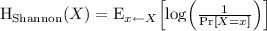
Our first main result is that the existence of \(\mathsf {MCRH}\) follows from the average-case hardness of a variant of the Entropy Approximation problem studied by Goldreich, Sahai and Vadhan [GSV99]. Entropy Approximation, denoted \(\mathsf {EA}_{}^{}\), is a promise problem, where YES inputs are circuits whose output distribution (i.e., the distribution obtained by feeding random inputs to the circuit) has entropy at least k, whereas NO inputs are circuits whose output distribution has entropy at most \(k-1\) (where k is a parameter that is unimportant for the current discussion). Here by entropy we specifically refer to Shannon entropy.Footnote 2 Goldreich et al. showed that \(\mathsf {EA}_{}^{}\) is complete for the class of (promise) problems that have non-interactive statistical zero-knowledge proofs ( ).
).
In this work we consider a variant of \(\mathsf {EA}_{}^{}\), first studied by Dvir et al. [DGRV11], that uses different notions of entropy. Specifically, consider the promise problem \(\mathsf {EA}_{\min ,\max }^{}\), where the goal now is to distinguish between circuits whose output distribution has min-entropyFootnote 3 at least k from those with max-entropy at most \(k-1\). It is easy to verify that \(\mathsf {EA}_{\min ,\max }^{}\) is an easier problem than \(\mathsf {EA}_{}^{}\).
Theorem 1.1
(Informal, see Theorem 3.6). If \(\mathsf {EA}_{\min ,\max }^{}\) is average-case hard, then there exist (s, t)-\(\mathsf {MCRH}\), where \( s = \sqrt{n} \) and \( t = 6n^2 \).
(Note that in the \(\mathsf {MCRH}\) that we construct there exist \(2^{\sqrt{n}}\)-way collisions, but it is computationally hard to find even a \(6n^2\)-way collision.)
In contrast to the original entropy approximation problem, we do not know whether \(\mathsf {EA}_{\min ,\max }^{}\) is complete for  . Thus, establishing the existence of \(\mathsf {MCRH}\) based solely on the average-case hardness of
  (or
(or  ) remains open. Indeed such a result could potentially be an interesting extension of Ostrovsky’s [Ost91] proof that average-case hardness of
  implies the existence of one-way functions.
Instantiations. Dvir et al. [DGRV11], showed that the average-case hardness of \(\mathsf {EA}_{\min ,\max }^{}\) is implied by either the quadratic residuocity (\(\mathsf {QR}\)) or decisional Diffie Hellman (\(\mathsf {DDH}\)) assumptions.Footnote 4 It is not too hard to see that above extends to any encryption scheme (or even commitment scheme) in which ciphertexts can be perfectly re-randomized.Footnote 5
The hardness of \(\mathsf {EA}_{\min ,\max }^{}\) can also be shown to follow from the average-case hardness of the Shortest Vector Problem or the Closest Vector Problem with approximation factor roughly \(\sqrt{n}\).Footnote 6 To the best of our knowledge the existence of \(\mathsf {CRH}\) is not known based on such small approximation factors (even assuming average-case hardness).
We remark that a similar argument establishes the hardness of \(\mathsf {EA}_{\min ,\max }^{}\) based on the plausible assumption that graph isomorphism is average-case hard.Footnote 7
1.1.2 Applications of \(\mathsf {MCRH}\)
The main application that we derive from \(\mathsf {MCRH}\) is a constant-round statistically hiding commitment scheme.
Theorem 1.2
(Informally stated, see Theorem 4.4). Assume that there exists a \((\log (t),t)\)-\(\mathsf {MCRH}\). Then, there exists a 3-round statistically-hiding and computationally-binding commitment scheme.
We note that Theorem 1.2 is optimal in the sense of holding for \(\mathsf {MCRH}\) that are minimally shrinking. Indeed, as noted in Remark 1.2, (s, t)-\(\mathsf {MCRH}\) with \(s\le \log (t-1)\) exist trivially and unconditionally.
It is also worthwhile to point out that by a result of Haitner et al. [HNO+09], statistically-hiding commitment schemes can be based on the existence of any one-way function. However, the commitment scheme of [HNO+09] uses a polynomial number of rounds of interaction and the main point in Theorem 1.2 is that we obtain such a commitment scheme with only a constant number of rounds.
Moreover, by a result of [HHRS15], any fully black-box construction of a statistically hiding commitment scheme from one-way functions (or even one-way permutations) must use a polynomial number of rounds. Loosely speaking, a construction is “fully black-box” [RTV04] if (1) the construction only requires an input-output access to the underlying primitive and (2) the security proof also relies on the adversary in a black-box way. Most constructions in cryptography are fully black-box. Since our proof of Theorem 1.2 is via a fully black-box construction, we obtain the following immediate corollary:
Corollary 1.3
(Informally stated). There does not exist a fully blackbox construction of \(\mathsf {MCRH}\) from one-way permutations.
Corollary 1.3 can be viewed as an extension of Simon’s [Sim98] blackbox separation of \(\mathsf {CRH}\) from one-way permutations. Due to space limitations, the formal statement and proof of Corollary 1.3 is deferred to the full version of this paper [BDRV17].
1.2 Related Works
Generic Constructions of \(\mathsf {CRH}\). Peikert and Waters [PW11] construct \( \mathsf {CRH}\) from lossy trapdoor functions. Their construction can be viewed as a construction of \( \mathsf {CRH}\) from \( \mathsf {EA}_{\min ,\max }^{} \) with a huge gap. (Specifically, the lossy trapdoor function h is either injective (i.e., \( {{\mathrm{H}}}_{\min }(h) \ge n\)) or very shrinking (i.e., \( {{\mathrm{H}}}_{\max }(h) < 0.5n\)).Footnote 8 One possible approach to constructing \( \mathsf {CRH}\) from lossy functions with small ‘lossiness’ (\( {{\mathrm{H}}}_{\max }(h)/{{\mathrm{H}}}_{\min }(h) \)) is to first amplify the lossiness and then apply the [PW11] construction. Pietrzak et al. [PRS12] rule out this approach by showing that it is impossible to improve the ‘lossiness’ in a black-box way.Footnote 9 We show that even with distributions where the gap is tiny, we can achieve weaker yet very meaningful notions of collision-resistance.
Applebaum and Raykov [AR16] construct \(\mathsf {CRH}\) from any average-case hard language with a Perfect Randomized Encoding in which the encoding algorithm is one-to-one as a function of the randomness. Perfect Randomized Encodings are a way to encode the computation of a function f on input x such that information-theoretically, the only information revealed about x is the value f(x). The class of languages with such randomized encodings \( \mathsf {PRE} \) is contained in \( \mathsf {PZK} \). Their assumption of an average-case hard language with a perfect randomized encoding implies \( \mathsf {EA}_{\min ,\max }^{} \) as well.
Constant-Round Statistically Hiding Commitments from  Hardness. The work of Ong and Vadhan [OV08] yields constant-round statistically-hiding commitment schemes from average-case hardness of
  .Footnote 10 Our construction of statistically-hiding commitments via \( \mathsf {MCRH}\) is arguably simpler, although it relies on a stronger assumption (\( \mathsf {EA}_{\min ,\max }^{} \)) instead of average-case hardness of
  .
.
Distributional \(\mathsf {CRH}\). A different weakening of collision resistance was considered by Dubrov and Ishai [DI06]. Their notion, called “distributional collision-resistant” in which it may be feasible to find some specific collision, but it is hard to sample a random collision pair. That is, given the hash function h, no efficient algorithm can sample a pair \((z_1,z_2)\) such that \(z_1\) is uniform and \(z_2\) is uniform in the set \(\{ z : h(z)=h(z_1)\}\). The notions of \(\mathsf {MCRH}\) and distributional \(\mathsf {CRH}\) are incomparable and whether one can be constructed from the other is open.
Min-Max Entropy Approximation. The main result of the work of Dvir et al. [DGRV11] (that was mentioned above) was showing that the problem \(\mathsf {EA}_{}^{}\) for degree-3 polynomial mappings (i.e., where the entropies are measured by Shannon entropy) is complete for  , a sub-class of
  in which the verifier and the simulator run in logarithmic space. They also construct algorithms to approximate different notions of entropy in certain restricted settings (but their algorithms do not violate the assumption that \(\mathsf {EA}_{\min ,\max }^{}\) is average-case hard).
1.2.1 Independent Works
\(\mathsf {MCRH}\) have been recently considered in an independent work by Komargodski et al. [KNY17b] (which was posted online roughly four months prior to the first public posting of our work). Komargodski et al. study the problem, arising from Ramsey theory, of finding either a clique or an independent set (of roughly logarithmic size) in a graph, when such objects are guaranteed to exist. As one of their results, [KNY17b] relate a variant of the foregoing Ramsey problem (for bipartite graphs) to the existence of \(\mathsf {MCRH}\). We emphasize that the focus of [KNY17b] is in studying computational problems arising from Ramsey theory, rather than \(\mathsf {MCRH}\) directly.
Beyond the work of [KNY17b], there are two other concurrent works that specifically study \(\mathsf {MCRH}\) [BPK17, KNY17a] (and were posted online simultaneously to our work). The main result of [KNY17a] is that the existence of \(\mathsf {MCRH}\) (with suitable parameters) implies the existence of efficient argument-systems for \(\texttt {NP}\), \(\acute{a}\) la Kilian’s protocol [Kil92]. Komargodski et al. [KNY17a] also prove that \(\mathsf {MCRH}\) imply constant-round statistically hiding commitments (similarly to Theorem 1.2), although their result only holds for \(\mathsf {MCRH}\) who shrink their input by a constant multiplicative factor. Lastly, [KNY17a] also show a blackbox separation between \(\mathsf {MCRH}\) in which it is hard to find t collisions from those in which it is hard to find \(t+1\) collisions.
Bitansky et al. [BPK17] also study \(\mathsf {MCRH}\), with the motivation of constructing efficient argument-systems. They consider both a keyed version of \(\mathsf {MCRH}\) (as in our work) and an unkeyed version (in which, loosely speaking, the requirement is that adversary cannot produce more collisions than those it can store as non-uniform advice). [BPK17] show a so-called “domain extension” result for \(\mathsf {MCRH}\) that are sufficiently shrinking. Using this result they construct various succinct and/or zero-knowledge argument-systems, with optimal or close-to-optimal round complexity. In particular, they show the existence of 4 round zero-knowledge arguments for \(\texttt {NP}\) based on \(\mathsf {MCRH}\), and, assuming unkeyed \(\mathsf {MCRH}\), they obtain a similar result but with only 3 rounds of interaction.
1.3 Our Techniques
We provide a detailed overview of our two main results: Constructing \(\mathsf {MCRH}\) from \( \mathsf {EA}_{\min ,\max }^{} \) and constructing constant-round statistically-hiding commitment scheme from \(\mathsf {MCRH}\).
1.3.1 Constructing \(\mathsf {MCRH}\) from \( \mathsf {EA}_{\min ,\max }^{} \)
Assume that we are given a distribution on circuits  such that it is hard to distinguish between the cases \({{\mathrm{H}}}_{\min }(C) \ge k\) or \({{\mathrm{H}}}_{\max }(C)\le k-1\), where we overload notation and let C also denote the output distribution of the circuit when given uniformly random inputs. Note that we have set the output length of the circuit C to 2n but this is mainly for concreteness (and to emphasize that the circuit need not be shrinking).
Our goal is to construct an \(\mathsf {MCRH}\) using C. We will present our construction in steps, where in the first case we start off by assuming a very large entropy gap. Specifically, for the first (over-simplified) case, we assume that it is hard to distinguish between min-entropy \(\ge n\) vs. max-entropy \(\le n/2\).Footnote 11 Note that having min-entropy n means that C is injective.
Warmup: The case of \({{\mathrm{H}}}_{\min }(C)\ge n\) vs. \({{\mathrm{H}}}_{\max }(C) \ll n/2\mathbf . \) In this case, it is already difficult to find even a 2-way collision in C: if \({{\mathrm{H}}}_{\min }(C)\ge n\), then C is injective and no collisions exist. Thus, if one can find a collision, it must be the case that \({{\mathrm{H}}}_{\max }(C)\le n/2\) and so any collision finder distinguishes the two cases.
The problem though is that C by itself is not shrinking, and thus is not an \(\mathsf {MCRH}\). To resolve this issue, a natural idea that comes to mind is to hash the output of C, using a pairwise independent hash function.Footnote 12 Thus, the first idea is to choose  , for some \(s \ge 1\), from a family of pairwise independent hash functions and consider the hash function \(h(x)=f(C(x))\).
If \({{\mathrm{H}}}_{\min }(C)\ge n\) (i.e., C is injective), then every collision in h is a collision on the hash function f. On the other hand, if \({{\mathrm{H}}}_{\max }(C)\le n/2\), then C itself has many collisions. To be able to distinguish between the two cases, we would like that in the latter case there will be no collisions that originate from f. The image size of C, if \({{\mathrm{H}}}_{\max }(C)\ll n/2\), is smaller than \(2^{n/2}\). If we set s to be sufficiently small (say constant) than the range of f has size roughly \(2^n\). Thus, we are hashing a set into a range that is more than quadratic in its size. In such case, we are “below the birthday paradox regime” and a random function on this set will be injective. A similar statement can be easily shown also for functions that are merely pairwise independent (rather than being entirely random).
Thus, in case C is injective, all the collisions appear in the second part of the hash function (i.e., the application of f). On the other hand, if C has max-entropy smaller than n / 2, then all the collisions happen in the first part of the hash function (i.e., in C). Thus, any adversary that finds a collision distinguishes between the two cases and we actually obtain a full-fledged \(\mathsf {CRH}\) (rather than merely an \(\mathsf {MCRH}\)) at the cost of making a much stronger assumption.
The next case that we consider is still restricted to circuits that are injective (i.e., have min entropy n) in one case but assumes that it is hard to distinguish injective circuits from circuits having max-entropy \(n-\sqrt{n}\) (rather than n / 2 that we already handled).
The case of \({{\mathrm{H}}}_{\min }(C)\ge n\) vs. \({{\mathrm{H}}}_{\max }(C)\le n-\sqrt{n}\). The problem that we encounter now is that in the low max entropy case, the output of C has max-entropy \(n-\sqrt{n}\). To apply the above birthday paradox argument we would need the range of f to be of size roughly \((2^{n-\sqrt{n}})^2 \gg 2^n\) and so our hash function would not be shrinking. Note that if the range of f were smaller, than even if f were chosen entirely at random (let alone from a pairwise independent family) we would see collisions in this case (again, by the birthday paradox).
The key observation that we make at this point is that although we will see collisions, there will not be too many of them. Specifically, suppose we set \(s \approx \sqrt{n}\). Then, we are now hashing a set of size \(2^{n-\sqrt{n}}\) into a range of size \(2^{n-\sqrt{n}}\). If we were to choose f entirely at random, this process would correspond to throwing \(N=2^{n-\sqrt{n}}\) balls (i.e., the elements in the range of C) into N bins (i.e., elements in the range of f). It is well-known that in such case, with high probability, the maximal load for any bin will be at most \(\frac{\log (N)}{\log \log (N)} < n\). Thus, we are guaranteed that there will be at most n collisions.
Unfortunately, the work of Alon et al. [ADM+99] shows that the same argument does not apply to functions that are merely pairwise independent (rather than entirely random). Thankfully though, suitable derandomizations are known. Specifically, it is not too difficult to show that if we take f from a family of n-wise independent hash functions, then the maximal load will also be at most n (see Sect. 2.2 for details).Footnote 13
Similarly to before, in case C is injective, there are no collisions in the first part. On the other hand, in case C has max-entropy at most \(n-\sqrt{n}\), we have just argued that there will be less than n collisions in the second part. Thus, an adversary that finds an n-way collision distinguishes between the two cases and we have obtained an (s, t)-\(\mathsf {MCRH}\), with \(s=\sqrt{n}\) and \(t=n\) (i.e., collisions of size \(2^{\sqrt{n}}\) exist but finding a collision of size even n is computationally infeasible).
The case of \({{\mathrm{H}}}_{\min }(C)\ge k\) vs. \({{\mathrm{H}}}_{\max }(C)\le k-\sqrt{n}\). We want to remove the assumption that when the min-entropy of C is high, then it is in fact injective. Specifically, we consider the case that either C’s min-entropy is at least k (for some parameter \(k \le n\)) or its max entropy is at most \(k-\sqrt{n}\). Note that in the high min-entropy case, C — although not injective — maps at most \(2^{n-k}\) inputs to every output (this is essentially the definition of min-entropy). Our approach is to apply hashing a second time (in a different way), to effectively make C injective, and then apply the construction from the previous case.
Consider the mapping \(h'(x) = (C(x),f(x))\), where f will be defined ahead. For \(h'\) to be injective, f must be injective over all sets of size \(2^{n-k}\). Taking f to be pairwise-independent will force to set its output length to be too large, in a way that will ruin the entropy gap between the cases.
As in the previous case, we resolve this difficulty by using many-wise independent hashing. Let  be a 3n-wise independent hash function. If \({{\mathrm{H}}}_{\min }(C)\ge k\), then the same load-balancing property of f that we used in the previous case, along with a union bound, implies that with high probability (over the choice of f) there will be no 3n-way collisions in \(h'\). Our final construction applies the previous construction on \(h'\). Namely,
for  and
and  being 3n-wise and 2n-wise independent hash functions, respectively. We can now show that
-
If \({{\mathrm{H}}}_{\min }(C)\ge k\), then there do not exist 3n distinct inputs \(x_1, \dots , x_{3n}\) such that they all have the same value of \((C(x_i),f(x_i))\); and
-
If \({{\mathrm{H}}}_{\max }(C)\le k-\sqrt{n}\), then there do not exist 2n distinct inputs \(x_1, \dots , x_{2n}\) such that they all have distinct values of \((C(x_i),f(x_i))\), but all have the same value \(g(C(x_i), f(x_i))\).
We claim that \(h_{C,f,g}\) is (s, t)-\(\mathsf {MCRH}\) for \(s=\sqrt{n}\) and \(t=6n^2\): First, note that in any set of \(6n^2\) collisions for \(h_{C,f,g}\), there has to be either a set of 3n collisions for (C, f) or a set of 2n collisions for g, and so at least one of the conditions in the above two statements is violated. Now, assume that an adversary  finds a \(6n^2\)-way collision in \(h_{C,f,g}\) with high probability. Then, an algorithm
  that distinguishes between \({{\mathrm{H}}}_{\min }(C)\ge k\) to \({{\mathrm{H}}}_{\max }(C)\le k-\sqrt{n}\) chooses f and g uniformly at random and runs
  on the input \(h=h_{C,f,g}\) to get \(x_1,\ldots ,x_{6n^2}\) with \(h(x_1)=\cdots =h(x_{6n^2})\). The distinguisher
  now checks which of the two conditions above is violated, and thus can distinguish if it was given C with \({{\mathrm{H}}}_{\min }(C)\ge k\) or \({{\mathrm{H}}}_{\max }(C)\le k-\sqrt{n}\).
We proceed to the case that the entropy gap is 1 (rather than \(\sqrt{n}\)). This case is rather simple to handle (via a reduction to the previous case).
The case of \({{\mathrm{H}}}_{\min }(C)\ge k\) vs. \({{\mathrm{H}}}_{\max }(C)\le k-1\). This case is handled by reduction to the previous case. The main observation is that if C has min-entropy at least k, and we take \(\ell \) copies of C, then we get a new circuit with min-entropy at least \(\ell \cdot k\). In contrast, if C had max-entropy at most \(k-1\), then \(C'\) has max-entropy at most \(\ell \cdot k - \ell \). Setting \(\ell =k\), we obtain that in the second case the max-entropy is \(n'-\sqrt{n'}\), where  is the new input length. Thus, we have obtained a reduction to the \(\sqrt{n'}\) gap case that we already handled.
1.3.2 Statistically-Hiding Commitments from \(\mathsf {MCRH}\)
The fact that \(\mathsf {MCRH}\) imply constant-round statistically-hiding commitments can be shown in two ways. The first, more direct way, uses only elementary notions such as k-wise independent hashing and is similar to the interactive hashing protocol of Ding et al. [DHRS07]. An alternative method, is to first show that \(\mathsf {MCRH}\) imply the existence of an (O(1)-block) inaccessible entropy generator [HRVW09, HV17]. The latter was shown by [HRVW09, HV17] to imply the existence of constant-round statistically-hiding commitments. We discuss these two methods next and remark that in our actual proof we follow the direct route.
1.3.2.1 Direct Analysis
In a nutshell our approach is to follow the construction of Damgård et al. [DPP93] of statistically-hiding commitments from \(\mathsf {CRH}\), while replacing the use of pairwise independent hashing, with the interactive hashing of Ding et al. [DHRS07]. We proceed to the technical overview, which does not assume familiarity with any of these results.
Warmup: Commitment from (Standard) \(\mathsf {CRH}\). Given a family of collision resistant hash functions  , a natural first attempt is to have the receiver sample the hash function \(h\leftarrow \mathcal {H}\) and send it to the sender. The sender, trying to commit to a bit b, chooses
  and
and  , and sends
  to the receiver. The commitment is defined as \(c=(h,y,r,\sigma )\). To reveal, the sender sends (x, b) to the receiver, which verifies that \(h(x)=y\) and
  . Pictorially, the commit stage is as follows:

The fact that the scheme is computationaly binding follows immediately from the collision resistance of h: if the sender can find (x, 0) and \((x',1)\) that pass the receiver’s verification, then \(x\ne x'\) and \(h(x)=h(x')\).
Arguing that the scheme is statistically-hiding is trickier. The reason is that h(x) might reveal a lot of information on x. What helps us is that h is shrinking, and thus some information about x is hidden from the receiver. In particular, this means that x has positive min-entropy given h(x). At this point we would like to apply the Leftover Hash Lemma (LHL) to show that for any b, the statistical distance between  and (h(x), r, u) is small. Unfortunately, the min-entropy level is insufficient to derive anything meaningful from the LHL and indeed the distance between these two distributions is a constant (rather than negligible as required).
To reduce the statistical distance, we increase the min-entropy via repetition. We modify the protocol so that the sender selects k values  and
and  , and sends
  to the receiver. The min-entropy of \(\mathbf {x}\), even given \(h(x_1),\ldots ,h(x_k)\) is now \(\varOmega (k)\), and the LHL now yields that the statistical distance between the two distributions
  and
and  is roughly \(2^{-k}\). Setting k to be sufficiently large (e.g.,
  or even
  ) we obtain that the scheme is statistically-hiding. Note that repetition also does not hurt binding: if the sender can find valid decommitments \((\mathbf {x}=(x_1\ldots ,x_k),0)\) and \((\mathbf {x}'=(x'_1,\ldots ,x'_k),1)\) that pass the receiver’s verification, then there must exist \(i \in [k]\) with \(x_i\ne x'_i\) and \(h(x_i)=h(x'_i)\) (i.e., a collision).
Handling \(\mathsf {MCRH}\)s. For simplicity, let us focus on the case \(t=4\) (since it basically incorporates all the difficulty encountered when dealing with larger values of t). That is, we assume that  is an (s, t)-\(\mathsf {MCRH}\) with \( s = 2 \) and \( t = 4 \). Namely, it is hard to find 4 inputs that map to the same hash value for a random function from \(\mathcal {H}\), even though such 4-way collisions exist. Note however that it might very well be easy to find 3 such colliding inputs. And indeed, the binding argument that we had before breaks: finding \(x\ne x'\) with \(h(x)=h(x)\) is no longer (necessarily) a difficult task.
The problem comes up because even after the sender ‘commits’ to \(y_1=h(x_1),\ldots ,y_k=h(x_k)\), it is no longer forced to reveal \(x_1,\ldots ,x_k\). Intuitively, for every \(y_i\), the sender might know 3 inputs that map to \(y_i\), so, the sender is free to reveal any value in the Cartesian product of these triples. Concretely, let \(\mathcal {S}_{y_i}\) be the set of inputs that h maps to \(y_i\) that the sender can find efficiently, and let \(\mathcal {S}_{\mathbf {y}} = \mathcal {S}_{y_1}\times \cdots \times \mathcal {S}_{y_k}\). Since the sender can find at most 3 colliding inputs, it holds that  for every i, and thus
  . To fix the binding argument, we want to force every efficient sender to able to reveal a unique \(\mathbf {x} = (x_1,\ldots ,x_k)\in \mathcal {S}_{\mathbf {y}}\).
A first attempt toward achieving the above goal is to try to use a pairwise-independent hash function f that is injective over \(\mathcal {S}_{\mathbf {y}}\) with high probability. At a high level, the receiver will also specify to the sender a random function f from the pairwise independent hash function family. The sender in turn sends \(f(\mathbf {x})\) as well as \((h(x_1),\dots ,h(x_k))\). The receiver adds a check to the verification step to ensure that f maps the decommited input sequence \((x'_1,\dots ,x'_k)\) to the value that was pre-specified.
In order for the function f to be injective on the set \(\mathcal {S}_{\mathbf {y}}\), the birthday paradox tells us that the range of f must have size at least  (roughly), which means at least \(3^{2k}\). Thus, to ensure that f is injective on \(\mathcal {S}_{\mathbf {y}}\), we can use a pairwise-independent function
  .
.
Unfortunately, this scheme is still not binding: f is promised (with high probability) to be injective for fixed sets of size \(3^k\), but the sender can choose \(\mathbf {y}\) based on the value of f. Specifically, to choose \(\mathbf {y}\) so that f is not injective over \(\mathcal {S}_{\mathbf {y}}\). To fix the latter issue, we split the messages that the receiver sends into two rounds. In the first round the receiver sends h and receives \(\mathbf {y} = \big ( h(x_1),\ldots ,h(x_k) \big )\) from the sender. Only then the receiver sends f and receives \(z_1=f(\mathbf {x})\). Now, the scheme is binding: since f is chosen after \(\mathbf {y}\) is set, the pairwise-independence property guarantees that f will be injective over \(\mathcal {S}_{\mathbf {y}}\) with high probability. Pictorially, the commit stage of the new scheme is as follows:

But is this scheme statistically-hiding? Recall that previously, to argue hiding, we used the fact that the mapping \((x_1,\ldots ,x_k)\mapsto (h(x_1),\ldots ,h(x_k))\) is shrinking. In an analogous manner, here, we need the mapping \((x_1,\ldots ,x_k)\mapsto \big ( h(x_1),\ldots ,h(x_k),f(\mathbf {x}) \big )\) to be shrinking. However, the latter mapping maps strings of length \(n \cdot k\) bits to strings of length \((n-2) \cdot k + 2\log (3) \cdot k\), which is obviously not shrinking.
One work-around is to simply assume that the given \(\mathsf {MCRH}\) shrinks much more than we assumed so far. For example, to assume that \(\mathcal {H}\) is (4, 4)-\(\mathsf {MCRH}\) (or more generally (s, t)-\(\mathsf {MCRH}\) for \(s\gg \log (t)\)).Footnote 14 However, by adding one more round of interaction we can actually fix the protocol so that it gives statistically-hiding commitments even with tight shrinkage of \(\log (t)\).
Overcoming the Birthday Paradox. To guarantee hiding, it seems that we cannot afford the range of f to be as large as \((3^k)^2\). Instead, we set its range size to \(3^k\) (i.e., \(f\)). Moreover, rather than choosing it from a pairwise independent hash function family, we shall one more use one that is many-wise-independent. Again, the important property that we use is that such functions are load-balancedFootnote 15 with high probability, \(z_1\) — the value that the sender sends in the second round — has at most \(\log (3^k)=k \cdot \log (3)\) pre-images from \(\mathcal {S}_{\mathbf {y}}\) under f (i.e.,  ). We once more face the problem that the sender can reveal any of these inputs, but now their number is exponentially smaller — it is only \(k\log (3)\) (as opposed to \(3^k\) before). We can now choose a pairwise-independent
  that is injective over sets of size \(k \cdot \log (3)\) (with high probability). For the same reasons that f was sent after h, the receiver sends g only after receiving \(f(\mathbf {x})\).
Thus, our final protocol has three rounds (where each round is composed of one message for each of the two parties) and is as follows: In the first round, the receiver selects \(h\leftarrow \mathcal {H}\) and sends it to the sender. The sender, trying to commit to a bit b, chooses  and sends \(\mathbf {y} = (y_1=h(x_1),\ldots ,y_k=h(x_k))\). In the second round, the receiver selects a many-wise-independent hash function
  and sends it to the sender. The sender sends \(z_1=f(\mathbf {x})\) to the receiver. In the third and final round, the receiver selects a pairwise-independent hash function
  and sends it to the sender. The sender selects
  , and sends
  to the receiver. The commitment is defined as \(c=(h,\mathbf {y},f,z_1,g,z_2,\sigma )\). To reveal, the sender sends \((\mathbf {x},b)\) to the receiver, which verifies that \(h(x_i)=y_i\) for every i, that \(f(\mathbf {x})=z_1\), \(g(\mathbf {x})=z_2\) and
  . Pictorially, the commit stage is as follows:

Intuitively, the scheme is computationally binding since for any computationally bounded sender that committed to c, there is a unique \(\mathbf {x}\) that passes the receiver’s verification. As for hiding, we need the mapping \((x_1,\ldots ,x_k)\mapsto (h(x_1),\ldots ,h(x_k),f(\mathbf {x}),g(\mathbf {x}))\) to be shrinking. Observe that we are mapping \(n \cdot k\) bits to \((n-2)k+\log (3)k + 2(\log (k)+\log \log (3))\) bits (where all logarithms are to the base 2). Choosing k to be sufficiently large (e.g.,  certainly suffices) yields that the mapping is shrinking.
This completes the high level overview of the direct analysis of our construction of constant-round statistically hiding commitments. The formal proof, done via a reduction from the binding of the scheme to the \(\mathsf {MCRH}\) property, requires more delicate care (and in particular handling certain probabilistic dependencies that arise in the reduction). See Sect. 4 for details.
1.3.2.2 Analysis via Inaccesible Entropy
Consider the jointly distributed random variables (h(x), x), where h is chosen at random from a family of t-way collision resistant hash functions  and x is a uniform n-bit string. Since h(x) is only \((n-\log (t))\) bits long, it can reveal only that amount of information about x. Thus, the entropy of x given h(x) (and h) is at least \(\log (t)\). In fact, a stronger property holds: the expected number of pre-images of h(x), over the choice of x, is t. This implies that x given h(x) has \(\log (t)\) bits of (a weaker variant of) min-entropy.
While h(x) has t pre-images (in expectation), no efficient strategy can find more than \(t-1\) of them. Indeed, efficiently finding t such (distinct) pre-images directly violates the t-way collision resistance of h.
In terms of inaccessible entropy, the foregoing discussion establishes that (h(x), x) is a 2-block inaccessible entropy generator where the second block (i.e., x) has real min-entropy \(\log (t)\) and accessible max-entropy at most \(\log (t-1)\). This block generator is not quite sufficient to get statistically-hiding commitment since the construction of [HRVW09, HV17] requires a larger gap between the entropies. This, however, is easily solved since taking many copies of the same generator increases the entropy gap. That is, the final 2-block generator is \(\Big ( (h(x_1),\ldots ,h(x_k)),(x_1,\ldots ,x_k)\Big )\), for a suitable choice of k. The existence of constant-round statistically-hiding commitment now follows immediately from [HV17, Lemma 19].Footnote 16 The resulting protocol turns out to be essentially the same as that obtained by the direct analysis discussed above (and proved in Sect. 4).
1.4 Organization
In Sect. 2 we provide standard definitions and basic facts. In Sect. 3 we formally state the entropy approximation assumption and present our construction of \( \mathsf {MCRH}\) based on this assumption. Lastly, In Sect. 4 we describe the construction of constant-round statistically-hiding commitments from \( \mathsf {MCRH}\).
As already mentioned, we defer the proof of the blackbox separation of \(\mathsf {MCRH}\) from one-way permutations to the full version of this paper [BDRV17].
2 Preliminaries
We use lowercase letters for values, uppercase for random variables, uppercase calligraphic letters (e.g., \(\mathcal {U}\)) to denote sets, boldface for vectors (e.g., \(\mathbf {x}\)), and uppercase sans-serif (e.g.,  ) for algorithms (i.e., Turing Machines). All logarithms considered here are in base two. We let
  denote the set of all polynomials. A function \(\nu :\mathbb {N}\rightarrow [0,1]\) is negligible, denoted
  , if \(\nu (n)<1/p(n)\) for every
  and large enough n.
Given a random variable X, we write \(x\leftarrow X\) to indicate that x is selected according to X. Similarly, given a finite set \(\mathcal {S}\), we let \(s\leftarrow \mathcal {S}\) denote that s is selected according to the uniform distribution on \(\mathcal {S}\). We adopt the convention that when the same random variable occurs several times in an expression, all occurrences refer to a single sample. For example, \(\Pr [f(X)=X]\) is defined to be the probability that when \(x\leftarrow X\), we have \(f(x)=x\). We write \(U_n\) to denote the random variable distributed uniformly over  . The support of a distribution D over a finite set \(\mathcal {U}\), denoted
  , is defined as
  . The statistical distance of two distributions P and Q over a finite set \(\mathcal {U}\), denoted as
  , is defined as
  .
.
2.1 Many-Wise Independent Hashing
Many-wise independent hash functions are used extensively in complexity theory and cryptography.
Definition 2.1
(\(\ell \)-wise Independent Hash Functions). For \(\ell \in \mathbb {N}\), a family of functions  is \(\ell \)-wise independent if for every distinct
  and every
  , it holds that

Note that if \(\mathcal {H}\) is k-wise independent for \(k\ge 2\), it is also universal. The existence of efficient many-wise hash function families is well known.
Fact 2.2
(c.f. [Vad12, Corollary 3.34]). For every \(n,m,\ell \in \mathbb {N}\), there exists a family of \(\ell \)-wise independent hash functions  where a random function from \(\mathcal {F}^{(\ell )}_{n,m}\) can be selected using \(\ell \cdot \max (m,n)\) bits, and given a description of \(f\in \mathcal {F}^{(\ell )}_{n.m}\) and \(x\in \{0,1\}^n\), the value f(x) can be evaluated in time
  .
.
Whenever we only need pairwise independent hash function \(\mathcal {F}^{(2)}_{n,m}\), we remove the two from the superscript and simply write \(\mathcal {F}_{n,m}\).
2.2 Load Balancing
The theory of load balancing deals with allocating elements into bins, such that no bin has too many elements. If the allocation is done at random, it can be shown that with high probability the max load (i.e., the number of elements in the largest bin) is not large. In fact, allocating via many-wise independent hash function also suffices.
Fact 2.3
(Folklore (see, e.g., [CRSW13])). Let \(n,m,\ell \in \mathbb {N}\) with \(\ell \ge 2e\) (where e is the base of the natural logarithm) and let \(\mathcal {F}^{(\ell )}_{n,m}\) be an \(\ell \)-wise independent hash function family. Then, for every set  with
with  it holds that:

where  .
.
Proof
Fix  . It holds that

where the second inequality is by a union bound, the third inequality follows from the \(\ell \)-wise independence of \(\mathcal {F}^{(\ell )}_{n,m}\), the fourth inequality is by a standard bound on binomial coefficients, and the last inequality follows by our assumption that \(\ell \ge 2e\).
Fact 2.3 follows from a union bound over all values of  . \(\square \)
Remark 2.4
(More Efficient Hash Functions). We remark that more efficient constructions of hash functions guaranteeing the same load balancing performance as in Fact 2.3 are known in the literature.
Specifically, focusing on the setting of \(\ell =O(m)\), Fact 2.3 gives a load balancing guarantee for functions whose description size (i.e., key length) is \(\varOmega (m^2)\) bits. In contrast, a recent result of Celis et al. [CRSW13] constructs such functions that require only \(\tilde{O}(m)\) key size. Furthermore, a follow up work of Meka et al. [MRRR14] improves the evaluation time of the [CRSW13] hash function to be only poly-logarithmic in m (in the word RAM model).
However, since our focus is not on concrete efficiency, we ignore these optimizations throughout this work.
3 Constructing \(\mathsf {MCRH}\) Families
In this section, we present a construction of a Multi-Collision Resistant Hash family (\(\mathsf {MCRH}\)) based on the hardness of estimating certain notions of entropy of a distribution, given an explicit description of the distribution (i.e., a circuit that generates it). We define and discuss this problem in Sect. 3.1, and present the construction of \(\mathsf {MCRH}\) in Sect. 3.2.
3.1 Entropy Approximation
In order to discuss the problem central to our construction, we first recall some standard notions of entropy.
Definition 3.1
For a random variable X, we define the following notions of entropy:
-
Min-entropy:
 .
. -
Max-entropy:
 .
. -
Shannon entropy:
 .
.
 .
. .
. .
.For any random variable, these entropies are related as described below. These relations ensure that the problems we describe later are well-defined.
Fact 3.2
For a random variable X supported over  ,
,
Given a circuit  , we overload C to also denote the random variable induced by evaluating C on a uniformly random input from
  . With this notation, the Entropy Approximation problem is defined as below.
Definition 3.3
(Min-Max Entropy Approximation). Let  be a function such that \(0< g(n) < n\). The min-max Entropy Approximation problem with gap g, denoted \(\mathsf {EA}_{\min ,\max }^{(g)}\), is a promise problem \((YES ,NO )\) for
  and
and  , where we define

and where in both cases \(C_n\) is a circuit that takes n bits of input, and \(k \in \{0,\dots ,n\}\).
We also define \(\mathsf {EA}_{\min ,\max }^{} = \mathsf {EA}_{\min ,\max }^{(1)}\). That is, when we omit the gap g we simply mean that \(g=1\).
The Shannon Entropy Approximation problem (where \({{\mathrm{H}}}_{\min }\) and \({{\mathrm{H}}}_{\max }\) above are replaced with \({{\mathrm{H}}}_{ Shannon }\)), with constant gap, was shown by Goldreich et al. [GSV99] to be complete for the class  (promise problems with non-interactive statistical zero knowledge proof systems). For a discussion of generalizations of Entropy Approximation to other notions of entropy, and other related problems, see [DGRV11].
3.1.1 The Assumption: Average-Case Hardness of Entropy Approximation.
Our construction of \(\mathsf {MCRH}\) is based on the average-case hardness of the Entropy Approximation problem \(\mathsf {EA}_{\min ,\max }^{}\) defined above (i.e., with gap 1). We use the following definition of average-case hardness of promise problems.
Definition 3.4
(Average-case Hardness). We say that a promise problem \(\varPi = (YES ,NO )\), where  and
and  , is average-case hard if there is a probabilistic algorithm \( \textsf {S} \) such that \( \textsf {S} (1^n)\) outputs samples from \((YES _n \cup NO _n)\), and for every family of polynomial-sized circuits
  ,
,

where \(\varPi (x)=1\) if \(x \in YES \) and \(\varPi (x)=0\) if \(x \in NO \). We call \( \textsf {S} \) a hard-instance sampler for \(\varPi \). The quantity  is referred to as the advantage the algorithm
  has in deciding \(\varPi \) with respect to the sampler \( \textsf {S} \).
In our construction and proofs, it will be convenient for us to work with the problem  rather than
  . At first glance
  seems to be an easier problem because the gap here is
  , which is much larger. The following simple proposition shows that these two problems are in fact equivalent (even in their average-case complexity). The key idea here is repetition: given a circuit C, we can construct a new circuit \( C' \) that outputs C evaluated on independent inputs with a larger gap.
Proposition 3.5
 is average-case hard if and only if \(\mathsf {EA}_{\min ,\max }^{(1)}\) is average-case hard.
Proof Sketch. Note that any YES instance of  is itself a YES instance of \(\mathsf {EA}_{\min ,\max }^{(1)}\), and the same holds for NO instances. So the average-case hardness of
  immediately implies that of \(\mathsf {EA}_{\min ,\max }^{(1)}\), with the same hard-instance sampler. In order to show the implication in the other direction, we show how to use a hard-instance sampler for \(\mathsf {EA}_{\min ,\max }^{(1)}\) to construct a hard-instance sampler \( \textsf {S} '\) for
  .
.
\(\underline{ \textsf {S} '~\mathrm{on~input}~(1^n)}\):
-
1.
Let
 . \( \textsf {S} '\) samples \((1^{\ell }, C_{\ell }, k) \leftarrow \textsf {S} (1^{\ell })\).
 -
2.
Let \(\widehat{C}_n\) be the following circuit that takes an n-bit input x. It breaks x into \(\ell +1\) disjoint blocks \(x_1, \dots , x_{\ell +1}\), where
 are of size \(\ell \), and \(x_{\ell +1}\) is whatever remains. It ignores \(x_{\ell +1}\), runs a copy of \(C_{\ell }\) on each of the other \(x_i\)’s, and outputs a concatenation of all the outputs.
 -
3.
\( \textsf {S} '\) outputs \((1^n, \widehat{C}_n, k\cdot \ell )\).
 .
.  are of size
 As \(\widehat{C}_n\) is the \(\ell \)-fold repetition of \(C_{\ell }\), its max and min entropies are \(\ell \) times the respective entropies of \(C_{\ell }\). So if \(C_{\ell }\) had min-entropy at least k, then \(\widehat{C}_n\) has min-entropy at least \(k\cdot \ell \), and if \(C_{\ell }\) had max-entropy at most \((k-1)\), then \(\widehat{C}_n\) has max-entropy at most \((k-1)\cdot \ell = k\cdot \ell - \ell \), where  . The proposition follows. \(\square \)
3.2 The Construction
Our construction of a Multi-Collision Resistant Hash (\(\mathsf {MCRH}\)) family is presented in Fig. 1. We now prove that the construction is secure under our average-case hardness assumption.

Construction of \(\mathsf {MCRH}\) from Entropy Approximation.
Theorem 3.6
If  is average-case hard, then the construction in Fig. 1 is an (s, t)-\(\mathsf {MCRH}\), where
  and \(t = 6n^2\).
The above theorem, along with Proposition 3.5, now implies the following.
Corollary 3.7
If \(\mathsf {EA}_{\min ,\max }^{}\) is average-case hard, then there exists an (s, t)-\(\mathsf {MCRH}\), where  and \(t = 6n^2\).
Note that above, the shrinkage being  guarantees that there exist
  -way collisions. But the construction is such that it is not possible to find even a \(6n^2\)-way collision, (which is sub-exponentially smaller). This is significant because, unlike in the case of standard collision-resistant hash functions (i.e., in which it is hard to find a pair of collisions), shrinkage in \(\mathsf {MCRH}\)s cannot be easily amplified by composition while maintaining the same amount of collision-resistance (see Remark 1.2).
The rest of this section is dedicated to proving Theorem 3.6.
Proof of Theorem 3.6. Let  denote the algorithm described in Fig. 1, and \( \textsf {S} \) be the hard-instance sampler used there. Fact 2.2, along with the fact that \( \textsf {S} \) runs in polynomial-time ensures that
  runs in polynomial-time as well. The shrinkage requirement of an \(\mathsf {MCRH}\) is satisfied because here the shrinkage is
  . To demonstrate multi-collision resistance, we show how to use an adversary that finds \(6n^2\) collisions in hash functions sampled by
  to break the average-case hardness of
  . For the rest of the proof, to avoid cluttering up notations, we will denote the problem
  by just \(\mathsf {EA}_{}^{}\).
We begin with an informal discussion of the proof. We first prove that large sets of collisions that exist in a hash function output by  have different properties depending on whether the instance that was sampled in step 1 of
  was a YES or NO instance of
  . Specifically, notice that the hash functions that are output by
  have the form \(h_{C_n,f,g}(x) = g(C_n(x), f(x))\); we show that, except with negligible probability:
-
In functions \(h_{C_n,f,g}\) generated from \((1^n,C_n,k)\in YES \), with high probability, there do not exist 3n distinct inputs \(x_1, \dots , x_{3n}\) such that they all have the same value of \((C_n(x_i),f(x_i))\).
-
In functions \(h_{C_n,f,g}\) generated from \((1^n,C_n,k)\in NO \), with high probability, there do not exist 2n distinct inputs \(x_1, \dots , x_{2n}\) such that they all have distinct values of \((C_n(x_i),f(x_i))\), but all have the same value \(g(C_n(x_i), f(x_i))\).
Note that in any set of \(6n^2\) collisions for \(h_{C_n,f,g}\), there has to be either a set of 3n collisions for \((C_n,f)\) or a set of 2n collisions for g, and so at least one of the conclusions in the above two statements is violated.
A candidate average-case solver for \(\mathsf {EA}_{}^{}\), when given an instance \((1^{n}, C_n, k)\), runs steps 2 and 3 of the algorithm  from Fig. 1 with this \(C_n\) and k. It then runs the collision-finding adversary on the hash function \(h_{C_n,f,g}\) that is thus produced. If the adversary does not return \(6n^2\) collisions, it outputs a uniformly random answer. But if these many collisions are returned, it checks which of the conclusions above is violated, and thus knows whether it started with a YES or NO instance. So whenever the adversary succeeds in finding collisions, the distinguisher can decide \(\mathsf {EA}_{}^{}\) correctly with overwhelming probability. As long as the collision-finding adversary succeeds with non-negligible probability, then the distinguisher also has non-negligible advantage, contradicting the average-case hardness of \(\mathsf {EA}_{}^{}\).
We now state and prove the above claims about the properties of sets of collisions, then formally write down the adversary outlined above and prove that it breaks the average case hardness of \(\mathsf {EA}_{}^{}\).
The first claim is that for hash functions \(h_{C_n,f,g}\) generated according to  using a YES instance, there is no set of 3n distinct \(x_i\)’s that all have the same value for \(C_n(x_i)\) and \(f(x_i)\), except with negligible probability.
Claim 3.7.1
Let \((1^n, C_n, k)\) be a YES instance of \(\mathsf {EA}_{}^{}\). Then,

Intuitively, the reason this should be true is that when \(C_n\) comes from a YES instance, it has high min-entropy. This means that for any y, the set \(C_n^{-1}(y)\) will be quite small. The function f can now be thought of as partitioning each set \(C_n^{-1}(y)\) into several parts, none of which will be too large because of the load-balancing properties of many-wise independent hash functions.
Proof
The above probability can be bounded using the union bound as follows:

The fact that \((1^{n},C_n,k)\) is a YES instance of \(\mathsf {EA}_{}^{}\) means that \({{\mathrm{H}}}_{\min }(C_n) \ge k\). The definition of min-entropy now implies that for any  :
:

which in turn means that  . Fact 2.3 (about the load-balancing properties of
  ) now implies that for any
  :
:

Combining Eqs. (1) and (2), and noting that the image of \(C_n\) has at most \(2^{n}\) elements, we get the desired bound:

\(\square \)
The next claim is that for hash functions \(h_{C_n,f,g}\) generated according to  using a NO instance, there is no set of 2n values of \(x_i\) that all have distinct values of \((C_n(x_i),f(x_i))\), but the same value \(g(C_n(x_i), f(x_i))\), except with negligible probability.
Claim 3.7.2
Let \((1^n, C_n, k)\) be a NO instance of \(\mathsf {EA}_{}^{}\). Then,

Proof
The fact that \((1^{n},C_n,k)\) is a NO instance of \(\mathsf {EA}_{}^{}\) means that  ; that is, \(C_n\) has a small range:
  .
.
For any  , which is what is sampled by
  when this instance is used, the range of f is a subset of
  . This implies that even together, \(C_n\) and f have a range whose size is bounded as:

where \((C_n,f)\) denotes the function that is the concatenation of \(C_n\) and f.
For there to exist a set of 2n inputs \(x_i\) that all have distinct values for \((C_n(x_i),f(x_i))\) but the same value for \(g(C_n(x_i), f(x_i))\), there has to be a y that has more than 2n inverses under g that are all in the image of \((C_n,f)\). As g comes from  , we can use Fact 2.3 along with the above bound on the size of the image of \((C_n,f)\) to bound the probability that such a y exists as follows:

\(\square \)
Let  be a polynomial-size family of circuits that given a hash function output by
  finds a \(6n^2\)-way collision in it with non-negligible probability. The candidate circuit family
  for solving \(\mathsf {EA}_{}^{}\) on average is described below.
 :
:
-
1.
Run steps 2 and 3 of the algorithm
 in Fig. 1 with \((1^n, C_n, k)\) in place of the instance sampled from \( \textsf {S} \) there. This results in the description of a hash function \(h_{C_n,f,g}\).
 -
2.
Run
 to get a set of purported collisions \(\mathcal {S}\).
 -
3.
If \(\mathcal {S}\) does not actually contain \(6n^2\) collisions under \(h_{C_n,f,g}\), output a random bit.
-
4.
If \(\mathcal {S}\) contains 3n distinct \(x_i\)’s such that they all have the same value of \((C_n(x_i),f(x_i))\), output 0.
-
5.
If \(\mathcal {S}\) contains 2n distinct \(x_i\)’s such that they all have distinct values of \((C_n(x_i),f(x_i))\) but the same value \(g(C_n(x_i),f(x_i))\), output 1.
 in Fig.
  to get a set of purported collisions
 The following claim now states that any collision-finding adversary for the \(\mathsf {MCRH}\) constructed can be used to break the average-case hardness of \(\mathsf {EA}_{}^{}\), thus completing the proof.
Claim 3.7.3
If  finds \(6n^2\) collisions in hash functions output by
  with non-negligible probability, then
  has non-negligible advantage in deciding \(\mathsf {EA}_{}^{}\) with respect to the hard-instance sampler \( \textsf {S} \) used in
  .
.
Proof
On input \((1^n,C_n,k)\), the adversary  computes \(h_{C_n,f,g}\) and runs
  on it. If
  does not find \(6n^2\) collisions for \(h_{C_n,f,g}\), then
  guesses at random and is correct in its output with probability 1 / 2. If
  does find \(6n^2\) collisions, then
  is correct whenever one of the following is true:
-
1.
\((1^n,C_n,k)\) is a YES instance and there is no set of 3n collisions for \((C_n,f)\).
-
2.
\((1^n,C_n,k)\) is a NO instance and there is no set of 2n collisions for g in the image of \((C_n,f)\).
Note that inputs to  are drawn from \( \textsf {S} (1^n)\), and so the distribution over \(h_{C_n,f,g}\) produced by
  is the same as that produced by
  itself. With such samples, let \(E_1\) denote the event of \((C_n,f)\) having a set of 3n collisions from \(\mathcal {S}\) (the set output by
  ), and let \(E_2\) denote the event of g having a set of 2n collisions in the image of \((C_n,f)\) from \(\mathcal {S}\). Also, let \(E_Y\) denote the event of the input to
  being a YES instance, \(E_N\) that of it being a NO instance, and
  the event that \(\mathcal {S}\) contains at least \(6n^2\) collisions.
Following the statements above, the probability that  is wrong in deciding \(\mathsf {EA}_{}^{}\) with respect to \((1^n,C_n,k)\leftarrow \textsf {S} (1^n)\) can be upper-bounded as:

The first term comes from the fact that if  doesn’t find enough collisions,
  guesses at random. The second term comes from the fact that if both \((E_Y \wedge E_1)\) and \((E_N \wedge E_2)\) are false and
  is true, then since at least one of \(E_Y\) and \(E_N\) is always true, one of \((E_Y \wedge \lnot E_1)\) and \((E_N \wedge \lnot E_2)\) will also be true, either of which would ensure that
  is correct, as noted earlier.
We now bound the second term above, starting as follows:

where the first inequality follows from the union bound and the last inequality follows from Claims 3.7.1 and 3.7.2.
Putting this back in the earlier expression,

In other words,

So if  succeeds with non-negligible probability in finding \(6n^2\) collisions, then
  had non-negligible advantage in deciding \(\mathsf {EA}_{}^{}\) over \( \textsf {S} \). \(\square \)
This concludes the proof of Theorem 3.6. \(\square \)
4 Constant-Round Statistically-Hiding Commitments
In this section we show that multi-collision-resistant hash functions imply the existence of constant-round statistically-hiding commitments. Here we follow the “direct route” discussed in the introduction (rather than the “inaccessible entropy route”).
For simplicity, we focus on bit commitment schemes (in which messages are just single bits). As usual, full-fledged commitment schemes (for long messages) can be obtained by committing bit-by-bit.
Definition 4.1
(Bit Commitment Scheme). A bit commitment scheme is an interactive protocol between two polynomial-time parties — the sender \( \textsf {S} \) and the receiver \( \textsf {R} \) — that satisfies the following properties.
-
1.
The protocol proceeds in two stages: the commit stage and the reveal stage.
-
2.
At the start of the commit stage both parties get a security parameter \(1^n\) as a common input and the sender \( \textsf {S} \) also gets a private input
 . At the end of the commit stage the parties have a shared output c, which is called the commitment, and the sender \( \textsf {S} \) has an additional private output d, which is called the decommitment.
 -
3.
In the reveal stage, the sender \( \textsf {S} \) sends (b, d) to the receiver \( \textsf {R} \). The receiver \( \textsf {R} \) accepts or rejects based on c, d and b. If both parties follow the protocol, then the receiver \( \textsf {R} \) always accepts.
 . At the end of the commit stage the parties have a shared output c, which is called the
 In this section we focus on commitment schemes that are statistically-hiding and computationally-binding.
Definition 4.2
(Statistically Hiding Bit Commitment). A bit commitment scheme \(( \textsf {S} , \textsf {R} )\) is statistically-hiding if for every cheating receiver \({ \textsf {R} }^*\) it holds that

where  denotes the transcript of the interaction between \({ \textsf {R} }^*\) and \( \textsf {S} (b)\) in the commit stage.
Definition 4.3
(Computationally Binding Bit Commitment). A bit commitment scheme \(( \textsf {S} , \textsf {R} )\) is said to be computationally-binding if for every family of polynomial-size circuits sender  it holds that
  wins in the following game with only with
  probability:
-
1.
The cheating sender \({ \textsf {S} }^*_n\) interacts with the honest receiver \( \textsf {R} (1^n)\) in the commit stage obtaining a commitment c.
-
2.
Then, \({ \textsf {S} }^*_n\) outputs two pairs \((0,d_0)\) and \((1,d_1)\). The cheating sender \({ \textsf {S} }^*\) wins if the honest receiver \( \textsf {R} \) accepts both \((c,0,d_0)\) and \((c,1,d_1)\).
We are now ready to state the main result of this section. A round of a commitment scheme is a pair of messages, the first sent from the receiver to the sender, and the second the other way.
Theorem 4.4
(\(\mathsf {MCRH}\) \(\implies \) Constant-Round Statistically-Hiding Commitments). Let \(t=t(n)\in \mathbb {N}\) be a polynomial computable in  time. Assume that there exists a (s, t)-\(\mathsf {MCRH}\) for \(s\ge \log (t)\), then there exists a three-round statistically-hiding computationally-binding commitment scheme.
As we already mentioned in Sect. 1, constructions of statistically-hiding computationally-binding commitment schemes are known assuming only the minimal assumption that one-way functions exist. Those constructions, however, have a polynomial number of rounds (and this is inherent for black-box constructions [HHRS15]). Theorem 4.4, on the other hand, yields a commitment scheme with only a constant (i.e., three) number of rounds.
Due to space limitation, we defer the complete proof of Theorem 4.4 to the full version of this paper [BDRV17].
Notes
- 1.
- 2.
Recall that the Shannon Entropy of a random variable X is defined as
 .
. - 3.
For a random variable X, the min-entropy is defined as
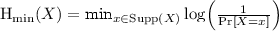 whereas the max-entropy is
  .
. - 4.
In fact, [DGRV11] show that the same conclusion holds even if we restrict the problem to constant-depth (i.e.,
 ) circuits.
 - 5.
Given such a scheme consider a circuit that has, hard-coded inside, a pair of ciphertexts \((c_0,c_1)\) which are either encryptions of the same bit or of different bits. The circuit gets as input a bit b and random string r and outputs a re-randomization of \(c_b\) (using randomness r). If the scheme is perfectly re-randomizing (and perfectly correct) then the min-entropy of the output distribution in case the plaintexts disagree is larger than the max-entropy in case the plaintexts agree.
- 6.
The hard distribution for \( \mathsf {SVP}_{\sqrt{n}} \) and \( \mathsf {CVP}_{\sqrt{n}} \) is the first message from the 2-message honest-verifier
 proof system of Goldreich and Goldwasser [GG98]. In the case of \( \mathsf {CVP}_{\sqrt{n}} \), the input is (B, t, d) where B is the basis of the lattice, t is a target vector and d specifies the bound on the distance of t from the lattice. The distribution is obtained by sampling a random error vector \( \eta \) from the ball of radius \( d\sqrt{n}/2 \) centered at the origin and outputting \( b\cdot t + \eta \mod \mathcal {P}(B) \), where
  and \( \mathcal {P}(B) \) is the fundamental parallelopiped of B. When t is far from the lattice, this distribution is injective and hence has high min-entropy while when t is close to the lattice, the distribution is not injective and hence has lower max-entropy. Similarly for \( \mathsf {SVP}_{\sqrt{n}} \), on input (B, d), the output is \( \eta \mod \mathcal {P}(B) \) where \( \eta \) is again sampled from a ball of radius \( d\sqrt{n}/2 \).
 - 7.
Note that the graph isomorphism is known to be solvable in polynomial-time for many natural distributions, and the recent breakthrough result of Babai [Bab16] gives a quasi-polynomial worst-case algorithm. Nevertheless, it is still plausible that Graph Isomorphism is average-case quasi-polynomially hard (for some efficiently samplable distribution).
- 8.
The trapdoor to the lossy function is not used in the construction of \( \mathsf {CRH}\).
- 9.
In contrast, it is easy to see that repetition amplifies the additive gap between the min-entropy and the max-entropy. In fact, we use this in our construction.
- 10.
- 11.
This setting (and construction) is similar to that of Peikert and Waters’s construction of \( \mathsf {CRH}\) from lossy functions [PW11].
- 12.
Recall that a collection of functions \(\mathcal {F}\) is k-wise independent if for every distinct \(x_1,\ldots ,x_k\), the distribution of \((f(x_1),\ldots ,f(x_k))\) (over the choice of \(f \leftarrow \mathcal {F}\)) is uniform.
- 13.
We remark that more efficient constructions are known, see Remark 2.4.
- 14.
We remark that our construction of \(\mathsf {MCRH}\) based on \(\mathsf {EA}_{\min ,\max }^{}\) (see Sect. 3) actually supports such large shrinkage.
- 15.
In a nutshell, the property that we are using is that if \(N=3^k\) balls are thrown into N bins, with high probability the maximal load in every bin will be at most \(\log (N)\). It is well-known that hash functions that are \(\log (N)\)-wise independent also have this property. See Sect. 2.2 for details.
- 16.
The general construction of statistically-hiding commitments from inaccessible entropy generators is meant to handle a much more general case than the one needed in our setting. In particular, a major difficulty handled by [HRVW09, HV17] is when the generator has many blocks and it is not known in which one there is a gap between the real and accessible entropies.
 .
. whereas the
  .
. ) circuits.
 proof system of Goldreich and Goldwasser [
 and
and  to a combination of [
References
Alon, N., Dietzfelbinger, M., Miltersen, P.B., Petrank, E., Tardos, G.: Linear hash functions. J. ACM 46(5), 667–683 (1999)
Applebaum, B., Raykov, P.: On the relationship between statistical zero-knowledge and statistical randomized encodings. In: Robshaw, M., Katz, J. (eds.) CRYPTO 2016. LNCS, vol. 9816, pp. 449–477. Springer, Heidelberg (2016). https://doi.org/10.1007/978-3-662-53015-3_16
Babai, L.: Graph isomorphism in quasipolynomial time [extended abstract]. In: Wichs, D., Mansour, Y. (eds.) Proceedings of the 48th Annual ACM SIGACT Symposium on Theory of Computing, STOC 2016, Cambridge, MA, USA, 18–21 June 2016, pp. 684–697. ACM (2016)
Berman, I., Degwekar, A., Rothblum, R.D., Vasudevan, P.N.: Multi collision resistant hash functions and their applications. IACR Cryptology ePrint Archive 2017, 489 (2017)
Bitansky, N., Paneth, O., Kalai, Y.T.: Multi-collision resistance: A paradigm for keyless hash functions. Electron. Colloquium Comput. Complex. (ECCC) 24, 99 (2017)
Brickell, E., Pointcheval, D., Vaudenay, S., Yung, M.: Design Validations for Discrete Logarithm Based Signature Schemes. In: Imai, H., Zheng, Y. (eds.) PKC 2000. LNCS, vol. 1751, pp. 276–292. Springer, Heidelberg (2000). https://doi.org/10.1007/978-3-540-46588-1_19
Elisa Celis, L., Reingold, O., Segev, G., Wieder, U.: Balls and bins: smaller hash families and faster evaluation. SIAM J. Comput. 42(3), 1030–1050 (2013)
Dvir, Z., Gutfreund, D., Rothblum, G.N., Vadhan, S.P.: On approximating the entropy of polynomial mappings. In: Proceedings of Innovations in Computer Science - ICS 2010, Tsinghua University, Beijing, China, 7–9 January 2011, pp. 460–475 (2011)
Ding, Y.Z., Harnik, D., Rosen, A., Shaltiel, R.: Constant-round oblivious transfer in the bounded storage model. J. Cryptol. 20(2), 165–202 (2007)
Dubrov, B., Ishai, Y.: On the randomness complexity of efficient sampling. In: Proceedings of the Thirty-Eighth Annual ACM Symposium on Theory of Computing, pp. 711–720. ACM (2006)
Damgård, I.B., Pedersen, T.P., Pfitzmann, B.: On the existence of statistically hiding bit commitment schemes and fail-stop signatures. In: Stinson, D.R. (ed.) CRYPTO 1993. LNCS, vol. 773, pp. 250–265. Springer, Heidelberg (1994). https://doi.org/10.1007/3-540-48329-2_22
Goldreich, O., Goldwasser, S.: On the limits of non-approximability of lattice problems. In: Proceedings of the Thirtieth Annual ACM Symposium on Theory of Computing, pp. 1–9. ACM (1998)
Goldwasser, S., Micali, S., Rivest, R.L.: A digital signature scheme secure against adaptive chosen-message attacks. SIAM J. Comput. 17(2), 281–308 (1988)
Girault, M., Stern, J.: On the length of cryptographic hash-values used in identification schemes. In: Desmedt, Y.G. (ed.) CRYPTO 1994. LNCS, vol. 839, pp. 202–215. Springer, Heidelberg (1994). https://doi.org/10.1007/3-540-48658-5_21
Goldreich, O., Sahai, A., Vadhan, S.: Can statistical zero knowledge be made non-interactive? or on the relationship of SZK and NISZK. In: Wiener, M. (ed.) CRYPTO 1999. LNCS, vol. 1666, pp. 467–484. Springer, Heidelberg (1999). https://doi.org/10.1007/3-540-48405-1_30
Haitner, I., Hoch, J.J., Reingold, O., Segev, G.: Finding collisions in interactive protocols—tight lower bounds on the round and communication complexities of statistically hiding commitments. SIAM J. Comput. 44(1), 193–242 (2015)
Halevi, S., Micali, S.: Practical and provably-secure commitment schemes from collision-free hashing. In: Koblitz, N. (ed.) CRYPTO 1996. LNCS, vol. 1109, pp. 201–215. Springer, Heidelberg (1996). https://doi.org/10.1007/3-540-68697-5_16
Haitner, I., Nguyen, M.-H., Ong, S.J., Reingold, O., Vadhan, S.P.: Statistically hiding commitments and statistical zero-knowledge arguments from any one-way function. SIAM J. Comput. 39(3), 1153–1218 (2009)
Hsiao, C.-Y., Reyzin, L.: Finding collisions on a public road, or do secure hash functions need secret coins? In: Franklin, M. (ed.) CRYPTO 2004. LNCS, vol. 3152, pp. 92–105. Springer, Heidelberg (2004). https://doi.org/10.1007/978-3-540-28628-8_6
Haitner, I., Reingold, O., Vadhan, S.P., Wee, H.: Inaccessible entropy. In: Proceedings of the 41st Annual ACM Symposium on Theory of Computing, STOC 2009, Bethesda, MD, USA, 31 May-2 June 2009, pp. 611–620 (2009)
Haitner, I., Vadhan, S.: The many entropies in one-way functions. Tutorials on the Foundations of Cryptography. ISC, pp. 159–217. Springer, Cham (2017). https://doi.org/10.1007/978-3-319-57048-8_4
Joux, A.: Multicollisions in iterated hash functions. Application to cascaded constructions. In: Franklin, M. (ed.) CRYPTO 2004. LNCS, vol. 3152, pp. 306–316. Springer, Heidelberg (2004). https://doi.org/10.1007/978-3-540-28628-8_19
Kilian, J.: A note on efficient zero-knowledge proofs and arguments (extended abstract). In: Proceedings of the 24th Annual ACM Symposium on Theory of Computing, Victoria, British Columbia, Canada, 4–6 May 1992, pp. 723–732 (1992)
Komargodski, I., Naor, M., Yogev, E.: Collision resistant hashing for paranoids: dealing with multiple collisions. IACR Cryptology ePrint Archive 2017, 486 (2017)
Komargodski, I., Naor, M., Yogev, E.: White-box vs. black-box complexity of search problems: ramsey and graph property testing. Electron. Colloquium Comput. Complex. (ECCC) 24, 15 (2017)
Merkle, R.C.: One way hash functions and DES. In: Brassard, G. (ed.) CRYPTO 1989. LNCS, vol. 435, pp. 428–446. Springer, New York (1990). https://doi.org/10.1007/0-387-34805-0_40
Micali, S.: Computationally sound proofs. SIAM J. Comput. 30(4), 1253–1298 (2000)
Meka, R., Reingold, O., Rothblum, G.N., Rothblum, R.D.: Fast pseudorandomness for independence and load balancing. In: Esparza, J., Fraigniaud, P., Husfeldt, T., Koutsoupias, E. (eds.) ICALP 2014. LNCS, vol. 8572, pp. 859–870. Springer, Heidelberg (2014). https://doi.org/10.1007/978-3-662-43948-7_71
Naor, M., Yung, M.: Universal one-way hash functions and their cryptographic applications. In: Proceedings of the 21st Annual ACM Symposium on Theory of Computing, Seattle, Washigton, USA, 14–17 May 1989, pp. 33–43 (1989)
Ostrovsky, R.: One-way functions, hard on average problems, and statistical zero-knowledge proofs. In: Proceedings of the Sixth Annual Structure in Complexity Theory Conference, Chicago, Illinois, USA, 30 June-3 July 1991, pp. 133–138 (1991)
Ong, S.J., Vadhan, S.: An equivalence between zero knowledge and commitments. In: Canetti, R. (ed.) TCC 2008. LNCS, vol. 4948, pp. 482–500. Springer, Heidelberg (2008). https://doi.org/10.1007/978-3-540-78524-8_27
Pietrzak, K., Rosen, A., Segev, G.: Lossy functions do not amplify well. In: Cramer, R. (ed.) TCC 2012. LNCS, vol. 7194, pp. 458–475. Springer, Heidelberg (2012). https://doi.org/10.1007/978-3-642-28914-9_26
Peikert, C., Waters, B.: Lossy trapdoor functions and their applications. SIAM J. Comput. 40(6), 1803–1844 (2011)
Rompel, J.: One-way functions are necessary and sufficient for secure signatures. In: Proceedings of the 22nd Annual ACM Symposium on Theory of Computing, Baltimore, Maryland, USA, 13–17 May 1990, pp. 387–394 (1990)
Rivest, R.L., Shamir, A.: Payword and micromint: two simple micropayment schemes. In: Proceedings of Security Protocols, International Workshop, Cambridge, United Kingdom, 10–12 April 1996, pp. 69–87 (1996)
Reingold, O., Trevisan, L., Vadhan, S.: Notions of reducibility between cryptographic primitives. In: Naor, M. (ed.) TCC 2004. LNCS, vol. 2951, pp. 1–20. Springer, Heidelberg (2004). https://doi.org/10.1007/978-3-540-24638-1_1
Rothblum, G.N., Vadhan, S.P.: Unpublished Manuscript (2009)
Simon, D.R.: Finding collisions on a one-way street: can secure hash functions be based on general assumptions? In: Nyberg, K. (ed.) EUROCRYPT 1998. LNCS, vol. 1403, pp. 334–345. Springer, Heidelberg (1998). https://doi.org/10.1007/BFb0054137
Vadhan, S.P.: Pseudorandomness. Found. Trends Theor. Comput. Sci. 7(1–3), 1–336 (2012)
Acknowledgments
We thank Vinod Vaikuntanathan for helpful discussions and for his support, and Oded Goldreich, Yuval Ishai and the anonymous reviewers for useful comments. We thank Nir Bitansky, Yael Kalai, Ilan Komargodski, Moni Naor, Omer Paneth and Eylon Yogev for helping us provide a good example of a t-way collision. We also thank Nir Bitansky and an anonymous reviewer for pointing out the connection to inaccessible entropy.
This research was supported in part by NSF Grants CNS-1413920 and CNS-1350619, and by the Defense Advanced Research Projects Agency (DARPA) and the U.S. Army Research Office under contracts W911NF-15-C-0226 and W911NF-15-C-0236. The third author was also partially supported by the SIMONS Investigator award agreement dated 6-5-12 and by the Cybersecurity and Privacy Institute at Northeastern University.
Author information
Authors and Affiliations
Corresponding author
Editor information
Editors and Affiliations
Rights and permissions
Copyright information
© 2018 International Association for Cryptologic Research
About this paper

Cite this paper
Berman, I., Degwekar, A., Rothblum, R.D., Vasudevan, P.N. (2018). Multi-Collision Resistant Hash Functions and Their Applications. In: Nielsen, J., Rijmen, V. (eds) Advances in Cryptology – EUROCRYPT 2018 . EUROCRYPT 2018. Lecture Notes in Computer Science(), vol 10821. Springer, Cham. https://doi.org/10.1007/978-3-319-78375-8_5
Download citation
DOI: https://doi.org/10.1007/978-3-319-78375-8_5
Published:
Publisher Name: Springer, Cham
Print ISBN: 978-3-319-78374-1
Online ISBN: 978-3-319-78375-8
eBook Packages: Computer ScienceComputer Science (R0)
