
Abstract
This chapter goes beyond the ELP theory of LCs by modeling the microstructure of the liquid by a number of rank-i tensors \((i=1, \ldots ,n)\) (generally just one) with vanishing trace. These tensors are called alignment tensors or order parameters. When formed as exterior products of the director vector and weighted with a scalar and restricted to just one rank-2 tensor, the resulting mathematical model describes uniaxial LCs. The simplest extensions of the ELP model are theories, for which the number of independent constitutive variables are complemented by a constant or variable order parameter S and its gradient \(\mathrm {grad}\,S\) paired with an evolution equation for it. We provide a review of the recent literature. Two different approaches to deduce LC models exist; they may be coined the balance equations models, outlined already in Chap. 25 for the ELP model, and the variational Lagrange potential models, which, following an idea by Lord Rayleigh (Strutt, Proc Lond Math Soc 4:357–368, 1873, [50]), are extended by a dissipation potential. The two different approaches may lead to distinct anisotropic fluid descriptions. Moreover, it is not automatically guaranteed in either description that the balance law of angular momentum is identically satisfied. The answers to these questions cover an important part of the mathematical efforts in both model classes. Significant conceptual difficulties in the two distinct theoretical concepts are the postulations of explicit forms of the elastic energy W and dissipation function R. Depending upon, how W and R are parametrized, different particular models emerge. Conditions are formulated especially for uniaxial models, which guarantee that the two model classes reduce to exactly corresponding mathematical models.
Access this chapter
Tax calculation will be finalised at checkout
Purchases are for personal use only
Notes
- 1.
- 2.
It turns out that the requirement of the existence of the Rayleigh dissipation potential corresponds to the assumption of the Onsager relations.
- 3.
With the aid of (26.15) we find in Cartesian coordinates \(x_{i}\) \((i=1,2,3)\) and \(x^{*}_{i^{*}}\) \((i^{*}=1,2,3)\)
$$\begin{aligned} \frac{\partial v^{*}_{i^{*}}}{\partial x^{*}_{j^{*}}}= & {} \frac{\partial }{\partial x^{*}_{j^{*}}} \left( Q_{i^{*}j} v_{j} + \dot{Q}_{i^{*}j} x_{j} + \dot{b}_{i^{*}}\right) = \frac{\partial }{\partial x_{k}}\left( Q_{i^{*}j} v_{j} + \dot{Q}_{i^{*}j} x_{j}+ \dot{b}_{i^{*}}\right) \underbrace{\frac{\partial x_{k}}{\partial x^{*}_{j^{*}}}}_{Q_{j^{*}k}} \\= & {} \left( Q_{i^{*}j }\frac{\partial v_{j}}{\partial x_{k}} + \dot{Q}_{i^{*}k}\right) Q_{j^{*}k} = \underline{Q_{i^{*}j}\frac{\partial v_{j}}{\partial x_{k}}Q_{j^{*}k}+\dot{Q}_{i^{*}k} Q_{j^{*}k}}\,, \\ \frac{\partial v_{j}^{*}}{\partial x_{i^{*}}}= & {} Q_{j^{*}j} \frac{\partial v_{j}}{\partial x_{k}} Q_{i^{*}k} + \dot{Q}_{j^{*}k}Q_{i^{*}k} {\mathop {=}\limits ^{j \leftrightarrow k}} Q_{j^{*}k} \frac{\partial v_{k}}{\partial x_{j}} Q_{i^{*}j} + \underbrace{ \dot{Q}_{j^{*}k} Q_{i^{*}k}}_{-Q_{j^{*}k} \dot{Q}_{i^{*}k}} \\= & {} Q_{i^{*}j}\frac{\partial v_{k}}{\partial x_{j}} Q_{j^{*}k} - \dot{Q}_{i^{*}k} Q_{j^{*}k} = \underline{ Q_{i^{*}j} \frac{\partial v_{k}}{\partial x_{j}} Q_{j^{*}k} + \dot{Q}_{j^{*}k}Q_{i^{*}k} } \, . \end{aligned}$$The underbraced term follows from \(Q_{i^{*}k}Q_{j^{*}k} = \delta _{i^{*}j^{*}}\) and relations (26.16) are immediate consequences of the underlined terms.
- 4.
This statement is restricted to those models satisfying the Onsager relations; this is so, because the existence of a dissipation potential as in the Lagrange–Rayleigh formulation exactly corresponds to the application of the Onsager relations.
- 5.
This fact is informative and the introductory text in [44] is worth reading. However, in this electronic time, we refrain from copying it.
- 6.
- 7.
Let f(xy) be a homogeneous function of order \({\varvec{n}}\) so that

Then, it is easy to show that
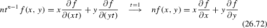
for a homogeneous function of order n. For a bilinear homogeneous function \( n=2\).
- 8.
For a brief biographical sketch of Pierre-Gilles De Gennes (1932–2007), see Fig. 26.1 .
- 9.
\(RHS(\cdot )\) and \(LHS(\cdot )\) denote the right- and left-hand sides of the equation \((\cdot )\).
- 10.
We will show that for the choice of the function W the first of the underlined terms will be symmetric.
- 11.
In these tables, the first line shows those combinations of \({\mathop {{\varvec{Q}}}\limits ^{\circ }}\) and \({\varvec{D}}\) which do not involve \({\varvec{Q}}\). The remaining four lines then show those scalar invariants, which are combinations with linear or quadratic \({\varvec{Q}}\)-dependences. We shall identify the 15 elements of these tables by the indices
$$\begin{array}{l@{\quad }l@{\quad }l@{\quad }l@{\quad }l} \hline \,[1] &{}&{} [2] &{}&{} [3] \\ \hline \,[11] &{} &{} [21] &{} &{} [31] \\ \,[12] &{}&{} [22] &{}&{} [32] \\ \,[13] &{}&{} [23] &{}&{} [33] \\ \,[14] &{} &{} [24] &{} &{} [34] \\ \hline \end{array}$$ - 12.
- 13.
The term “holonomic” was introduced by Heinrich Hertz in 1894 from the Greek “\(\breve{o}\lambda \)o\(\varsigma \)” (whole, entire) and “\(\nu \)ó\(\mu \)o\(\varsigma \)” (law).
- 14.
Reshuffling indices means that the name of a doubly repeated index may be changed at liberty to possibly reach a formula that might formally agree with some other formula.


References
Ajdari, A.: Pierre-Gilles de Gennes (1932–2007). Science 317(5837), 466 (2007). https://doi.org/10.1126/science.1146688
Beris, A.N., Edwards, B.J.: Thermodynamics of Flowing Systems with Internal Microstructure. Oxford Engineering Science Series, vol. 36. Oxford University Press, New York (1994)
Carlsson, T., Leslie, F.M., Laverty, J.S.: Flow properties of biaxial nematioc liquid crystals. Mol. Cryst. Liq. Cryst. 210, 95–127 (1992)
Capriz, G.: Continua with Microstructure. Springer, New York (1989)
de Gennes, P.G.: Short range order effects in the isotropic phase of nematics and cholesterics. Mol. Cryst. Liq. Cryst. 12, 193–214 (1971)
de Gennes, P.G.: Scaling Concepts in Polymer Physics. Cornell University Press, Ithaca (1979). ISBN 0-8014-1203-X
de Gennes, P.G., Prost, J.: The Physics of Liquid Crystals. Clarendon Press, Oxford (1993). ISBN 0-19-852024-7
de Gennes, P.G., Brochard-Wyart, F., Quéré, D.: Capillarity and Wetting Phenomena: Drops, Bubbles, Pearls, Waves. Springer, Berlin (2003). ISBN 0-387-00592-7
Diogo, A.C., Martins, A.F.: Order parameter and temperature dependence of the hydrodynamic viscosities of nematics liquid crystals. Journal de Physique 43, 779–782 (1972)
Doi, M.: Molecular dynamics and rheological properties of concentrated solutions of rodlike polymers in isotropic and liquid crystalline phases. J. Polym. Sci. Polym. Phys. 19(2), 229–243 (1981)
Ehrentraut, H.: A unified mesoscopic continuum theory of uniaxial and biaxial liquid crystals. Ph.D. thesis, TU Berlin, Department of Physics (1996)
Ericksen, J.L.: Conservation laws for liquid crystals. Trans. Soc. Rheol. 5, 23–34 (1961)
Ericksen, J.L.: Hydrostatic theory of liquid crystals. Arch. Ration. Mech. Anal. 21, 371–378 (1962)
Ericksen, J.L.: On equations of motion for liquid crystals. Quart. J. Mech. Appl. Math. 29, 203–208 (1976)
Ericksen, J.L.: Liquid crystals with variable degree of orientation. Arch. Ration. Mech. Anal. 113, 97–120 (1991)
Faraoni, V., Grosso, M., Crescitelli, S., Maffettone, P.L.: The rigid rod model for neematic polymers: an analysis of the shear problem. J. Rheol. 43, 829–843 (1999)
Forster, D.: Microscopic theory of flow alignment in nematic liquid crystals. Phys. Rev. Lett. 32, 1161 (1974)
Green, A.E., Rivlin, R.S.: Simple force and stress multipoles. Arch. Ration. Mech. Anal. 16, 325–354 (1964)
Green, A.E., Naghdi, P.M., Rivlin, R.S.: Directors and multipolar displacements in continuum mechanics. Int. J. Eng. Sci. 2, 611–620 (1965)
Grosso, M., Maffettone, P.L., Dupret, F.: A closure approximation for nematic liquid crystals based on the canonical distribution subspace theory. Rheol. Acta 39, 301–310 (2000)
Hess, S.: Irreversible thermodynamics of non-equilibrium alignment phenomena in molecular liquids and in liquid crystals. Z. Naturforsch. 30a, 728 (1975)
Hess, S.: Pre- and post-transitional behavior of the flow alignment and flow-induced phase transition in liquid crystals. Z. Naturforsch. 31a, 1507–1513 (1976)
Hess, S.: Transport phenomena in anisotropic fluids and liquid crystals. J. Non-Equilib. Thermodyn. 11, 175–193 (1986)
Hess, S., Pardowitz, Z.: On the unified theory for non-equilibrium phenomena in the isotropic and nematic phases of a liquid crystal – spatially homogeneous alignment. Z. Naturforsch. 36a, 554–558 (1981)
Hutter, K., Jöhnk, K.: Continuum Methods of Physical Modeling, 635 pp. Springer, Berlin (2004)
Leslie, F.M.: Some constitutive equations for anisotropic fluids. Quart. J. Mech. Appl. Math. 19, 357–370 (1966)
Leslie, F.M.: Some constitutive equations for liquid crystals. Arch. Ration. Mech. Anal. 28, 265–283 (1968)
Leslie, F.M.: Continuum theory for nematic liquid crystals. Contin. Mech. Thermodyn. 4, 167–175 (1992)
Leslie, F.M., Laverty, J.S., Carlsson, T.: Continuum theory of biaxial nematic liquid crystals. Quart. J. Mech. Appl. Math. 45, 595–606 (1992)
Maffettone, P.L., Sonnet, A.M., Virga, E.G.: Shear-induced biaxiality in nematic polymers. J. Non-Newton. Fluid Mech. 90, 283–297 (2000)
Maier, W., Saupe, A.: Eine einfache molecular-statistische Theorie der nematischen kristallflüssigen Phase. Zeitschrift für Naturforschung A 14(10), 882–889 (1959). https://doi.org/10.1515/zna-1959-10005
Marrucci, G.: Prediction of Leslie coefficients fior rodlike polymer nematics. Mol. Cryst. Liq. Cryst. (Lett.) 72, 153–161 (1982)
Marrucci, G.: The Doi-Edwards model in slow flow. Predictions on the Weissenberg effect. J. Non-Newton. Fluid Mech. 21(3), 319–328 (1986)
Moffettone, P.L., Sonnet, A.M., Virga, E.G.: Shear-induced bi-axiality in nematics polymers. J. Non-Newton. Fluid Mech. 90, 283–297 (2000)
Olmsted, P.D., Goldbart, P.: Theory of the nonequilibrium phase transition for nematic liquid crystals under shear flow. Phys. Rev. A 41, 4578–4581 (1990)
Olmsted, P.D., Goldbart, P.: Isotropic-nematic transition in shear flow: state selection, coexistence, phase transitions, and critical behavior. Phys. Rev. A 46, 4966–4993 (1992)
Parodi, O.: Stress tensor for a nematic liquid crystal. Le journal de Physque 31, 581–584 (1970)
Pereira-Borgmeyer, C., Hess, S.: Unified description of the flow alignment and viscosity in the isotropic and nematic phases of liquid crystals. J. Non-Equilib. Thermodyn. 20, 359–384 (1995)
Qian, T., Sheng, P.: Generalized hydrodynamic equations for nematic liquid crystals. Phys. Rev. E 58, 7475 (1998)
Rienaecker, G., Hess, S.: Oriental dynamics of nematics liquid crystals under a shear flow. Phys. A 267, 294–321 (1999)
Saupe, A.: Das Protonenresonanzspektrum von orientiertem Benzol in nematisch-kristallinflüssiger Lösung. Z. Naturforsch. 20a, 572–580 (1965)
Singh, A.P., Rey, A.D.: Theory and simuation of extensional flow-induced biaxiality in duiscotic mesophases. Journal de Physique II(5), 1321–1348 (1995)
Smith, G.E.: On isotropic integrity bases. Arch. Ration. Mech. Anal. 18, 282–292 (1965)
Sonnet, A.M., Virga, E.G.: Dynamics of dissipative ordered fluids. Phys. Rev. E 64(3), 031705-1-10 (2001)
Sonnet, A.M., Maffettone, P.L., Virga, E.G.: Dissipative Ordered Fluid: Theories for Liquid Crystals. Springer Science & Business Media LLC, New York (2012)
Sonnet, A.M., Maffettone, P.L., Virga, E.G.: Continuum theory for nematic liquid crystals with tensorial order. J. Non-Newton. Fluid Mech. 119, 51–59 (2004)
Spencer, A.J.M.: Theory of invariants. In: Eringen, A.C. (ed.) Continuum Physics: Volume 1–Mathematics, pp. 239–353. Academic Press, New York (1971)
Stephen, M.J., Straley, J.P.: Physics of liquid crystals. Rev. Mod. Phys. 46(4), 617–703 (1974). https://doi.org/10.1007/BF01516710
Stark, H., Lubensky, T.C.: Poisson-bracket approach to the dynamics of nematic liquid crystals - The role of spin angular momentum. Phys. Rev. E 72, 051714 (2005)
Strutt, J.W.: (Lord Rayleigh): some general theorems relating to vibrations. Proc. Lond. Math. Soc. 4, 357–368 (1873)
Vertogen, G.: The equations of motion for nematics. Z. Naturforsch. 38a, 1273 (1983)
Wang, C.C.: A new representation for isotropic functions. Parts I and II. Arch. Ration. Mech. Anal. 36(166–197), 198–223 (1970)
Wang, C.C.: Corrigendum to my recent paper on ‘Representations for isotropic functions’. Arch Ration. Mech. Anal. 43, 392–395 (1971)
Whittaker, E.T.: A Treatize on the Analytical Dynamics of Particles and Rigid Bodies, 4th edn. Cambridge University Press, Cambridge (1937)
Author information
Authors and Affiliations
Corresponding author
Appendices
Appendix 26.A Lagrange Equations
26.1.1 26.A.1 Constraints of Coordinates
Consider a mechanical system (e.g., of mass points \({\mathcal P}_{i}\) \(i=1,2, \ldots ,n\)) whose motion can be determined by prescribing their coordinates \(\{{\varvec{x}}_{1}, {\varvec{x}}_{2}, \ldots , {\varvec{x}}_{n} \}\) see Fig. 26.2 . The degree of freedom of a mechanical system is the number of independent coordinates needed to describe the motion of the system. Constraints or constraint conditions are equations between coordinates, which restrain the motion of the system. Rigid point systems with constants of the form
express rigid body motions. They have six degrees of freedom, three for translation and three for rotation. In analytical dynamics, one differentiates between two kinds of constraint conditions.
(i) Constraint conditions, which are expressible as equations between coordinates, are called holonomic.Footnote 13
(ii) If constraints are not expressible in holonomic form, they are called anholonomic or skleronomic . If such a constraint condition is not explicitly expressible as a function also of time it is called skleronomic, else rheonomic .

System of n mass points in \({\mathbb R}^{3}\) with positions \({\varvec{x}}_{i}\) \(i=1, 2, \ldots ,n\) and distances \(r_{ij}\)
26.1.2 26.A.2 Generalized Coordinates
When holonomic constraints exist between the coordinates \(\{{\varvec{x}}_{1}, {\varvec{x}}_{2}, \ldots , {\varvec{x}}_{n}\}\), these constraint conditions will reduce the degree of freedom. If these \(\varLambda \) equations are independent of one another, the degree of freedom f will be \(f = 3n - \varLambda \). In this case, the mechanical system can be described by the so-called generalized coordinates
In other words, these coordinates determine the values of \(\{{\varvec{x}}_{1}, \ldots ,{\varvec{x}}_{n}\}\) uniquely as functions of time as follows:
These are 3n transformation equations between the dependent coordinates \(\{x_{i}, y_{i}, z_{i}\}\) \(i=1, 2, \ldots , n\) and the independent generalized coordinates \(\{q_{1}, \ldots ,q_{f}\}\). Their total time derivatives \(\{\dot{q}_{1}, \ldots , \dot{q}_{f}\}\) are called generalized velocities.
26.1.3 26.A.3 d’Alembert’s Principle, Principle of Virtual Work
A virtual displacement of \(\{{\varvec{x}}_{i}\) \(i=1, \ldots ,n\}\) of a mechanical system is a set \(\{\delta {\varvec{x}}_{i}\) \(i=1, \ldots ,n\}\) of instantaneous infinitesimal changes of the positions \(\{{\varvec{x}}_{i}\) \(i=1, \ldots ,n\}\) which are consistent with the existing forces and constraints. Here, the qualification “instantaneous” wants to emphasize that the displacement is performed, while the time is held fixed; this displacement is called “consistent with the applied forces and with the constraints,” because these displacements are kinematically force-freely admissible. Often, one also speaks of virtual velocities. This then leads to the Principle of Virtual Power . To derive it, let us start with the momentum equation in the form
in which \({\varvec{F}}_{i}\) are the external and internal forces and \(p_{i}\) is the momentum corresponding to \({\varvec{F}}_{i}\). Multiplying both sides of (26.194) scalarly with \(\delta {\varvec{x}}_{i}\) and summation over all indices \(1, \ldots ,n\) yields
In general, \({\varvec{F}}_{i}\) is the sum of the applied force \({\varvec{F}}_{i}^{(a)}\) and the constraint force \({\varvec{F}}_{i}^{(c)}\)
The decisive additional assumption for the elimination of the constraint forces from the problem is the postulate that the virtual work of the constraint forces is null,
This equation is the expression of the Principle of Virtual Work , or when expressed in virtual velocities the Principle of Virtual Power .
Combining (26.195) with (26.196), (26.197) yields
This is known as d’Alembert’s Principle .
26.1.4 26.A.4 Derivation of the Lagrange Equations
Consider now virtual displacements of the generalized coordinates \(\delta {\varvec{q}}_{i}\) \((i=1, \ldots ,f)\). If the functions (26.193) are differentiable, which we will assume, we may write
A differentiation with respect to time is missing in this expression because the virtual displacements are instantaneously performed. Substitution of (26.199) into d’Alembert’s Principle yields with \(\dot{{\varvec{p}}}_{i}= m_{i} \ddot{{\varvec{x}}}_{i}\)
Remarks:
-
The quantity
$$\begin{aligned} Q_{j} : = \sum _{i=1}^{n} {\varvec{F}}_{i} \cdot \frac{\partial {\varvec{x}}_{i}}{\partial q_{j}} \quad (j=1, \ldots ,f) \end{aligned}$$(26.201)is known as jth generalized force .
-
The reader can easily verify the following formulae:
-
(1)
$$\begin{aligned} {\varvec{v}}_{i} = \dot{\varvec{x}}_{i} = \sum _{j=1}^{f}\frac{\partial {\varvec{x}}_{i}}{\partial q_{j}} \dot{q}_{j} + \frac{\partial {\varvec{x}}_{i}}{\partial t}\quad \Longrightarrow \quad \frac{\partial {\varvec{v}}_{i}}{\partial \dot{q}_{j} }= \frac{\partial {\varvec{x}}_{i}}{\partial q_{j}}, \end{aligned}$$(26.202)
-
(2)
$$\begin{aligned} \frac{\mathrm {d}}{\mathrm {d} t}\left( \frac{\partial {\varvec{x}}_{i}}{\partial q_{j}}\right)= & {} \sum _{k}\frac{\partial ^{2} {\varvec{x}}_{i}}{\partial q_{j} \partial q_{k}} \dot{q}_{k} + \frac{\partial ^{2}{\varvec{x}}_{i}}{\partial q_{j} \partial t} \nonumber \\= & {} \frac{\partial }{\partial q_{j}}\left( \sum _{k}\frac{\partial {\varvec{x}}_{i}}{\partial q_{k}} \dot{q}_{k} + \frac{\partial {\varvec{x}}_{i}}{\partial t}\right) =\frac{\partial {\varvec{v}}_{i}}{\partial q_{j}} , \end{aligned}$$(26.203)
-
(3)
$$\begin{aligned}&\sum _{ij}m\ddot{{\varvec{x}}}_{i}\cdot \frac{\partial {\varvec{x}}_{i}}{\partial q_{j}} \delta q_{j} \nonumber \\= & {} \sum _{i,j}\left\{ \frac{\mathrm {d}}{\mathrm {d}t}\left( \frac{\partial }{\partial \dot{q}_{j}} \frac{m_{i} {\varvec{v}}_{i}\cdot {\varvec{v}}_{i}}{2} \right) - \frac{\partial }{\partial q_{j}} \left( \frac{m_{i} {\varvec{v}}_{i}\cdot {\varvec{v}}_{i}}{2}\right) \right\} \delta {q}_{j} \nonumber \\= & {} \sum _{j}\left\{ \frac{\mathrm {d}}{\mathrm {d}t}\left( \frac{\partial }{\partial \dot{q}_{j}} \frac{\sum _{i} m_{i}{\varvec{v}}_{i}\cdot {\varvec{v}}_{i}}{2}\right) - \frac{\partial }{\partial q_{j}} \left( \frac{\sum _{i}m_{i} {\varvec{v}}_{i} \cdot {\varvec{v}}_{i}}{2}\right) \right\} \delta {q}_{j} \nonumber \\= & {} \sum _{j}\left\{ \frac{\mathrm {d}}{\mathrm {d}t}\left( \frac{\partial T}{\partial \dot{q}_{j}}\right) - \frac{\partial T}{\partial q_{j}}\right\} \delta q_{j} , \end{aligned}$$(26.204)
where T is the kinetic energy.
-
(1)
Substituting (26.201)–(26.204) into (26.200) d’Alembert’s Principle leads to
Consequently,
These equations are sometimes called the Lagrange equations. Regularly, this denotation is, however, only used, if the forces \({\varvec{F}}_{i}\) are derivable from a potential \(V(q_{1}, \ldots , q_{f},t) = V({\varvec{x}}_{1}, {\varvec{x}}_{2}, \ldots , {\varvec{x}}_{n})\) according to
The generalized forces can then be written as
Introducing the Lagrange function
and using (26.208) and the fact that V does not depend upon \(\dot{q}_{i}\) we deduce from (26.205)
or
which is equivalent to (26.206).
Example: Consider a pearl with mass m tied to a vertical circular wire, which rotates with constant angular velocity \(\omega \) around a vertical axis, see Fig. 26.3 . The pearl can freely move along the wire. Let the radius of the circle of the wire be R and let the gravity vector in the vertical plane be \({\varvec{g}}\) positive downward. The motion of the pearl can be described by the angle \(\varphi \). So, this angle serves as the only generalized coordinate. For the pearl, treated as a mass point, we have

Pearl moving on a permanently rotating circular wire
Because the system has only one degree of freedom, we have only a single Lagrange equation:
Substituting these expressions into the Lagrange Equation (26.210) yields
which is the solution of the equation of motion.
Appendix 26.B Implications of the Frame Indifference Requirement of the Free Energy as a Function of Tensorial Order Parameters
Let W be the free energy. In the main text, it is assumed to be a function of the director \({\varvec{n}}\) and its gradient, \(\mathrm {grad}\,{\varvec{n}}\). Satisfaction of the frame indifference requirement has been expressed as the statement (26.45) or (26.46). If W depends on a set of rank-i tensors \((i=2, \ldots ,n)\) its frame indifference is expressed as Eq. (26.44). Here, we begin with a W-function that depends only on a rank-2 tensor and its gradient: \(W = W(\pmb {\mathbb O}, \mathrm {grad}\,\pmb {\mathbb O})\). Invariance of W under Euclidian transformations (rigid body motions) then implies
in which
\({\varvec{R}}\) is an orthogonal transformation [\({\varvec{R}}{\varvec{R}}^{T}={\varvec{I}}\)]. Cartesian tensor notation is used with indices \(i, j, k, \ldots \) and \(i^{*}, j^{*}, k^{*}, \ldots \) in the original and in the rotated coordinates, respectively. \({\varvec{x}}^{*}\) is the position of the point \({\varvec{x}}\) measured in the rotated coordinates given by \({\varvec{R}}\) and translation by \({\varvec{b}}^{*}\). Below we shall restrict attention to infinitesimal rotations,
for which only linear terms in \({\varvec{\varOmega }}\) are accounted for. It is then easily shown that
Our next step is evaluation of \(\pmb {\mathbb O}\) and \(\mathrm {grad}\,\pmb {\mathbb O}\) in the rotated coordinates:
-
$$\begin{aligned} {\mathbb O}_{i^{*}j^{*}}= & {} R_{i^{*}m} R_{j^{*}m} {\mathbb O}_{mn} = (\delta _{i^{*}m}+\varOmega _{i^{*}m})(\delta _{j^{*}m}+\varOmega _{j^{*}m}) {\mathbb O}_{mn}\nonumber \\= & {} \left( \delta _{i^{*}m}\delta _{j^{*}m}+\delta _{i^{*}m}\varOmega _{j^{*}n}+ \delta _{j^{*}n}\varOmega _{i^{*}m}\right) {\mathbb O}_{mn} \nonumber \\= & {} {\mathbb O}_{i^{*}j^{*}}+{\mathbb O}_{i^{*}n}\varOmega _{j^{*}n} +{\mathbb O}_{m j^{*}}\varOmega _{i^{*}m}, \end{aligned}$$(26.216)
-
$$\begin{aligned} {\mathbb O}_{i^{*}j^{*}, k^{*}}= & {} R_{i^{*}m} R_{j^{*}n} {\mathbb O}_{mn,k} \frac{\partial x_{k}}{\partial x^{*}_{k^{*}}}{\mathop {=}\limits ^{({6.B2})}} R_{i^{*}m} R_{j^{*}n}R_{k^{*}k}{\mathbb O}_{mn,k} \nonumber \\= & {} \left( \delta _{i^{*}m}\delta _{j^{*}m} + \delta _{i^{*}m} \varOmega _{j^{*}n} + \delta _{j^{*}n}\varOmega _{i^{*}m}\right) \left( \delta _{k^{*} k} + \varOmega _{k^{*}k}\right) {\mathbb O}_{mn, k} \nonumber \\= & {} \left( \delta _{i^{*}m}\delta _{j^{*}n}\delta _{k^{*}k} + \delta _{i^{*} m} \delta _{k^{*} k} \varOmega _{j^{*}n}\right. \nonumber \\&\left. + \delta _{j^{*} n} \delta _{k^{*} k} \varOmega _{i^{*}m}\varOmega _{i^{*}m} + \delta _{i^{*}m}\delta _{j^{*}n}\varOmega _{k^{*} k}\right) {\mathbb O}_{mn, k} \nonumber \\= & {} {\mathbb O}_{i^{*}j^{*},k^{*}} + {\mathbb O}_{i^{*}n,k^{*}}\varOmega _{j^{*}n} + {\mathbb O}_{m j^{*},k^{*}}\varOmega _{i^{*}m} \nonumber \\&+ {\mathbb O}_{i^{*} j^{*},k^{*}}\varOmega _{k^{*}k} .\qquad \end{aligned}$$(26.217)
With the normalization \(W({\mathbb O}_{ij}=0\) \({\mathbb O}_{ij,k}=0)=0\) and employing first-order Taylor series expansion one may write
This expression is linear in the skew-symmetric rank-2 tensor \({\varvec{\varOmega }}\) and can be written in the following new form by reshuffling indices.Footnote 14 Such a reshuffling yields
Because the tensor \(\varOmega _{k^{*} k}\) is skew-symmetric, the rank-2 tensor \(F_{k^{*} k}\) in the curly bracket of this expression must be symmetric, or its skew-symmetric part must vanish. This can be expressed as \(\varepsilon _{p k^{*} k}F_{k^{*} k}= 0\) or
Introducing the multi-indices I and \(I_{k ^{j}}\) as defined in (26.14), this expression can alternatively be written as
Sonnet and Virga [44] must have performed the analogous computation for a free energy function W which is a function of a finite number of rank-i tensors \(\pmb {\mathbb O}\) (\(i = 1,2, \ldots ,n\)). The frame indifference postulate is then Eq. (26.44). Invariance of W under an infinitesimal rigid body rotation is then expressible as a statement analogous to (26.219), explicitly as
With the above proof of the frame indifference as a function of the rank-2 order parameters \(\pmb {\mathbb O}\), it is quite natural, how (26.221) can be proven, e.g., by the reader.
Appendix 26.C Euclidian Invariance of \({\mathop {{\varvec{Q}}}\limits ^{\diamond }}\)
We prove here the frame indifference of the co-deformational derivative of the rank-2 order parameter

where \(\sigma \) is a scalar constitutive parameter or a constant. Let \({\varvec{R}}\) be an orthogonal second rank tensor, so that \({\varvec{R}}{\varvec{R}}^{T} = {\varvec{I}}\). Note, moreover, that \({\varvec{Q}}\) is a deviator by definition. Then

which demonstrates objectivity of the quantity \(({\cdot })\) in (26.223). Next,

demonstrating Euclidian invariance of the last term on the right-hand side of (26.223). It follows that the co-deformational derivative of \({\varvec{Q}}\) is an objective rank-2 tensor.
Rights and permissions
Copyright information
© 2018 Springer International Publishing AG, part of Springer Nature
About this chapter

Cite this chapter
Hutter, K., Wang, Y. (2018). Nematic Liquid Crystals with Tensorial Order Parameters. In: Fluid and Thermodynamics. Advances in Geophysical and Environmental Mechanics and Mathematics. Springer, Cham. https://doi.org/10.1007/978-3-319-77745-0_26
Download citation
DOI: https://doi.org/10.1007/978-3-319-77745-0_26
Published:
Publisher Name: Springer, Cham
Print ISBN: 978-3-319-77744-3
Online ISBN: 978-3-319-77745-0
eBook Packages: Earth and Environmental ScienceEarth and Environmental Science (R0)