A Glimpse of Young Tableaux

Abstract

We defined in Chapter 6 Young’s lattice Y , the poset of all partitions of all nonnegative integers, ordered by containment of their Young diagrams.

We defined in Chapter 6 Young’s lattice Y , the poset of all partitions of all nonnegative integers, ordered by containment of their Young diagrams.

Here we will be concerned with the counting of certain walks in the Hasse diagram (considered as a graph) of Y . Note that since Y  is infinite, we cannot talk about its eigenvalues and eigenvectors. We need different techniques for counting walks. It will be convenient to denote the length of a walk by n, rather than by ℓ as in previous chapters.

Note that Y  is a graded poset (of infinite rank), with Y _i consisting of all partitions of i. In other words, we have Y = Y ₀ ⋅ ∪Y ₁ ⋅ ∪⋯ (disjoint union), where every maximal chain intersects each level Y _i exactly once. We call Y _i the ith level of Y , just as we did for finite graded posets.

Since the Hasse diagram of Y  is a simple graph (no loops or multiple edges), a walk of length n is specified by a sequence λ ⁰, λ ¹, …, λ ⁿ of vertices of Y . We will call a walk in the Hasse diagram of a poset a Hasse walk. Each λ ⁱ is a partition of some integer, and we have either (a) λ ⁱ < λ ⁱ⁺¹ and |λ ⁱ| = |λ ⁱ⁺¹|− 1, or (b) λ ⁱ > λ ⁱ⁺¹ and |λ ⁱ| = |λ ⁱ⁺¹| + 1. (Recall that for a partition λ, we write |λ| for the sum of the parts of λ.) A step of type (a) is denoted by U (for “up,” since we move up in the Hasse diagram), while a step of type (b) is denoted by D (for “down”). If the walk W has steps of types A ₁, A ₂, …, A _n , respectively, where each A _i is either U or D, then we say that W is of type A _n A _n−1⋯A ₂ A ₁. Note that the type of a walk is written in the opposite order to that of the walk. This is because we will soon regard U and D as linear transformations, and we multiply linear transformations right-to-left (opposite to the usual left-to-right reading order). For instance (abbreviating a partition (λ ₁, …, λ _m ) as λ ₁⋯λ _m ), the walk ∅, 1, 2, 1, 11, 111, 211, 221, 22, 21, 31, 41 is of type UUDDUUUUDUU = U ² D ² U ⁴ DU ².

There is a nice combinatorial interpretation of walks of type U ⁿ which begin at ∅. Such walks are of course just saturated chains $\emptyset =\lambda ^0\lessdot \lambda ^1\lessdot \cdots \lessdot \lambda ^{n}$. In other words, they may be regarded as sequences of Young diagrams, beginning with the empty diagram and adding one new square at each step. An example of a walk of type U ⁵ is given by

We can specify this walk by taking the final diagram and inserting an i into square s if s was added at the ith step. Thus the above walk is encoded by the “tableau”

Such an object τ is called a standard Young tableaux (or SYT). It consists of the Young diagram D of some partition λ of an integer n, together with the numbers 1, 2, …, n inserted into the squares of D, so that each number appears exactly once, and every row and column is increasing. We call λ the shape of the SYT τ, denoted λ = sh(τ). For instance, there are five SYT of shape (2, 2, 1), given by

Let f ^λ denote the number of SYT of shape λ, so for instance f ^{(2, 2, 1)} = 5. The numbers f ^λ have many interesting properties; for instance, there is a famous explicit formula for them known as the Frame–Robinson–Thrall hook length formula. For the sake of completeness we state this formula without proof, though it is not needed in what follows.

Let u be a square of the Young diagram of the partition λ. Define the hook H(u) of u (or at u) to be the set of all squares directly to the right of u or directly below u, including u itself. The size (number of squares) of H(u) is called the hook length of u (or at u), denoted h(u). In the diagram of the partition (4, 2, 2) below, we have inserted the hook length h(u) inside each square u.

FormalPara 8.1 Theorem (Hook Length Formula)

Let λ ⊢ n. Then

$$\displaystyle \begin{aligned} f^\lambda = \frac{n!}{\prod_{u\in\lambda}h(u)}. \end{aligned}$$

Here the notation u ∈ λ means that u ranges over all squares of the Young diagram of λ.

For instance, the diagram of the hook lengths of λ = (4, 2, 2) above gives

$$\displaystyle \begin{aligned} f^{(4,2,2)} = \frac{8!}{6\cdot 5\cdot 2\cdot 1\cdot 3\cdot 2\cdot 2\cdot 1} = 56. \end{aligned}$$

In this chapter we will be concerned with the connection between SYT and counting walks in Young’s lattice. If w = A _n A _n−1⋯A ₁ is some word in U and D and λ ⊢ n, then let us write α(w, λ) for the number of Hasse walks in Y  of type w which start at the empty partition ∅ and end at λ. For instance, α(UDUU, 11) = 2, the corresponding walks being ∅, 1, 2, 1, 11 and ∅, 1, 11, 1, 11. Thus in particular α(U ⁿ, λ) = f ^λ [why?]. In a similar fashion, since the number of Hasse walks of type D ⁿ U ⁿ which begin at ∅, go up to a partition λ ⊢ n, and then back down to ∅ is given by (f ^λ)², we have

$$\displaystyle \begin{aligned} \alpha(D^nU^n, \emptyset) = \sum_{\lambda\vdash n}(f^{\lambda})^2. {} \end{aligned} $$

(8.1)

Our object is to find an explicit formula for α(w, λ) of the form f ^λ c _w , where c _w does not depend on λ. (It is by no means a priori obvious that such a formula should exist.) In particular, since f ^∅ = 1, we will obtain by setting λ = ∅ a simple formula for the number of (closed) Hasse walks of type w from ∅ to ∅ (thus including a simple formula for (8.1)).

There is an easy condition for the existence of any Hasse walk of type w from ∅ to λ, given by the next lemma.

FormalPara 8.2 Lemma

Suppose $w = D^{s_k}U^{r_k}\cdots D^{s_2}U^{r_2}D^{s_1}U^{r_1}$ , where r _i  ≥ 0 and s _i  ≥ 0. Let λ ⊢ n. Then there exists a Hasse walk of type w from ∅ to λ if and only if:

$$\displaystyle \begin{aligned} \sum_{i=1}^{k} (r_i-s_i) = n \end{aligned}$$

$$\displaystyle \begin{aligned} \sum_{i=1}^{j} (r_i-s_i) \geq 0 \mathit{\mbox{ for }}1\leq j \leq k. \end{aligned}$$

FormalPara Proof

Since each U moves up one level and each D moves down one level, we see that $\sum _{i=1}^{k} (r_i-s_i)$ is the level at which a walk of type w beginning at ∅ ends. Hence $\sum _{i=1}^{k} (r_i-s_i) = |\lambda | = n$.

After $\sum _{i=1}^{j}(r_i+s_i)$ steps we will be at level $\sum _{i=1}^{j} (r_i-s_i)$. Since the lowest level is level 0, we must have $\sum _{i=1}^{j} (r_i-s_i) \geq 0$ for 1 ≤ j ≤ k.

The easy proof that the two conditions of the lemma are sufficient for the existence of a Hasse walk of type w from ∅ to λ is left to the reader.

If w is a word in U and D satisfying the conditions of Lemma 8.2, then we say that w is a valid λ-word. Note that the condition of being a valid λ-word depends only on |λ|.

The proof of our formula for α(w, λ) will be based on linear transformations analogous to those defined by (4.2) and (4.3). As in Chapter 4 let $\mathbb {R} Y_j$ be the real vector space with basis Y _j . Define two linear transformations $U_i\colon \mathbb {R} Y_i\rightarrow \mathbb {R} Y_{i+1}$ and $D_i\colon \mathbb {R} Y_i\rightarrow \mathbb {R} Y_{i-1}$ by

$$\displaystyle \begin{aligned} U_i(\lambda) = \sum_{\substack{\mu\vdash i+1\\ \lambda<\mu}}\mu \end{aligned}$$

$$\displaystyle \begin{aligned} D_i(\lambda) = \sum_{\substack{\nu\vdash i-1\\ \nu<\lambda}}\nu, \end{aligned}$$

for all λ ⊢ i. For instance (using abbreviated notation for partitions)

$$\displaystyle \begin{aligned} U_{21}(54422211)=64422211+55422211+54432211+54422221+544222111 \end{aligned}$$

$$\displaystyle \begin{aligned} D_{21}(54422211)=44422211+54322211+54422111+5442221. \end{aligned}$$

It is clear [why?] that if r is the number of distinct (i.e., unequal) parts of λ, then U _i (λ) is a sum of r + 1 terms and D _i (λ) is a sum of r terms. The next lemma is an analogue for Y  of the corresponding result for B _n (Lemma 4.6).

FormalPara 8.3 Lemma

For any i ≥ 0 we have

$$\displaystyle \begin{aligned} D_{i+1}U_i - U_{i-1}D_i = I_i, {} \end{aligned} $$

(8.2)

the identity linear transformation on $\mathbb {R} Y_i$.

FormalPara Proof

Apply the left-hand side of (8.2) to a partition λ of i, expand in terms of the basis Y _i , and consider the coefficient of a partition μ. If μ ≠ λ and μ can be obtained from λ by adding one square s to (the Young diagram of) λ and then removing a (necessarily different) square t, then there is exactly one choice of s and t. Hence the coefficient of μ in D _i+1 U _i (λ) is equal to 1. But then there is exactly one way to remove a square from λ and then add a square to get μ, namely, remove t and add s. Hence the coefficient of μ in U _i−1 D _i (λ) is also 1, so the coefficient of μ when the left-hand side of (8.2) is applied to λ is 0.

If now μ ≠ λ and we cannot obtain μ by adding a square and then deleting a square from λ (i.e., μ and λ differ in more than two rows), then clearly when we apply the left-hand side of (8.2) to λ, the coefficient of μ will be 0.

Finally consider the case λ = μ. Let r be the number of distinct (unequal) parts of λ. Then the coefficient of λ in D _i+1 U _i (λ) is r + 1, while the coefficient of λ in U _i−1 D _i (λ) is r, since there are r + 1 ways to add a square to λ and then remove it, while there are r ways to remove a square and then add it back in. Hence when we apply the left-hand side of (8.2) to λ, the coefficient of λ is equal to 1.

Combining the conclusions of the three cases just considered shows that the left-hand side of (8.2) is just I _i , as was to be proved.

We come to one of the main results of this chapter.

FormalPara 8.4 Theorem

Let λ be a partition and w = A _n A _n−1⋯A ₁ a valid λ-word. Let S _w  = {i: A _i  = D}. For each i ∈ S _w , let a _i be the number of D’s in w to the right of A _i , and let b _i be the number of U’s in w to the right of A _i . Thus a _i  − b _i is the level we occupy in Y  before taking the step A _i  = D. Then

$$\displaystyle \begin{aligned} \alpha(w,\lambda) = f^{\lambda}\prod_{i\in S_w}(b_i-a_i). \end{aligned}$$

Before proving Theorem 8.4, let us give an example. Suppose w = U ³ D ² U ² DU ³ = UUUDDUUDUUU and λ = (2, 2, 1). Then S _w  = {4, 7, 8} and a ₄ = 0, b ₄ = 3, a ₇ = 1, b ₇ = 5, a ₈ = 2, b ₈ = 5. We have also seen earlier that f ²²¹ = 5. Thus

$$\displaystyle \begin{aligned} \alpha(w,\lambda) = 5(3-0)(5-1)(5-2) = 180. \end{aligned}$$

FormalPara Proof

Proof of Theorem 8.4. For notational simplicity we will omit the subscripts from the linear transformations U _i and D _i . This should cause no confusion since the subscripts will be uniquely determined by the elements on which U and D act. For instance, the expression UDUU(λ) where λ ⊢ i must mean U _i+1 D _i+2 U _i+1 U _i (λ); otherwise it would be undefined since U _j and D _j can only act on elements of $\mathbb {R} Y_j$, and moreover U _j raises the level by one while D _j lowers it by one.

By (8.2) we can replace DU in any word y in the letters U and D by UD + I. This replaces y by a sum of two words, one with one fewer D and the other with one D moved one space to the right. For instance, replacing the first DU in UUDUDDU by UD + I yields UUUDDDU + UUDDU. If we begin with the word w and iterate this procedure, replacing a DU in any word with UD + I, eventually there will be no U’s to the right of any D’s and the procedure will come to an end. At this point we will have expressed w as a linear combination (with integer coefficients) of words of the form U ⁱ D ^j. Since the operation of replacing DU with UD + I preserves the difference between the number of U’s and D’s in each word, all the words U ⁱ D ^j which appear will have i − j equal to some constant n (namely, the number of U’s minus the number of D’s in w). Specifically, say we have

$$\displaystyle \begin{aligned} w = \sum_{i-j=n}r_{ij}(w)U^iD^j, {} \end{aligned} $$

(8.3)

where each $r_{ij}(w)\in \mathbb {Z}$. (We also define r _ij (w) = 0 if i < 0 or j < 0.) We claim that the r _ij (w)’s are uniquely determined by w. Equivalently [why?], if we have

$$\displaystyle \begin{aligned} \sum_{i-j=n}d_{ij}U^iD^j = 0 {} \end{aligned} $$

(8.4)

(as an identity of linear transformations acting on the space $\mathbb {R} Y_k$ for any k), where each $d_{ij}\in \mathbb {Z}$ (or $d_{ij}\in \mathbb {R}$, if you prefer), then each d _ij  = 0. Let j ^′ be the least integer for which $d_{j^{\prime }+n,j^{\prime }}\neq 0$. Let μ ⊢ j ^′, and apply both sides of (8.4) to μ. The left-hand side has exactly one nonzero term, namely, the term with j = j ^′ [why?]. The right-hand side, on the other hand,¹ is 0, a contradiction. Thus the r _ij (w)’s are unique.

Now apply U on the left to (8.3). We get

$$\displaystyle \begin{aligned} Uw = \sum_{i,j}r_{ij}(w)U^{i+1}D^j. \end{aligned}$$

Hence (using uniqueness of the r _ij ’s) there follows [why?]

$$\displaystyle \begin{aligned} r_{ij}(Uw) = r_{i-1,j}(w). {} \end{aligned} $$

(8.5)

We next want to apply D on the left to (8.3). It is easily proved by induction on i (left as an exercise) that

$$\displaystyle \begin{aligned} DU^i = U^iD+iU^{i-1}. {} \end{aligned} $$

(8.6)

(We interpret U ⁻¹ as being 0 and U ⁰ = I, so that (8.6) is true for i = 0, 1.) Hence

$$\displaystyle \begin{aligned} \begin{array}{rcl} Dw &\displaystyle = &\displaystyle \sum_{i,j}r_{ij}(w)DU^iD^j\\ &\displaystyle = &\displaystyle \sum_{i,j}r_{ij}(w)(U^iD+iU^{i-1})D^j, \end{array} \end{aligned} $$

from which it follows [why?] that

$$\displaystyle \begin{aligned} r_{ij}(Dw) = r_{i,j-1}(w) + (i+1)r_{i+1,j}(w). {} \end{aligned} $$

(8.7)

Setting j = 0 in (8.5) and (8.7) yields

$$\displaystyle \begin{aligned} r_{i0}(Uw) = r_{i-1,0}(w) {} \end{aligned} $$

(8.8)

$$\displaystyle \begin{aligned} r_{i0}(Dw) = (i+1)r_{i+1,0}(w). {} \end{aligned} $$

(8.9)

Now let (8.3) operate on ∅. Since D ^j(∅) = 0 for all j > 0, we get w(∅) = r _n0(w)U ⁿ(∅). Thus the coefficient of λ in w(∅) is given by

$$\displaystyle \begin{aligned} \alpha(w,\lambda) = r_{n0}(w)\alpha(U^n,\lambda) = r_{n0}f^{\lambda}, \end{aligned}$$

where as usual λ ⊢ n. It is clear from (8.8) and (8.9) that

$$\displaystyle \begin{aligned} r_{n0}(w) = \prod_{j\in S_w}(b_j-a_j), \end{aligned}$$

and the proof follows.

FormalPara Note.

It is possible to give a simpler proof of Theorem 8.4, but the proof we have given is useful for generalizations not appearing here.

An interesting special case of the previous theorem allows us to evaluate (8.1).

FormalPara 8.5 Corollary

We have

$$\displaystyle \begin{aligned} \alpha(D^nU^n, \emptyset) = \sum_{\lambda\vdash n}(f^{\lambda})^2 = n!. \end{aligned}$$

FormalPara Proof

When w = D ⁿ U ⁿ in Theorem 8.4 we have S _w  = {n + 1, n + 2, …, 2n}, a _i  = i − n − 1, and b _i  = n, from which the proof is immediate.

Note (for those familiar with the representation theory of finite groups). It can be shown that the numbers f ^λ, for λ ⊢ n, are the degrees of the irreducible representations of the symmetric group $\mathfrak {S}_n$. Given this, Corollary 8.5 is a special case of the result that the sum of the squares of the degrees of the irreducible representations of a finite group G is equal to the order #G of G. There are many other intimate connections between the representation theory of $\mathfrak {S}_n$, on the one hand, and the combinatorics of Young’s lattice and Young tableaux, on the other. There is also an elegant combinatorial proof of Corollary 8.5, based on the RSK algorithm (after Gilbert de Beauregard Robinson, Craige Schensted, and Donald Knuth) or Robinson–Schensted correspondence, with many fascinating properties and with deep connections to representation theory. In the first Appendix at the end of this chapter we give a description of the RSK algorithm and the combinatorial proof of Corollary 8.5.

We now consider a variation of Theorem 8.4 in which we are not concerned with the type w of a Hasse walk from ∅ to λ, but only with the number of steps. For instance, there are three Hasse walks of length three from ∅ to the partition 1, given by ∅, 1, ∅, 1; ∅, 1, 2, 1; and ∅, 1, 11, 1. Let β(ℓ, λ) denote the number of Hasse walks of length ℓ from ∅ to λ. Note the two following easy facts:

(F1):

β(ℓ, λ) = 0 unless ℓ ≡|λ| (mod 2).

(F2):

β(ℓ, λ) is the coefficient of λ in the expansion of (D + U)^ℓ(∅) as a linear combination of partitions.

Because of (F2) it is important to write (D + U)^ℓ as a linear combination of terms U ⁱ D ^j, just as in the proof of Theorem 8.4 we wrote a word w in U and D in this form. Thus define integers b _ij (ℓ) by

$$\displaystyle \begin{aligned} (D+U)^{\ell} = \sum_{i,j}b_{ij}(\ell)U^iD^j. {} \end{aligned} $$

(8.10)

Just as in the proof of Theorem 8.4, the numbers b _ij (ℓ) exist and are well defined.

FormalPara 8.6 Lemma

We have b _ij (ℓ) = 0 if ℓ − i − j is odd. If ℓ − i − j = 2m then

$$\displaystyle \begin{aligned} b_{ij}(\ell) = \frac{\ell !}{2^m\,i!\,j!\,m!}. {} \end{aligned} $$

(8.11)

FormalPara Proof

The assertion for ℓ − i − j odd is equivalent to (F1) above, so assume ℓ − i − j is even. The proof is by induction on ℓ. It’s easy to check that (8.11) holds for ℓ = 1. Now assume true for some fixed ℓ ≥ 1. Using (8.10) we obtain

$$\displaystyle \begin{aligned} \begin{array}{rcl} \sum_{i,j}b_{ij}(\ell+1)U^iD^j &\displaystyle = &\displaystyle (D+U)^{\ell+1}\\ &\displaystyle = &\displaystyle (D+U)\sum_{i,j}b_{ij}(\ell)U^iD^j\\ &\displaystyle = &\displaystyle \sum_{i,j}b_{ij}(\ell)(DU^iD^j+U^{i+1}D^j). \end{array} \end{aligned} $$

In the proof of Theorem 8.4 we saw that DU ⁱ = U ⁱ D + iU ⁱ⁻¹ (see (8.6)). Hence we get

$$\displaystyle \begin{aligned} \sum_{i,j}b_{ij}(\ell+1)U^iD^j = \sum_{i,j}b_{ij}(\ell) (U^iD^{j+1} + iU^{i-1}D^j + U^{i+1}D^j). {} \end{aligned} $$

(8.12)

As mentioned after (8.10), the expansion of (D + U)^ℓ+1 in terms of U ⁱ D ^j is unique. Hence equating coefficients of U ⁱ D ^j on both sides of (8.12) yields the recurrence

$$\displaystyle \begin{aligned} b_{ij}(\ell+1) = b_{i,j-1}(\ell) + (i+1)b_{i+1,j}(\ell) + b_{i-1,j}(\ell). {} \end{aligned} $$

(8.13)

It is a routine matter to check that the function ℓ!∕2^m i!j!m! satisfies the same recurrence (8.13) as b _ij (ℓ), with the same initial condition b ₀₀(0) = 1. From this the proof follows by induction.

From Lemma 8.6 it is easy to prove the following result.

FormalPara 8.7 Theorem

Let ℓ ≥ n and λ ⊢ n, with ℓ − n even. Then

$$\displaystyle \begin{aligned} \beta(\ell,\lambda) = {\ell \choose n}(1\cdot 3\cdot 5\cdots (\ell-n-1))f^{\lambda}. \end{aligned}$$

FormalPara Proof

Apply both sides of (8.10) to ∅. Since U ⁱ D ^j(∅) = 0 unless j = 0, we get

$$\displaystyle \begin{aligned} \begin{array}{rcl} (D+U)^{\ell}(\emptyset) &\displaystyle = &\displaystyle \sum_i b_{i0}(\ell)U^i(\emptyset)\\ &\displaystyle = &\displaystyle \sum_i b_{i0}(\ell) \sum_{\lambda\vdash i} f^{\lambda}\lambda. \end{array} \end{aligned} $$

Since by Lemma 8.6 we have $b_{i0}(\ell ) = {\ell \choose i}(1\cdot 3\cdot 5\cdots (\ell -i-1))$ when ℓ − i is even, the proof follows from (F2).

FormalPara Note.

The proof of Theorem 8.7 only required knowing the value of b _i0(ℓ). However, in Lemma 8.6 we computed b _ij (ℓ) for all j. We could have carried out the proof so as only to compute b _i0(ℓ), but the general value of b _ij (ℓ) is so simple that we have included it too.

FormalPara 8.8 Corollary

The total number of Hasse walks in Y  of length 2m from ∅ to ∅ is given by

$$\displaystyle \begin{aligned} \beta(2m,\emptyset) = 1\cdot 3\cdot 5\cdots (2m-1). \end{aligned}$$

FormalPara Proof

Simply substitute λ = ∅ (so n = 0) and ℓ = 2m in Theorem 8.7.

The fact that we can count various kinds of Hasse walks in Y  suggests that there may be some finite graphs related to Y  whose eigenvalues we can also compute. This is indeed the case, and we will discuss the simplest case here. (See Exercise 8.21 for a generalization.) Let Y _j−1,j denote the restriction of Young’s lattice Y  to ranks j − 1 and j. Identify Y _j−1,j with its Hasse diagram, regarded as a (bipartite) graph. Let p(i) = #Y _i , the number of partitions of i.

FormalPara 8.9 Theorem

The eigenvalues of Y _j−1,j are given as follows: 0 is an eigenvalue of multiplicity p(j) − p(j − 1); and for 1 ≤ s ≤ j, the numbers $\pm \sqrt {s}$ are eigenvalues of multiplicity p(j − s) − p(j − s − 1).

FormalPara Proof

Let A denote the adjacency matrix of Y _j−1,j. Since $\mathbb {R} Y_{j-1,j} = \mathbb {R} Y_{j-1} \oplus \mathbb {R} Y_j$ (vector space direct sum), any vector $v\in \mathbb {R} Y_{j-1,j}$ can be written uniquely as v = v _j−1 + v _j , where $v_i\in \mathbb {R} Y_i$. The matrix A acts on the vector space $\mathbb {R} Y_{j-1,j}$ as follows [why?]:

$$\displaystyle \begin{aligned} {\boldsymbol{A}}(v) = D(v_j) + U(v_{j-1}). {} \end{aligned} $$

(8.14)

Just as Theorem 4.7 followed from Lemma 4.6, we deduce from Lemma 8.3 that for any i we have that $U_i\colon \mathbb {R} Y_i\rightarrow \mathbb {R} Y_{i+1}$ is one-to-one and $D_i\colon \mathbb {R} Y_i\rightarrow \mathbb {R} Y_{i-1}$ is onto. It follows in particular that

$$\displaystyle \begin{aligned} \begin{array}{rcl} \dim \ker(D_i) &\displaystyle = &\displaystyle \dim \mathbb{R} Y_i - \dim \mathbb{R} Y_{i-1} \\ &\displaystyle = &\displaystyle p(i)-p(i-1), \end{array} \end{aligned} $$

where ker denotes kernel.

Case 1. Let $v\in \ker (D_j)$, so v = v _j . Then A v = Dv = 0. Thus $\ker (D_j)$ is an eigenspace of A for the eigenvalue 0, so 0 is an eigenvalue of multiplicity at least p(j) − p(j − 1).

Case 2. Let $v\in \ker (D_s)$ for some 0 ≤ s ≤ j − 1. Let

$$\displaystyle \begin{aligned} v^* = \pm\sqrt{j-s}U^{j-1-s}(v)+U^{j-s}(v). \end{aligned}$$

Note that $v^* \in \mathbb {R} Y_{j-1,j}$, with $v_{j-1}^* = \pm \sqrt {j-s} U^{j-1-s}(v)$ and $v_j^* = U^{j-s}(v)$. Using (8.6), we compute

$$\displaystyle \begin{aligned} \begin{array}{rcl} {\boldsymbol{A}}(v^*) &\displaystyle = &\displaystyle U(v_{j-1}^*) + D(v_j^*) \\ &\displaystyle = &\displaystyle \pm\sqrt{j-s}\,U^{j-s}(v)+DU^{j-s}(v) \\ &\displaystyle = &\displaystyle \pm\sqrt{j-s}\,U^{j-s}(v)+U^{j-s}D(v) + (j-s)U^{j-s-1}(v) \\ &\displaystyle = &\displaystyle \pm\sqrt{j-s}\,U^{j-s}(v)+(j-s)U^{j-s-1}(v) \\ &\displaystyle = &\displaystyle \pm \sqrt{j-s}\, v^*. {} \end{array} \end{aligned} $$

(8.15)

It’s easy to verify (using the fact that U is one-to-one) that if v(1), …, v(t) is a basis for $\ker (D_s)$, then v(1)^∗, …, v(t)^∗ are linearly independent. Hence by (8.15) we have that $\pm \sqrt {j-s}$ is an eigenvalue of A of multiplicity at least $t = \dim \ker (D_s) = p(s)-p(s-1)$.

We have found a total of

$$\displaystyle \begin{aligned} p(j) - p(j-1) +2\sum_{s=0}^{j-1}(p(s)-p(s-1)) = p(j-1) + p(j) \end{aligned}$$

eigenvalues of A. (The factor 2 above arises from the fact that both $+\sqrt {j-s}$ and $-\sqrt {j-s}$ are eigenvalues.) Since the graph Y _j−1,j has p(j − 1) + p(j) vertices, we have found all its eigenvalues.

An elegant combinatorial consequence of Theorem 8.9 is the following.

FormalPara 8.10 Corollary

Fix j ≥ 1. The number of ways to choose a partition λ of j, then delete a square from λ (keeping it a partition), then insert a square, then delete a square, etc., for a total of m insertions and m deletions, ending back at λ, is given by

$$\displaystyle \begin{aligned} \sum_{s=1}^j [p(j-s)-p(j-s-1)]s^m, \mathit{}m>0. {} \end{aligned} $$

(8.16)

FormalPara Proof

Exactly half the closed walks in Y _j−1,j of length 2m begin at an element of Y _j [why?]. Hence if Y _j−1,j has eigenvalues θ ₁, …, θ _r , then by Corollary 1.3 the desired number of walks is given by $\frac {1}{2}(\theta _1^{2m} + \cdots + \theta _r^{2m})$. Using the values of θ ₁, …, θ _r given by Theorem 8.9 yields (8.16).

For instance, when j = 7, (8.16) becomes 4 + 2 ⋅ 2^m + 2 ⋅ 3^m + 4^m + 5^m + 7^m. When m = 1 we get 30, the number of edges of the graph Y _6,7 [why?].

8.1 Appendix 1: The RSK Algorithm

We will describe a bijection between permutations $\pi \in \mathfrak {S}_n$ and pairs (P, Q) of SYT of the same shape λ ⊢ n. Define a near Young tableau (NYT) to be the same as an SYT, except that the entries can be any distinct integers, not necessarily the integers 1, 2, …, n. Let P _ij denote the entry in row i and column j of P. The basic operation of the RSK algorithm consists of the row insertion P ← k of a positive integer k into an NYT P = (P _ij ). The operation P ← k is defined as follows: let r be the least integer such that P _1r > k. If no such r exists (i.e., all elements of the first row of P are less than k), then simply place k at the end of the first row. The insertion process stops, and the resulting NYT is P ← k. If, on the other hand, r does exist then replace P _1r by k. The element k then “bumps” P _1r := k′ into the second row, i.e., insert k′ into the second row of P by the insertion rule just described. Either k′ is inserted at the end of the second row, or else it bumps an element k″ to the third row. Continue until an element is inserted at the end of a row (possibly as the first element of a new row). The resulting array is P ← k.

8.11 Example

Let

$$\displaystyle \begin{aligned} P = \begin{array}{cccl}3 & 7 & 9 & 14\\ 6 & 11 & 12\\ 10 & 16\\ 13\\ 15 \end{array} \end{aligned}$$

Then P ← 8 is shown below, with the elements inserted into each row (either by bumping or by the final insertion in the fourth row) in boldface. Thus the 8 bumps the 9, the 9 bumps the 11, the 11 bumps the 16, and the 16 is inserted at the end of a row. Hence

$$\displaystyle \begin{aligned} (P\leftarrow 8) = \begin{array}{cccc}3 & 7 & {\boldsymbol{8}} & 14\\ 6 & {\boldsymbol{9}} & 12\\ 10 & {\boldsymbol{11}}\\ 13 & {\boldsymbol{16}} \\ 15 \end{array}. \end{aligned}$$

We omit the proof, which is fairly straightforward, that if P is an NYT, then so is P ← k. We can now describe the RSK algorithm. Let $\pi =a_1a_2\cdots a_n\in \mathfrak {S}_n$. We will inductively construct a sequence (P ₀, Q ₀), (P ₁, Q ₁), …, (P _n , Q _n ) of pairs (P _i , Q _i ) of NYT of the same shape, where P _i and Q _i each have i squares. First, define (P ₀, Q ₀) = (∅, ∅). If (P _i−1, Q _i−1) have been defined, then set P _i  = (P _i−1 ← a _i ). In other words, P _i is obtained from P _i−1 by row inserting a _i . Now define Q _i to be the NYT obtained from Q _i−1 by inserting i so that Q _i and P _i have the same shape. (The entries of Q _i−1 don’t change; we are simply placing i into a certain new square and not row-inserting it into Q _i−1.) Finally let (P, Q) = (P _n , Q _n ). We write $\pi \stackrel {\mathrm {RSK}}{\longrightarrow } (P,Q)$.

8.12 Example

Let $\pi =4273615\in \mathfrak {S}_7$. The pairs (P ₁, Q ₁), …, (P ₇, Q ₇) = (P, Q) are as follows:

$$\displaystyle \begin{aligned} \begin{array}{lcl} \underline{P_i} & \ \ & \underline{Q_i}\\[.2in] 4 & \ \ & 1\\[.2in] 2 & \ \ & 1\\[-.05in] 4 & \ \ & 2\\[.2in] \end{array}\end{aligned} $$

$$\displaystyle \begin{aligned} \begin{array}{lcl} 2\: 7 & \ \ & 1\: 3\\[-.05in] 4 & \ \ & 2\\[.2in] 2\: 3 & \ \ & 1\: 3\\[-.05in] 4\: 7 & \ \ & 2\: 4\\[.2in] 2\: 3\: 6 & \ \ & 1\: 3\: 5\\[-.05in] 4\: 7 & \ \ & 2\: 4\\[.2in] 1\: 3\: 6 & \ \ & 1\: 3\: 5\\[-.05in] 2\: 7 & \ \ & 2\: 4\\[-.05in] 4 & \ \ & 6\\[.2in] 1\: 3\: 5 & \ \ & 1\: 3\: 5\\[-.05in] 2\: 6 & \ \ & 2\: 4\\[-.05in] 4\: 7 & \ \ & 6\: 7 \end{array} \end{aligned}$$

8.13 Theorem

The RSK algorithm defines a bijection between the symmetric group $\mathfrak {S}_n$ and the set of all pairs (P, Q) of SYT of the same shape, where the shape λ is a partition of n.

Proof (Sketch)

The key step is to define the inverse of RSK. In other words, if π↦(P, Q), then how can we recover π uniquely from (P, Q)? Moreover, we need to find π for any (P, Q). Observe that the position occupied by n in Q is the last position to be occupied in the insertion process. Suppose that k occupies this position in P. It was bumped into this position by some element j in the row above k that is currently the largest element of its row less than k. Hence we can “inverse bump” k into the position occupied by j, and now inverse bump j into the row above it by the same procedure. Eventually an element will be placed in the first row, inverse bumping another element t out of the tableau altogether. Thus t was the last element of π to be inserted, i.e., if π = a ₁ a ₂⋯a _n then a _n  = t. Now locate the position occupied by n − 1 in Q and repeat the procedure, obtaining a _n−1. Continuing in this way, we uniquely construct π one element at a time from right-to-left, such that π↦(P, Q).

The RSK-algorithm provides a bijective proof of Corollary 8.5, that is,

$$\displaystyle \begin{aligned} \sum_{\lambda\vdash n}(f^{\lambda})^2= n!. \end{aligned}$$

8.2 Appendix 2: Plane Partitions

In this appendix we show how a generalization of the RSK algorithm leads to an elegant generating function for a two-dimensional generalization of integer partitions. A plane partition of an integer n ≥ 0 is a two-dimensional array π = (π _ij )_i,j≥1 of integers π _ij  ≥ 0 that is weakly decreasing in rows and columns, i.e.,

$$\displaystyle \begin{aligned} \pi_{ij}\geq \pi_{i+1,j},\quad \pi_{ij}\geq \pi_{i,j+1}, \end{aligned}$$

such that ∑_i,j π _ij  = n. It follows that all but finitely many π _ij are 0, and these 0’s are omitted in writing a particular plane partition π. Given a plane partition π, we write |π| = n to denote that π is a plane partition of n. More generally, if L is any array of nonnegative integers we write |L| for the sum of the parts (entries) of L.

There is one plane partition of 0, namely, all π _ij  = 0, denoted ∅. The plane partitions of the integers 0 ≤ n ≤ 3 are given by

$$\displaystyle \begin{aligned} \begin{array}{lllllllllll} \emptyset\ \ \ & 1\ \ \ & 2\ \ \ & 11\ \ \ & 1\ \ \ & 3\ \ \ & 21\ \ \ & 111\ \ \ & 11\ \ \ & 2\ \ \ & 1\\[-.3em] & & & & 1 & & & & 1 & 1 & 1\\[-.3em] & & & & & & & & & & 1 \end{array}. \end{aligned}$$

If pp(n) denotes the number of plane partitions of n, then pp(0) = 1, pp(1) = 1, pp(2) = 3, and pp(3) = 6.

Our object is to give a formula for the generating function

$$\displaystyle \begin{aligned} F(x) = \sum_{n\geq 0}\mathrm{pp}(n)x^n = 1+x+3x^2+6x^3+13x^4+24x^5+\cdots. \end{aligned}$$

More generally, we will consider plane partitions with at most r rows and at most s columns, i.e., π _ij  = 0 for i > r or j > s. As a simple warmup, let us first consider the case of ordinary partitions λ = (λ ₁, λ ₂, … ) of n.

8.14 Proposition

Let p _s (n) denote the number of partitions of n with at most s parts. Equivalently, p _s (n) is the number of plane partitions of n with at most one row and at most s columns [why?].Then

$$\displaystyle \begin{aligned} \sum_{n\geq 0}p_s(n)x^n = \prod_{k=1}^s (1-x^k)^{-1}. \end{aligned}$$

Proof

First note that the partition λ has at most s parts if and only if the conjugate partition λ′ defined in Chapter 6 has largest part at most s. Thus it suffices to find the generating function $\sum _{n\geq 0}p^{\prime }_s(n)x^n$, where $p^{\prime }_s(n)$ denotes the number of partitions of n whose largest part is at most s. Now expanding each factor (1 − x ^k)⁻¹ as a geometric series gives

$$\displaystyle \begin{aligned} \prod_{k=1}^s\frac{1}{1-x^k} = \prod_{k=1}^s \left( \sum_{m_k\geq 0}x^{m_kk}\right). \end{aligned}$$

How do we get a coefficient of x ⁿ? We must choose a term $x^{m_kk}$ from each factor of the product, 1 ≤ k ≤ s, so that

$$\displaystyle \begin{aligned} n =\sum_{k=1}^s m_k k. \end{aligned}$$

But such a choice is the same as choosing the partition λ of n such that the part k occurs m _k times. For instance, if s = 4 and we choose m ₁ = 5, m ₂ = 0, m ₃ = 1, m ₄ = 2, then we have chosen the partition λ = (4, 4, 3, 1, 1, 1, 1, 1) of 16. Hence the coefficient of x ⁿ is the number of partitions λ of n whose largest part is at most s, as was to be proved.

Note that Proposition 8.14 is “trivial” in the sense that it can be seen by inspection. There is an obvious correspondence between (a) the choice of terms contributing to the coefficient of x ⁿ and (b) partitions of n with largest part at most s. Although the generating function we will obtain for plane partitions is equally simple, it will be far less obvious why it is correct.

Plane partitions have a certain similarity with standard Young tableaux, so perhaps it is not surprising that a variant of RSK will be applicable. Instead of NYT we will be dealing with column-strict plane partitions (CSPP). These are plane partitions for which the nonzero elements strictly decrease in each column. An example of a CSPP is given by

$$\displaystyle \begin{aligned} \begin{array}{ccccccc} 7 & 7 & 4 & 3 & 3 & 3 & 1\\ 4 & 3 & 3 & 1\\ 3 & 2\\ 2 & 1\\ 1\end{array}. {} \end{aligned} $$

(8.17)

We say that this CSPP has shape λ = (7, 4, 2, 2, 1), the shape of the Young diagram which the numbers occupy, and that it has five rows, seven columns, and 16 parts (so λ ⊢ 16).

If P = (P _ij ) is a CSPP and k ≥ 1, then we define the row insertion P ← k as follows: let r be the least integer such that P _1,r < k. If no such r exists (i.e., all elements of the first row of P are greater than or equal to k), then simply place k at the end of the first row. The insertion process stops, and the resulting CSPP is P ← k. If, on the other hand, r does exist, then replace P _1r by k. The element k then “bumps” P _1r := k′ into the second row, i.e., insert k′ into the second row of P by the insertion rule just described, possibly bumping a new element k″ into the third row. Continue until an element is inserted at the end of a row (possibly as the first element of a new row). The resulting array is P ← k. Note that this rule is completely analogous to row insertion for NYT: for NYT an element bumps the leftmost element greater than it, while for CSPP an element bumps the leftmost element smaller than it.

8.15 Example

Let P be the CSPP of (8.17). Let us row insert 6 into P. The set of elements which get bumped are shown in bold:

$$\displaystyle \begin{aligned} \begin{array}{ccccccc} 7 & 7 & {\boldsymbol{4}} & 3 & 3 & 3 & 1\\ 4 & {\boldsymbol{3}} & 3 & 1\\ 3 & {\boldsymbol{2}}\\ 2 & {\boldsymbol{1}}\\ 1\end{array}. \end{aligned}$$

The final 1 that was bumped is inserted at the end of the fifth row. Thus we obtain

$$\displaystyle \begin{aligned} (P\leftarrow 6) = \begin{array}{ccccccc} 7 & 7 & 6 & 3 & 3 & 3 & 1\\ 4 & 4 & 3 & 1\\ 3 & 3\\ 2 & 2\\ 1 & 1\end{array}. \end{aligned}$$

We are now ready to describe the analogue of RSK needed to count plane partitions. Instead of beginning with a permutation $\pi \in \mathfrak {S}_n$, we begin with an r × s matrix A = (a _ij ) of nonnegative integers, called for short an r × s $\mathbb {N}$ -matrix. We convert A into a two-line array

$$\displaystyle \begin{aligned} w_A=\left( \begin{array}{cccc} u_1 & u_2 & \cdots & u_N\\ v_1 & v_2 & \cdots & v_N \end{array} \right), \end{aligned}$$

where

• u ₁ ≥ u ₂ ≥⋯ ≥ u _N

• If i < j and u _i  = u _j , then v _i  ≥ v _j .

• The number of columns of w _A equal to i j is a _ij . (It follows that $N=\sum a_{ij}$.)

It is easy to see that w _A is uniquely determined by A, and conversely. As an example, suppose that

$$\displaystyle \begin{aligned} A=\left[ \begin{array}{cccc} 0 & 1 & 0 & 2\\ 1 & 1 & 1 & 0\\ 2 & 1 & 0 & 0 \end{array} \right]. {} \end{aligned} $$

(8.18)

Then

$$\displaystyle \begin{aligned} w_A =\left( \begin{array}{ccccccccc} 3 & 3 & 3 & 2 & 2 & 2 & 1 & 1 & 1\\ 2 & 1 & 1 & 3 & 2 & 1 & 4 & 4 & 2 \end{array} \right). \end{aligned}$$

We now insert the numbers v ₁, v ₂, …, v _N successively into a CSPP. That is, we start with P ₀ = ∅ and define inductively P _i  = P _i−1 ← v _i . We also start with Q ₀ = ∅, and at the ith step insert u _i into Q _i−1 (without any bumping or other altering of the elements of Q _i−1) so that P _i and Q _i have the same shape. Finally let (P, Q) = (P _N , Q _N ) and write $A\stackrel {\mathrm {RSK}^{\prime }}{\longrightarrow } (P,Q)$.

8.16 Example

Let A be given by (8.18). The pairs (P ₁, Q ₁), …, (P ₉, Q ₉) = (P, Q) are as follows:

$$\displaystyle \begin{aligned} \begin{array}{lcl} \underline{P_i} & \ \ & \underline{Q_i}\\[.2in] 2 & \ \ & 3\\[.2in] 2\: 1 & \ \ & 3\: 3\\[.2in] 2\: 1\: 1 & \ \ & 3\: 3\: 3\\[.2in] 3\: 1\: 1 & \ \ & 3\: 3\: 3\\[-.05in] 2 & \ \ & 2\\[.2in] 3\: 2\: 1 & \ \ & 3\: 3\: 3\\[-.05in] 2\: 1 & \ \ & 2\: 2\\[.2in] 3\: 2\: 1\: 1 & \ \ & 3\: 3\: 3\: 2\\[-.05in] 2\: 1 & \ \ & 2\: 2\\[.2in] 4\: 2\: 1\: 1 & \ \ & 3\: 3\: 3\: 2\\[-.05in] 3\: 1 & \ \ & 2\: 2\\[-.05in] 2 & \ \ & 1\\[.2in] 4\: 4\: 1\: 1 & \ \ & 3\: 3\: 3\: 2\\[-.05in] 3\: 2 & \ \ & 2\: 2\\[-.05in] 2\: 1 & \ \ & 1\: 1\\[.2in] 4\: 4\: 2\: 1 & \ \ & 3\: 3\: 3\: 2\\[-.05in] 3\: 2\: 1 & \ \ & 2\: 2\: 1\\[-.05in] 2\: 1 & \ \ & 1\: 1 \end{array} \end{aligned}$$

It is straightforward to show that if $A\stackrel {\mathrm {RSK}^{\prime }}{\longrightarrow } (P,Q)$, then P and Q are CSPP of the same shape. We omit the proof of the following key lemma, which is analogous to the proof of Theorem 8.13. Let us just note a crucial property (which is easy to prove) of the correspondence $A\stackrel {\mathrm {RSK}^{\prime }}{\longrightarrow } (P,Q)$ which allows us to recover A from (P, Q), namely, equal entries of Q are inserted from left to right. Thus the last number placed into Q is the rightmost occurrence of the least entry. Hence we can inverse bump the number in this position in P to back up one step in the algorithm, just as for the usual RSK correspondence $\pi \stackrel {\mathrm {RSK}}{\longrightarrow } (P,Q)$.

8.17 Lemma

The correspondence $A\stackrel {\mathrm {RSK}^{\prime }}{\longrightarrow } (P,Q)$ is a bijection from the set of r × s matrices of nonnegative integers to the set of pairs (P, Q) of CSPP of the same shape, such that the largest part of P is at most s and the largest part of Q is at most r.

The next step is to convert the pair (P, Q) of CSPP of the same shape into a single plane partition π. We do this by “merging” the ith column of P with the ith column of Q, producing the ith column of π. Thus we first describe how to merge two partitions λ and μ with distinct parts and with the same number of parts into a single partition ρ = ρ(λ, μ). Draw the Ferrers diagram of λ but with each row indented one space to the right of the beginning of the previous row. Such a diagram is called the shifted Ferrers diagram of λ. For instance, if λ = (5, 3, 2) then we get the shifted diagram

Do the same for μ, and then transpose the diagram. For instance, if μ = (6, 3, 1) then we get the transposed shifted diagram

Now merge the two diagrams into a single diagram by identifying their main diagonals. For λ and μ as above, we get the diagram (with the main diagonal drawn for clarity):

Define ρ(λ, μ) to be the partition for which this merged diagram is the Ferrers diagram. The above example shows that

$$\displaystyle \begin{aligned} \rho(532,631) = 544211. \end{aligned}$$

The map (λ, μ)↦ρ(λ, μ) is clearly a bijection between pairs of partitions (λ, μ) with k distinct parts and partitions ρ whose main diagonal (of the Ferrers diagram) has k dots. Equivalently, k is the largest integer j for which ρ _j  ≥ j. Note that

$$\displaystyle \begin{aligned} |\rho| = |\lambda| +|\mu|-\ell(\lambda). {} \end{aligned} $$

(8.19)

We now extend the above bijection to pairs (P, Q) of reverse SSYT of the same shape. If λ ⁱ denotes the ith column of P and μ ⁱ the ith column of Q, then let π(P, Q) be the array whose ith column is ρ(λ ⁱ, μ ⁱ). For instance, if

then

It is easy to see that π(P, Q) is a plane partition. Replace each row of π(P, Q) by its conjugate to obtain another plane partition π′(P, Q). With π(P, Q) as above we obtain

Write |P| for the sum of the elements of P, and write $\max (P)$ for the largest element of P, and similarly for Q. When we merge P and Q into π(P, Q), $\max (P)$ becomes the largest part of π(P, Q). Thus when we conjugate each row, $\max (P)$ becomes the number col(π′(P, Q)) of columns of π′(P, Q) [why?]. Similarly, $\max (Q)$ becomes the number row(π′(P, Q)) of rows of π(P, Q) and of π′(P, Q). In symbols,

$$\displaystyle \begin{aligned} \begin{aligned} \max{P}& = \mathrm{col}(\pi'(P,Q))\\ \max{Q}& = \mathrm{row}(\pi'(P,Q)). \end{aligned} \end{aligned} $$

(8.20)

Moreover, it follows from (8.19) that

$$\displaystyle \begin{aligned} |\pi'(P,Q)| = |\pi(P,Q)| = |P|+|Q|- \nu(P), {} \end{aligned} $$

(8.21)

where ν(P) denotes the number of parts of P (or of Q).

We now have all the ingredients necessary to prove the main result of this appendix.

8.18 Theorem

Let pp _rs (n) denote the number of plane partitions of n with at most r rows and at most s columns. Then

$$\displaystyle \begin{aligned} \sum_{n\geq 0}\mathrm{pp}_{rs}(n)x^n = \prod_{i=1}^r\prod_{j=1}^s (1-x^{i+j-1})^{-1}. \end{aligned}$$

Proof

Let A = (a _ij ) be an r × s $\mathbb {N}$-matrix. We can combine the bijections discussed above to obtain a plane partition π(A) associated with A. Namely, first apply RSK to obtain $A\stackrel {\mathrm {RSK}^{\prime }}{\longrightarrow } (P,Q)$, and then apply the merging process and row conjugation to obtain π(A) = π′(P, Q). Since a column i j of the two-line array w _A occurs a _ij times and results in an insertion of j into P and i into Q, it follows that

$$\displaystyle \begin{aligned} \begin{array}{rcl} |P| &\displaystyle = &\displaystyle \sum_{i,j} ja_{ij} \\ |Q| &\displaystyle = &\displaystyle \sum_{i,j} ia_{ij} \\ \max(P) &\displaystyle = &\displaystyle \max\{j\colon a_{ij}\neq 0\} \\ \max(Q) &\displaystyle = &\displaystyle \max\{i\colon a_{ij}\neq 0\} \end{array} \end{aligned} $$

Hence from (8.20) and (8.21), we see that the map A↦π(A) is a bijection from r × s $\mathbb {N}$-matrices A to plane partitions with at most r rows and at most s columns. Moreover,

$$\displaystyle \begin{aligned} \begin{array}{rcl} |\pi(A)| &\displaystyle = &\displaystyle |P|+|Q|-\nu(P)\\ &\displaystyle = &\displaystyle \sum_{i,j}(i+j-1)a_{ij}. \end{array} \end{aligned} $$

Thus the enumeration of plane partitions is reduced to the much easier enumeration of $\mathbb {N}$-matrices. Specifically, we have

$$\displaystyle \begin{aligned} \begin{array}{rcl} \sum_{n\geq 0}\mathrm{pp}_{rs}(n)x^n &\displaystyle = &\displaystyle \sum_{\substack{\pi\\ \mathrm{row}(\pi)\leq r\\ \mathrm{col}(\pi)\leq s}} x^{|\pi|}\\ &\displaystyle = &\displaystyle \sum_{r\times s\ \mathbb{N}{-}\mathrm{matrices}\ A} x^{\sum (i+j-1)a_{ij}}\\ &\displaystyle = &\displaystyle \prod_{i=1}^r\prod_{j=1}^s\left( \sum_{a_{ij}\geq 0} x^{\sum (i+j-1)a_{ij}}\right)\\ &\displaystyle = &\displaystyle \prod_{i=1}^r\prod_{j=1}^s (1-x^{i+j-1})^{-1}. \end{array} \end{aligned} $$

Write pp _r (n) for the number of plane partitions of n with at most r rows. Letting s →∞ and then r →∞ in Theorem 8.18 produces the elegant generating functions of the next corollary.

8.19 Corollary

We have

$$\displaystyle \begin{aligned} \begin{array}{rcl} \sum_{n\geq 0}\mathrm{pp}_r(n)x^n &\displaystyle = &\displaystyle \prod_{i\geq 1} (1-x^i)^{-\min(i,r)} {} \end{array} \end{aligned} $$

(8.22)

$$\displaystyle \begin{aligned} \begin{array}{rcl} \sum_{n\geq 0}\mathrm{pp}(n)x^n &\displaystyle = &\displaystyle \prod_{i\geq 1} (1-x^i)^{-i}. {}\vspace{-4pt} \end{array} \end{aligned} $$

(8.23)

Note.

Once one has seen the generating function

$$\displaystyle \begin{aligned} \frac{1}{(1-x)(1-x^2)(1-x^3)\cdots}\end{aligned} $$

for one-dimensional (ordinary) partitions and the generating function

$$\displaystyle \begin{aligned} \frac{1}{(1-x)(1-x^2)^2(1-x^3)^3\dots} \end{aligned}$$

for two-dimensional (plane) partitions, it is quite natural to ask about higher-dimensional partitions. In particular, a solid partition of n is a three-dimensional array π = (π _ijk )_i,j,k≥1 of nonnegative integers, weakly decreasing in each of the three coordinate directions, and with elements summing to n. Let sol(n) denote the number of solid partitions of n. It is easy to see that for any integer sequence a ₀ = 1, a ₁, a ₂, …, there are unique integers b ₁, b ₂, … for which

$$\displaystyle \begin{aligned} \sum_{n\geq 0}a_nx^n = \prod_{i\geq 1}(1-x^i)^{-b_i}. \end{aligned}$$

For the case a _n  = sol(n), we have

$$\displaystyle \begin{aligned} b_1=1, b_2=3, b_3=6, b_4=10, b_5=15, \end{aligned}$$

which looks quite promising. Alas, the sequence of exponents continues

$$\displaystyle \begin{aligned} 20, 26, 34, 46, 68, 97, 120, 112, 23, -186, -496, -735, -531, 779, \dots. \end{aligned}$$

The problem of enumerating solid partitions remains open and is considered most likely to be hopeless.

Notes for Chapter 8

Standard Young tableaux (SYT) were first enumerated by MacMahon [89, p. 175] (see also [90, §103]). MacMahon formulated his result in terms of “generalized ballot sequences” or “lattice permutations” rather than SYT, but they are easily seen to be equivalent. He stated the result not in terms of the products of hook lengths as in Theorem 8.1, but as a more complicated product formula. The formulation in terms of hook lengths is due to Frame and appears first in the paper [45, Thm. 1] of Frame, Robinson, and Thrall; hence it is sometimes called the “Frame-Robinson-Thrall hook-length formula.” (The actual definition of standard Young tableaux is due to Young [146, p. 258].)

Independently of MacMahon, Frobenius [48, eqn. (6)] obtained the same formula for the degree of the irreducible character χ ^λ of $\mathfrak {S}_n$ as MacMahon obtained for the number of lattice permutations of type λ. Frobenius was apparently unaware of the combinatorial significance of deg  χ ^λ, but Young showed in [146, pp. 260–261] that deg χ ^λ was the number of SYT of shape λ, thereby giving an independent proof of MacMahon’s result. (Young also provided his own proof of MacMahon’s result in [146, Thm. II].)

A number of other proofs of the hook-length formula were subsequently found. Greene et al. [57] gave an elegant probabilistic proof. A proof of Hillman and Grassl [66] shows very clearly the role of hook lengths, though the proof is not completely bijective. A bijective version was later given by Krattenthaler [76]. Completely bijective proofs of the hook-length formula were first given by Franzblau and Zeilberger [46] and by Remmel [111]. An exceptionally elegant bijective proof was later found by Novelli et al. [97].

The use of the operators U and D to count walks in the Hasse diagram of Young’s lattice was developed independently, in a more general context, by Fomin [43, 44] and Stanley [127, 129]. See also [130, §3.21] for a short exposition.

The RSK algorithm (known by a variety of other names, either “correspondence” or “algorithm” in connection with some subset of the names Robinson, Schensted, and Knuth) was first described, in a rather vague form, by Robinson [112, §5], as a tool in an attempted proof of a result now known as the “Littlewood–Richardson Rule.” The RSK algorithm was later rediscovered by C.E. Schensted (see below), but no one actually analyzed Robinson’s work until this was done by van Leeuwen [143, §7]. It is interesting to note that Robinson says in a footnote on page 754 that “I am indebted for this association I to Mr. D.E. Littlewood.” Van Leeuwen’s analysis makes it clear that “association I” gives the recording tableau Q of the RSK algorithm $\pi \stackrel {\mathrm {RSK}}{\longrightarrow } (P,Q)$. Thus it might be correct to say that if $\pi \in \mathfrak {S}_n$ and $\pi \stackrel {\mathrm {RSK}}{\longrightarrow } (P,Q)$, then the definition of P is due to Robinson, while the definition of Q is due to Littlewood.

No further work related to Robinson’s construction was done until Schensted published his seminal paper [115] in 1961. (For some information about the unusual life of Schensted, see [5].) Schensted’s purpose was the enumeration of permutations in $\mathfrak {S}_n$ according to the length of their longest increasing and decreasing subsequences. According to Knuth [77, p. 726], the connection between the work of Robinson and that of Schensted was first pointed out by M.-P. Schützenberger, though as mentioned above the first person to describe this connection precisely was van Leeuwen.

Plane partitions were discovered by MacMahon in a series of papers which were not appreciated until much later. (See MacMahon’s book [90, Sections IX and X] for an exposition of his results.) MacMahon’s first paper dealing with plane partitions was [88]. In Article 43 of this paper he gives the definition of a plane partition (though not yet with that name). In Article 51 he conjectures that the generating function for plane partitions is the product

$$\displaystyle \begin{aligned} (1-x)^{-1}\, (1-x^2)^{-2} \, (1-x^3)^{-3}\, (1-x^4)^{-4} \cdots \end{aligned}$$

(our (8.23)). In Article 52 he conjectures our (8.22) and Theorem 8.18, finally culminating in a conjectured generating function for plane partitions of n with at most r rows, at most s columns, and with largest part at most t. (See Exercise 8.36.) MacMahon goes on in Articles 56–62 to prove his conjecture in the case of plane partitions with at most 2 rows and s columns (the case r = 2 of our Theorem 8.18), mentioning on page 662 that an independent solution was obtained by A.R. Forsyth. (Though a publication reference is given to Forsyth’s paper, apparently it never actually appeared.)

We will not attempt to describe MacMahon’s subsequent work on plane partitions, except to say that the culmination of his work appears in [90, Art. 495], in which he proves his main conjecture from his first paper [88] on plane partitions, viz., our Exercise 8.36. MacMahon’s proof is quite lengthy and indirect.

In 1972 Bender and Knuth [6] showed the connection between the theory of symmetric functions and the enumeration of plane partitions. They gave simple proofs based on the RSK algorithm of many results involving plane partitions, including the first bijective proof (the same proof that we give) of our Theorem 8.18. The process of merging two partitions with distinct parts into a single partition, discussed after Lemma 8.17, was first described by Frobenius [48] for a different purpose.

For further aspects of Young tableaux and the related topics of symmetric functions, representation theory of the symmetric group, Grassmann varieties, etc., see the expositions of Fulton [49], Sagan [114], and Stanley [131, Ch. 7].

Exercises for Chapter 8

• 1. Draw all the standard Young tableaux of shape (4, 2).

• 2. Using the hook-length formula, show that the number of SYT of shape (n, n) is the Catalan number $C_n=\frac {1}{n+1}{2n\choose n}$.

• 3. How many maximal chains are in the poset L(4, 4), where L(m, n) is defined in Chapter 6? Express your answer in a form involving products and quotients of integers (no sums).

• 4. A corner square of a partition λ is a square in the Young diagram of λ whose removal results in the Young diagram of another partition (with the same upper-left corner). Let c(λ) denote the number of corner squares (or distinct parts) of the partition λ. For instance, c(5, 5, 4, 2, 2, 2, 1, 1) = 4. (The distinct parts are 5, 4, 2, 1.) Show that

  $$\displaystyle \begin{aligned} \sum_{\lambda\vdash n}c(\lambda)=p(0)+p(1)+\cdots+p(n-1), \end{aligned}$$

  where p(i) denotes the number of partitions of i (with p(0) = 1). Try to give an elegant combinatorial proof.

• 5. Show that the number of odd hook lengths minus the number of even hook lengths of a partition λ is a triangular number (a number of the form k(k + 1)∕2).

• 6. (moderately difficult) Show that the total number of SYT with n entries and at most two rows is ${n\choose \lfloor n/2\rfloor }$. Equivalently,

  $$\displaystyle \begin{aligned} \sum_{i=0}^{\lfloor n/2\rfloor}f^{(n-i,i)}={n\choose \lfloor n/2\rfloor}. \end{aligned}$$

  Try to give an elegant combinatorial proof.

• 7. (difficult) (*) Let f(n) be the number of partitions λ of 2n whose Young diagram can be covered with n nonoverlapping dominos (i.e., two squares with a common edge). For instance, the figure below shows a domino covering of the partition 43221.

  

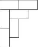
  Let

  $$\displaystyle \begin{aligned} F(x) = \sum_{n\geq 0}f(n)x^n = 1 + 2x +5x^2+10x^3+20x^4+ 36x^5+\cdots. \end{aligned}$$

  Show that

  $$\displaystyle \begin{aligned} F(x) = \prod_{n\geq 1}(1-x^n)^{-2}. \end{aligned}$$

• 8. (difficult) Let λ be a partition. Let m _k (λ) denote the number of parts of λ that are equal to k, and let η _k (λ) be the number of hooks of length k of λ. Show that

  $$\displaystyle \begin{aligned} \sum_{\lambda\vdash n}\eta_k(\lambda) = k\sum_{\lambda\vdash n} m_k(\lambda). \end{aligned}$$

• 9. (moderately difficult) Let μ be a partition, and let A _μ be the infinite shape consisting of the quadrant Q = {(i, j)  :  i < 0, j > 0} with the shape μ removed from the lower right-hand corner. Thus every square of A _μ has a finite hook and hence a hook length. For instance, when μ = (3, 1) we get the diagram

  

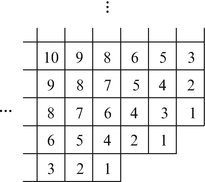
  Show that the multiset of hook lengths of A _μ is equal to the union of the multiset of hook lengths of Q (explicitly given by {1¹, 2², 3³, … }) and the multiset of hook lengths of μ.

• 10. In how many ways can we begin with the empty partition ∅, then add 2n squares one at a time (always keeping a partition), then remove n squares one at a time, then add n squares one at a time, and finally remove 2n squares one at a time, ending up at ∅?

• 11. (difficult) Fix n. Show that the number of partitions λ ⊢ n for which f ^λ is odd is equal to $2^{k_1+k_2+\dots }$, where k ₁ < k ₂ < ⋯ and $n=2^{k_1}+2^{k_2}+\cdots$ (the binary expansion of n). For instance, 75 = 2⁰ + 2¹ + 2³ + 2⁶, so the number of partitions λ of 75 for which f ^λ is odd is 2^6+3+1+0 = 1024.

• 12. Let U and D be the linear transformations associated with Young’s lattice. Write D ² U ² and D ³ U ³ in the form $\sum a_{ij}U^iD^j$.

• 13. Let U and D be the linear transformations associated with Young’s lattice. Suppose that f is some (noncommutative) polynomial in U and D satisfying f(U, D) = 0, e.g., f(U, D) = DU − UD − I. Let $i=\sqrt {-1}$. Show that f(iD, iU) = 0.

• 14. (*) Show that

  $$\displaystyle \begin{aligned} U^nD^n = (UD-(n-1)I)(UD-(n-2)I)\cdots (UD-I)UD, {}\end{aligned} $$

  (8.24)

  where U and D are the linear transformations associated with Young’s lattice (and I is the identity transformation), and where both sides of (8.24) operate on the vector space $\mathbb {R}Y_j$ (for some fixed j).

• 15. (difficult) Give a bijective proof of Corollary 8.8, i.e., β(2m, ∅) = 1 ⋅ 3 ⋅ 5⋯(2m − 1). Your proof should be an analogue of the RSK algorithm. To start with, note that [why?] 1 ⋅ 3 ⋅ 5⋯(2m − 1) is the number of complete matchings of [2m], i.e., the number of graphs on the vertex set [2m] with m edges such that every vertex is incident to exactly one edge.

• 16. Fix a partition λ ⊢ n − 1. Find a simple formula for the sum $t(\lambda ) = \sum _{\mu \gtrdot \lambda } f^\mu$ in terms of f ^λ. The sum ranges over all partitions μ that cover λ (i.e., μ > λ and nothing is in between, so μ ⊢ n) in Young’s lattice Y . Give a simple proof using linear algebra rather than a combinatorial proof.

• 17.

  • (a) (*) The Bell number B(n) is defined to be the number of partitions of an n-element set S, i.e., the number of sets {B ₁, …, B _k } where B _i  ≠ ∅, B _i  ∩ B _j  = ∅ if i ≠ j, and $\bigcup B_i=S$. Find a simple formula for the generating function

    $$\displaystyle \begin{aligned} F(x) =\sum_{n\geq 0} B(n)\frac{x^n}{n!} = 1+x+2\frac{x^2}{2!} +5\frac{x^3}{3!}+15\frac{x^4}{4!}+\cdots.\end{aligned} $$

  • (b) (moderately difficult) Let f(n) be the number of ways to move from the empty partition ∅ to ∅ in n steps, where each step consists of either (i) adding a box to the Young diagram, (ii) removing a box, or (iii) adding and then removing a box, always keeping the diagram of a partition (even in the middle of a step of type (iii)). For instance, f(3) = 5, corresponding to the five sequences

    $$\displaystyle \begin{aligned} \begin{array}{ccccc} \emptyset & (1,\emptyset) & (1,\emptyset) & (1,\emptyset)\\ \emptyset & (1,\emptyset) & 1 & \emptyset\\ \emptyset & 1 & (2,1) & \emptyset\\ \emptyset & 1 & (11,1) & \emptyset\\ \emptyset & 1 & \emptyset & (1,\emptyset) \end{array}. \end{aligned}$$

    Find (and prove) a formula for f(n) in terms of Bell numbers.

• 18. (difficult) (*) For n, k ≥ 0 let κ(n → n + k → n) denote the number of closed walks in Y  that start at level n, go up k steps to level n + k, and then go down k steps to level n. Thus for instance κ(n → n + 1 → n) is the number of cover relations between levels n and n + 1. Show that

  $$\displaystyle \begin{aligned} \sum_{n\geq 0}\kappa(n\to n+k\to n)q^n = k!\,(1-q)^{-k}F(Y,q). \end{aligned}$$

  Here F(Y, q) is the rank-generating function of Y , which by Proposition 8.14 (letting s →∞) is given by

  $$\displaystyle \begin{aligned} F(Y,q) = \prod_{i\geq 1}(1-q^i)^{-1}.\end{aligned} $$

• 19. Let X denote the formal sum of all elements of Young’s lattice Y . The operators U and D still act in the usual way on X, producing infinite linear combinations of elements of Y . For instance, the coefficient of the partition (3, 1) in DX is 3, coming from applying D to (4, 1), (3, 2), and (3, 1, 1).

  • (a) Show that DX = (U + I)X, where as usual I denotes the identity linear transformation.

  • (b) Express the coefficient s _n of ∅ (the empty partition) in D ⁿ X in terms of the numbers f ^λ for λ ⊢ n. (For instance, s ₀ = s ₁ = 1, s ₂ = 2, s ₃ = 4.)

  • (c) Show that

    $$\displaystyle \begin{aligned} D^{n+1}X = (UD^n+D^n+nD^{n-1})X,\ \ n\geq 0,\end{aligned} $$

    where D ⁻¹ = 0, D ⁰ = I.

  • (d) Find a simple recurrence relation satisfied by s _n .

  • (e) Find a simple formula for the generating function

    $$\displaystyle \begin{aligned} F(x)=\sum_{n\geq 0} s_n\frac{x^n}{n!}. \end{aligned}$$

  • (f) Show that s _n is the number of involutions in $\mathfrak {S}_n$, i.e., the number of elements $\pi \in \mathfrak {S}_n$ satisfying π ² = ι.

  • (g) (quite difficult) Show that if $\pi \in \mathfrak {S}_n$ and $\pi \stackrel {\mathrm {RSK}}{\longrightarrow } (P,Q)$, then $\pi ^{-1}\stackrel {\mathrm {RSK}}{\longrightarrow } (Q,P)$.

  • (h) Deduce your answer to (f) from (g).

• 20.

  • (a) Consider the linear transformation $U_{n-1}D_n\colon \mathbb {R} Y_n \to \mathbb {R} Y_n$. Show that its eigenvalues are the integers i with multiplicity p(n − i) − p(n − i − 1), for 0 ≤ i ≤ n − 2 and i = n.

  • (b) (*) Use (a) to give another proof of Theorem 8.9.

• 21.

  • (a) (moderately difficult) Let Y _[j−2,j] denote the Hasse diagram of the restriction of Young’s lattice Y  to the levels j − 2, j − 1, j. Let p(n) denote the number of partitions of n, and write Δp(n) = p(n) − p(n − 1). Show that the characteristic polynomial of the adjacency matrix of the graph Y _[j−2,j] is given by

    $$\displaystyle \begin{aligned} \pm x^{\Delta p(j)}(x^2-1)^{\Delta p(j-1)} \prod_{s=2}^j(x^3-(2s-1)x)^{\Delta p(j-1)}, \end{aligned}$$

    where the sign is $(-1)^{\#Y_{[j-2,j]}}=(-1)^{p(j-2)+p(j-1)+p(j)}$.

  • (b) (difficult) Extend to Y _[j−i,j] for any i ≥ 0. Express your answer in terms of the characteristic polynomial of matrices of the form

    $$\displaystyle \begin{aligned} \left[ \begin{array}{ccccccc} 0 & a & 0 & & & 0 & 0\\ 1 & 0 & a+1 & & & 0 & 0\\ 0 & 1 & 0 & & \ddots & 0 & 0\\ & & & \ddots\\ & & \ddots & & & 0 & b\\ & & & & & 1 & 0 \end{array} \right].\end{aligned} $$

• 22. (moderately difficult)

  • (a) Let U and D be operators (or just noncommutative variables) satisfying DU − UD = I. Show that for any power series $f(U)=\sum a_nU^n$ whose coefficients a _n are real numbers, we have

    $$\displaystyle \begin{aligned} e^{Dt}f(U) = f(U+t)e^{Dt}.\end{aligned} $$

    In particular,

    $$\displaystyle \begin{aligned} e^{Dt} e^{U} = e^{t+U}e^{Dt}. {} \end{aligned} $$

    (8.25)

    Here t is a variable (indeterminate) commuting with U and D. Regard both sides as power series in t whose coefficients are (noncommutative) polynomials in U and D. Thus for instance

    $$\displaystyle \begin{aligned} \begin{array}{rcl} e^{Dt}e^U &\displaystyle = &\displaystyle \left( \sum_{m\geq 0}\frac{D^nt^n}{n!} \right)\left( \sum_{n\geq 0}\frac{U^n}{n!}\right)\\ &\displaystyle = &\displaystyle \sum_{m,n\geq 0}\frac{D^mU^nt^m}{m!\,n!}. \end{array} \end{aligned} $$

  • (b) Show that $e^{(U+D)t} = e^{\frac 12 t^2+Ut}e^{Dt}$.

  • (c) Let δ _n be the total number of walks of length n in Young’s lattice Y  (i.e., in the Hasse diagram of Y ) starting at ∅. For instance, δ ₂ = 3 corresponding to the walks (∅, 1, 2), (∅, 1, 11), and (∅, 1, ∅). Find a simple formula for the generating function $F(t)=\sum _{n\geq 0}\delta _n\frac {t^n}{n!}$.

• 23. Let w be a balanced word in U and D, i.e., the same number of U’s as D’s. For instance, UUDUDDDU is balanced. Regard U and D as linear transformations on $\mathbb {R} Y$ in the usual way. A balanced word thus takes the space $\mathbb {R} Y_n$ to itself, where Y _n is the nth level of Young’s lattice Y . Show that the element $E_n = \sum _{\lambda \vdash n}f^\lambda \lambda \in \mathbb {R} Y_n$ is an eigenvector for w, and find the eigenvalue.

• 24. (*) Prove that any two balanced words (as defined in the previous exercise) commute.

• 25. Define a graded poset Z inductively as follows. The bottom level Z ₀ consists of a single element. Assume that we have constructed the poset up to level n. First “reflect” Z _n−1 through Z _n . More precisely, for each element x ∈ Z _n−1, let x′ be a new element of Z _n+1, with $x'\gtrdot y$ (where y ∈ Z _n ) if and only if $y\gtrdot x$. Then for each element y ∈ Z _n , let y′ be a new element of Z _n+1 covering y (and covering no other elements of Z _n ). Figure 8.1 shows the poset Z up to level 5. The cover relations obtained by the reflection construction are shown by solid lines, while those of the form $y'\gtrdot y$ are shown by broken lines.

  • (a) Show that #Z _n  = F _n+1 (a Fibonacci number), so the rank-generating function of Z is given by

    $$\displaystyle \begin{aligned} F(Z,q) = \frac{1}{1-q-q^2}. \end{aligned}$$

    Fig. 8.1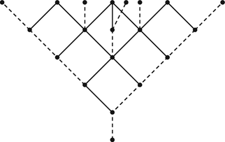

    

    The poset Z up to level 5

  • (b) Define $U_i\colon \mathbb {R} Z_i\to \mathbb {R} Z_{i+1}$ and $D_i\colon \mathbb {R} Z_i\to \mathbb {R} Z_{i-1}$ exactly as we did for Y , namely, for x ∈ Z _i we have

    $$\displaystyle \begin{aligned} \begin{array}{rcl} U_i(x) &\displaystyle = &\displaystyle \sum_{y\gtrdot x}y\\ D_i(x) &\displaystyle = &\displaystyle \sum_{y\lessdot x}y. \end{array} \end{aligned} $$

    Show that D _i+1 U _i  − U _i−1 D _i  = I _i . Thus all the results we have obtained for Y  based on this commutation relation also hold for Z! (For results involving p(n), we need only replace p(n) by F _n+1.)

• 26.

  • (a) Suppose that $\pi \in \mathfrak {S}_n$ and $\pi \stackrel {\mathrm {RSK}}{\longrightarrow } (P,Q)$. Let f(π) be the largest integer k for which 1, 2, …, k all appear in the first row of P. Find a simple formula for the number of permutations $\pi \in \mathfrak {S}_n$ for which f(π) = k.

  • (b) Let E(n) denote the expected value of f(π) for $\pi \in \mathfrak {S}_n$, i.e.,

    $$\displaystyle \begin{aligned} E(n) =\frac{1}{n!}\sum_{\pi\in\mathfrak{S}_n} f(\pi). \end{aligned}$$

    Find lim_n→∞ E(n).

• 27. Suppose that $\pi \in \mathfrak {S}_n$ and $\pi \stackrel {\mathrm {RSK}}{\longrightarrow } (P,Q)$. Let E ₁₂(n) be the expected value of the (1, 2)-entry of P (i.e., the second entry in the first row). Find lim_n→∞ E ₁₂(n).

• 28.

  • (a) An increasing subsequence of a permutation $a_1 a_2\cdots a_n\in \mathfrak {S}_n$ is a subsequence $a_{i_1}a_{i_2}\cdots a_{i_j}$ such that $a_{i_1}<a_{i_2}<\cdots <a_{i_j}$. For instance, 2367 is an increasing subsequence of the permutation 52386417. Suppose that the permutation $w\in \mathfrak {S}_n$ is sent into an SYT of shape λ = (λ ₁, λ ₂, … ) under the RSK algorithm. Show that λ ₁ is the length of the longest increasing subsequence of w.

  • (b) (much harder) Define decreasing subsequence similarly to increasing subsequence. Show that $\lambda ^{\prime }_1$ (the number of parts of λ) is equal to the length of the longest decreasing subsequence of λ.

  • (c) Assuming (a) and (b), show that for m, n ≥ 1, a permutation $w\in \mathfrak {S}_{mn+1}$ has an increasing subsequence of length m + 1 or a decreasing subsequence of length n + 1.

  • (d) How many permutations $w\in \mathfrak {S}_{mn}$ have longest increasing subsequence of length m and longest decreasing subsequence of length n? (Use the hook length formula to obtain a simple explicit answer.)

• 29. Write down the 13 plane partitions of 4 and the 24 plane partitions of 5.

• 30. Prove the statement preceding Lemma 8.17 that in the bijection $A\stackrel {\mathrm {RSK}^{\prime }}{\longrightarrow } (P,Q)$, equal elements of Q are inserted from left to right.

• 31. Let A be the r × s matrix of all 1’s. Describe the plane partition π′(A).

• 32.

  • (a) Find the $\mathbb {N}$-matrix A for which

    $$\displaystyle \begin{aligned} \pi'(A) = \begin{array}{ccccc} 6 & 4 & 4 & 3 & 3\\ 5 & 3 & 3 & 2\\ 3 & 2 & 1 \end{array}. \end{aligned}$$

  • (b) What message is conveyed by the nonzero entries of A?

• 33. (*) Let f(n) denote the number of plane partitions π = (π _ij ) of n for which π ₂₂ = 0. Show that

  $$\displaystyle \begin{aligned} \sum_{n\geq 0} f(n)x^n = \frac{\sum_{n\geq 0} (-1)^n x^{\binom{n+1}{2}}}{\prod_{i\geq 1}(1-x^i)^2}. \end{aligned}$$
• 34.

  • (a) (quite difficult) Let A be an r × s $\mathbb {N}$-matrix, and let $A\stackrel {\mathrm {RSK}^{\prime }}{\longrightarrow } (P,Q)$. If A ^t denotes the transpose of A, then show that $A^t\stackrel {\mathrm {RSK}^{\prime }}{\longrightarrow } (Q,P)$.

    Note. This result is quite difficult to prove from first principles. If you can do Exercise 8.19(g), then the present exercise is a straightforward modification. In fact, it is possible to deduce the present exercise from Exercise 8.19(g).

  • (b) A plane partition π = (π _ij ) is symmetric if π _ij  = π _ji for all i and j. Let s _r (n) denote the number of symmetric plane partitions of n with at most r rows. Assuming (a), show that

    $$\displaystyle \begin{aligned} \sum_{n\geq 0}s_r(n)x^n = \prod_{i=1}^r \left(1-x^{2i-1}\right)^{-1} \cdot \prod_{1\leq i<j\leq r}\left(1-x^{2(i+j-1)}\right)^{-1}. \end{aligned}$$

  • (c) Let s(n) denote the total number of symmetric plane partitions of n. Let r →∞ in (b) to deduce that

    $$\displaystyle \begin{aligned} \sum_{n\geq 0}s(n)x^n=\prod_{i\geq 1}\frac{1} {(1-x^{2i-1})(1-x^{2i})^{\lfloor i/2\rfloor}}. \end{aligned}$$

  • (d) (very difficult; cannot be done using RSK) Let s _rt (n) denote the number of symmetric plane partitions of n with at most r rows and with largest part at most t. Show that

    $$\displaystyle \begin{aligned} \sum_{n\geq 0} s_{rt}(n)x^n = \prod_{1\leq i<j\leq r} \prod_{k=1}^t\frac{1-x^{(2-\delta_{ij})(i+j+k-1)}} {1-x^{(2-\delta_{ij})(i+j+k-2)}}. \end{aligned}$$

• 35. The trace of a plane partition π = (π _ij ) is defined as tr(π) =∑ _i π _ii . Let pp(n, k) denote the number of plane partitions of n with trace k. Show that

  $$\displaystyle \begin{aligned} \sum_{n\geq 0}\sum_{k\geq 0}\mathrm{pp}(n,k)q^kx^n = \prod_{i\geq 1} (1-qx^i)^{-i}. \end{aligned}$$

• 36. (very difficult; cannot be done using RSK) Let pp _rst (n) be the number of plane partitions of n with at most r rows, at most s columns, and with largest part at most t. Show that

  $$\displaystyle \begin{aligned} \sum_{n\geq 0} \mathrm{pp}_{rst}(n)x^n = \prod_{i=1}^r\prod_{j=1}^s \prod_{k=1}^t \frac{1-x^{i+j+k-1}}{1-x^{i+j+k-2}}. \end{aligned}$$

• 37. Let f(n) denote the number of solid partitions of n with largest part at most 1. Find the generating function F(x) =∑_n≥0 f(n)x ⁿ.

References

E.A. Beem, Craige and Irene Schensted don’t have a car in the world, in Maine Times (March 12, 1982), pp. 20–21
E.A. Bender, D.E. Knuth, Enumeration of plane partitions. J. Comb. Theor. 13, 40–54 (1972)
S. Fomin, Duality of graded graphs. J. Algebr. Combin. 3, 357–404 (1994)
S. Fomin, Schensted algorithms for dual graded graphs. J. Algebr. Combin. 4, 5–45 (1995)
J.S. Frame, G. de B. Robinson, R.M. Thrall, The hook graphs of S n . Can. J. Math. 6 316–324 (1954)
D.S. Franzblau, D. Zeilberger, A bijective proof of the hook-length formula. J. Algorithms 3, 317–343 (1982)
F.G. Frobenius, Über die Charaktere der symmetrischen Gruppe, Sitzungsber. Kön. Preuss. Akad. Wissen. Berlin (1900), pp. 516–534; Gesammelte Abh. III, ed. by J.-P. Serre (Springer, Berlin, 1968), pp. 148–166
W.E. Fulton, Young Tableaux. Student Texts, vol. 35 (London Mathematical Society/Cambridge University Press, Cambridge, 1997)
C. Greene, A. Nijenhuis, H.S. Wilf, A probabilistic proof of a formula for the number of Young tableaux of a given shape. Adv. Math. 31, 104–109 (1979)
A.P. Hillman, R.M. Grassl, Reverse plane partitions and tableaux hook numbers. J. Comb. Theor. A 21, 216–221 (1976)
C. Krattenthaler, Bijective proofs of the hook formulas for the number of standard Young tableaux, ordinary and shifted. Electronic J. Combin. 2, R13, 9 pp. (1995)
D.E. Knuth, Permutations, matrices, and generalized Young tableaux. Pac. J. Math. 34, 709–727 (1970)
P.A. MacMahon, Memoir on the theory of the partitions of numbers — Part I. Philos. Trans. R. Soc. Lond. A 187, 619–673 (1897); Collected Works, vol. 1, ed. by G.E. Andrews (MIT, Cambridge, 1978), pp. 1026–1080
P.A. MacMahon, Memoir on the theory of the partitions of numbers — Part IV. Philos. Trans. R. Soc. Lond. A 209, 153–175 (1909); Collected Works, vol. 1, ed. by G.E. Andrews (MIT, Cambridge, 1978), pp. 1292–1314
P.A. MacMahon, Combinatory Analysis, vols. 1, 2 (Cambridge University Press, Cambridge, 1915/1916); Reprinted in one volume by Chelsea, New York, 1960
J.-C. Novelli, I. Pak, A.V. Stoyanovskii, A new proof of the hook-length formula. Discrete Math. Theor. Comput. Sci. 1, 053–067 (1997)
J.B. Remmel, Bijective proofs of formulae for the number of standard Young tableaux. Linear Multilinear Algebra 11, 45–100 (1982)
G. de B. Robinson, On the representations of S n . Am. J. Math. 60, 745–760 (1938)
B.E. Sagan, The Symmetric Group, 2nd edn. (Springer, New York, 2001)
C.E. Schensted, Longest increasing and decreasing subsequences. Can. J. Math. 13, 179–191 (1961)
R. Stanley, Differential posets. J. Am. Math. Soc. 1, 919–961 (1988)
R. Stanley, Variations on differential posets, in Invariant Theory and Tableaux, ed. by D. Stanton. The IMA Volumes in Mathematics and Its Applications, vol. 19 (Springer, New York, 1990), pp. 145–165
R. Stanley, Enumerative Combinatorics, vol. 1, 2nd edn. (Cambridge University Press, Cambridge, 2012)
R. Stanley, Enumerative Combinatorics, vol. 2 (Cambridge University Press, New York, 1999)
M.A.A. van Leeuwen, The Robinson-Schensted and Schützenberger algorithms, Part 1: new combinatorial proofs, Preprint no. AM-R9208 1992, Centrum voor Wiskunde en Informatica, 1992
A. Young, Qualitative substitutional analysis (third paper). Proc. Lond. Math. Soc. (2) 28, 255–292 (1927)
Author information
Authors and Affiliations
Rights and permissions
Copyright information
© 2018 Springer International Publishing AG, part of Springer Nature
About this chapter
Cite this chapter
Stanley, R.P. (2018). A Glimpse of Young Tableaux. In: Algebraic Combinatorics. Undergraduate Texts in Mathematics. Springer, Cham. https://doi.org/10.1007/978-3-319-77173-1_8
Download citation
DOI: https://doi.org/10.1007/978-3-319-77173-1_8
Published:
Publisher Name: Springer, Cham
Print ISBN: 978-3-319-77172-4
Online ISBN: 978-3-319-77173-1
eBook Packages: Mathematics and StatisticsMathematics and Statistics (R0)