Adaptive Oblivious Transfer with Access Control from Lattice Assumptions

Abstract

Adaptive oblivious transfer (OT) is a protocol where a sender initially commits to a database $\{M_i\}_{i=1}^N$. Then, a receiver can query the sender up to k times with private indexes $\rho _1,\ldots ,\rho _k$ so as to obtain $M_{\rho _1},\ldots , M_{\rho _k}$ and nothing else. Moreover, for each $i \in [k]$, the receiver’s choice $\rho _i$ may depend on previously obtained messages $\{M_{\rho _j}\}_{j <i}$. Oblivious transfer with access control (OT-AC) is a flavor of adaptive OT where database records are protected by distinct access control policies that specify which credentials a receiver should obtain in order to access each $M_i$. So far, all known OT-AC protocols only support access policies made of conjunctions or rely on ad hoc assumptions in pairing-friendly groups (or both). In this paper, we provide an OT-AC protocol where access policies may consist of any branching program of polynomial length, which is sufficient to realize any access policy in $\mathsf {NC1}$. The security of our protocol is proved under the Learning-with-Errors ($\mathsf {LWE}$) and Short-Integer-Solution ($\mathsf {SIS}$) assumptions. As a result of independent interest, we provide protocols for proving the correct evaluation of a committed branching program on a committed input.

1 Introduction

Oblivious transfer (OT) is a central cryptographic primitive coined by Rabin [45] and extended by Even et al. [20]. It involves a sender $\mathsf {S}$ with a database of messages $M_1, \ldots , M_N$ and a receiver $\mathsf {R}$ with an index $\rho \in \{1,\ldots ,N\}$. The protocol allows $\mathsf {R}$ to retrieve the $\rho$-th entry $M_{\rho }$ from $\mathsf {S}$ without letting $\mathsf {S}$ infer anything on $\mathsf {R}$’s choice $\rho$. Moreover, $\mathsf {R}$ only obtains $M_{\rho }$ learns nothing about $\{M_i\}_{i \ne \rho }$.

In its adaptive flavor [40], OT allows the receiver to interact k times with $\mathsf {S}$ to retrieve $M_{\rho _1},\ldots ,M_{\rho _k}$ in such a way that, for each $i \in \{2,\ldots ,k\}$, the i-th index $\rho _{i}$ may depend on the messages $M_{\rho _1},\ldots ,M_{\rho _{i-1}}$ previously obtained by $\mathsf {R}$.

OT is known to be a complete building block for cryptography (see, e.g., [24]) in that, if it can be realized, then any secure multiparty computation can be. In its adaptive variant, OT is motivated by applications in privacy-preserving access to sensitive databases (e.g., medical records or financial data) stored in encrypted form on remote servers, oblivious searches or location-based services.

As far as efficiency goes, adaptive OT protocols should be designed in such a way that, after an inevitable initialization phase with linear communication complexity in N and the security parameter $\lambda$, the complexity of each transfer is at most poly-logarithmic in N. At the same time, this asymptotic efficiency should not come at the expense of sacrificing ideal security properties. The most efficient adaptive OT protocols that satisfy the latter criterion stem from the work of Camenisch et al. [13] and its follow-ups [26,27,28].

In its basic form, (adaptive) OT does not restrict in any way the population of users who can obtain specific records. In many sensitive databases (e.g., DNA databases or patients’ medical history), however, not all users should be able to download all records: it is vital access to certain entries be conditioned on the receiver holding suitable credentials delivered by authorities. At the same time, privacy protection mandates that authorized users be able to query database records while leaking as little as possible about their interests or activities. In medical datasets, for example, the specific entries retrieved by a given doctor could reveal which disease his patients are suffering from. In financial or patent datasets, the access pattern of a company could betray its investment strategy or the invention it is developing. In order to combine user-privacy and fine-grained database security, it is thus desirable to enrich adaptive OT protocols with refined access control mechanisms in many of their natural use cases.

This motivated Camenisch et al. [11] to introduce a variant named oblivious transfer with access control (OT-AC), where each database record is protected by a different access control policy $P : \{0,1\}^*\rightarrow \{0,1\}$. Based on their attributes, users can obtain credentials generated by pre-determined authorities, which entitle them to anonymously retrieve database records of which the access policy accepts their certified attributes: in other words, the user can only download the records for which he has a valid credential $\mathsf {Cred}_x$ for an attribute string $x \in \{0,1\}^*$ such that $P(x)=1$. During the transfer phase, the user demonstrates possession of a pair $(\mathsf {Cred}_x,x)$ and simultaneously convinces the sender that he is querying some record $M_{\rho }$ associated with a policy P such that $P(x)=1$. The only information that the database holder eventually learns is that some user retrieved some record which he was authorized to obtain.

Camenisch et al. formalized the OT-AC primitive and provided a construction in groups with a bilinear map [11]. While efficient, their solution “only” supports access policies consisting of conjunctions: each policy P is specified by a list of attributes that a given user should obtain a credential for in order to complete the transfer. Several subsequent works [10, 12, 50] considered more expressive access policies while even hiding the access policies in some cases [10, 12]. Unfortunately, all of them rely on non-standard assumptions (known as “q-type assumptions”) in groups with a bilinear maps. For the sake of not putting all one’s eggs in the same basket, a primitive as powerful as OT-AC ought to have alternative realizations based on firmer foundations.

In this paper, we propose a solution based on lattice assumptions where access policies consist of any branching program of width 5, which is known [6] to suffice for the realization of any access policy in $\mathsf {NC1}$. As a result of independent interest, we provide protocols for proving the correct evaluation of a committed branching program. More precisely, we give zero-knowledge arguments for demonstrating possession of a secret input $\mathbf x \in \{0,1\}^\kappa$ and a secret (and possibly certified) branching program $\mathsf {BP}$ such that $\mathsf {BP}(\mathbf x)=1$.

Related Work. Oblivious transfer with adaptive queries dates back to the work of Naor and Pinkas [40], which requires $O( \log N)$ interaction rounds per transfer. Naor and Pinkas [42] also gave generic constructions of (adaptive) k-out-of-N OT from private information retrieval (PIR) [16]. The constructions of [40, 42], however, are only secure in the half-simulation model, where simulation-based security is only considered for one of the two parties (receiver security being formalized in terms of a game-based definition). Moreover, the constructions of Adaptive OT from PIR [42] require a complexity $O(N^{1/2})$ at each transfer where Adaptive OT allows for $O(\log N)$ cost. Before 2007, many OT protocols (e.g., [3, 41, 49]) were analyzed in terms of half-simulation.

While several efficient fully simulatable protocols appeared the last 15 years (e.g., [37, 44] and references therein), full simulatability remained elusive in the adaptive k-out-of-N setting [40] until the work [13] of Camenisch, Neven and shelat, who introduced the “assisted decryption” paradigm. The latter consists in having the sender obliviously decrypt a re-randomized version of one of the original ciphertexts contained in the database. This technique served as a blueprint for many subsequent protocols [26,27,28, 31], including those with access control [1, 10,11,12] and those presented in this paper. In the adaptive k-out-of-N setting (which we denote as $\mathcal {OT}_{k \times 1}^N$), the difficulty is to achieve full simulatability without having to transmit a O(N) bits at each transfer. To our knowledge, except the oblivious-PRF-based approach of Jarecki and Liu [31], all known fully simulatable $\mathcal {OT}_{k \times 1}^N$ protocols rely on bilinear maps.¹

A number of works introduced various forms of access control in OT. Priced OT [3] assigns variable prices to all database records. In conditional OT [18], access to a record is made contingent on the user’s secret satisfying some predicate. Restricted OT [29] explicitly protects each record with an independent access policy. Still, none of these OT flavors aims at protecting the anonymity of users. The model of Coull et al. [17] does consider user anonymity via stateful credentials. For the applications of OT-AC, it would nevertheless require re-issuing user credentials at each transfer.

While efficient, the initial OT-AC protocol of Camenisch et al. [11] relies on non-standard assumptions in groups with a bilinear map and only realizes access policies made of conjunctions. Abe et al. [1] gave a different protocol which they proved secure under more standard assumptions in the universal composability framework [14]. Their policies, however, remain limited to conjunctions. It was mentioned in [1, 11] that disjunctions and DNF formulas can be handled by duplicating database entries. Unfortunately, this approach rapidly becomes prohibitively expensive in the case of (t, n)-threshold policies with $t \approx n/2$. Moreover, securing the protocol against malicious senders requires them to prove that all duplicates encrypt the same message. More expressive policies were considered by Zhang et al. [50] who gave a construction based on attribute-based encryption [47] that extends to access policies expressed by any Boolean formulas (and thus $\mathsf {NC}1$ circuits). Camenisch et al. [12] generalized the OT-AC functionality so as to hide the access policies. In [10], Camenisch et al. gave a more efficient construction with hidden policies based on the attribute-based encryption scheme of [43]. At the expense of a proof in the generic group model, [10] improves upon the expressiveness of [12] in that its policies extend into CNF formulas. While the solutions of [10, 12] both hide the access policies to users (and the successful termination of transfers to the database), their policies can only live in a proper subset of $\mathsf {NC1}$. As of now, threshold policies can only be efficiently handled by the ABE-based construction of Zhang et al. [50], which requires ad hoc assumptions in groups with a bilinear map.

Our Results and Techniques. We describe the first OT-AC protocol based on lattice assumptions. Our construction supports access policies consisting of any branching program of width 5 and polynomial length – which suffices to realize any $\mathsf {NC1}$ circuit – and prove it secure under the $\mathsf {SIS}$ and $\mathsf {LWE}$ assumptions. We thus achieve the same level of expressiveness as [50] with the benefit of relying on well-studied assumptions. In its initial version, our protocol requires the database holder to communicate $\varTheta (N)$ bits to each receiver so as to prove that the database is properly encrypted. In the random oracle model, we can eliminate this burden via the Fiat-Shamir heuristic and make the initialization cost linear in the database size N, regardless of the number of users.

As a first step, we build an ordinary $\mathcal {OT}_{k \times 1}^N$ protocol (i.e., without access control) via the “assisted decryption” approach of [13]. In short, the sender encrypts all database entries using a semantically secure cryptosystem. At each transfer, the receiver gets the sender to obliviously decrypt one of the initial ciphertexts without learning which one. Security against malicious adversaries is achieved by adding zero-knowledge (ZK) or witness indistinguishable (WI) arguments that the protocol is being followed. The desired ZK or WI arguments are obtained using the techniques of [34] and we prove that this basic protocol satisfies the full imulatability definitions of [13] under the $\mathsf {SIS}$ and $\mathsf {LWE}$ assumptions. To our knowledge, this protocol is also the first $\mathcal {OT}_{k \times 1}^N$ realization to achieve the standard simulation-based security requirements under lattice assumptions.

So far, all known “beyond-conjunctions” OT-AC protocols [10, 50] rely on ciphertext-policy attribute-based encryption (CP-ABE) and proceed by attaching each database record to a CP-ABE ciphertext. Our construction departs from the latter approach for two reasons. First, the only known $\mathsf {LWE}$-based CP-ABE schemes are obtained by applying a universal circuit to a key-policy system, making them very inefficient. Second, the ABE-based approach requires a fully secure ABE (i.e., selective security and semi-adaptive security are insufficient) since the access policies are dictated by the environment after the generation of the issuer’s public key, which contains the public parameters of the underlying ABE in [10, 50]. Even with the best known $\mathsf {LWE}$-based ABE candidates [25], a direct adaptation of the techniques in [10, 50] would incur to rely on a complexity leveraging argument [8] and a universal circuit. Instead, we take a different approach and directly prove in a zero-knowledge manner the correct evaluation of a committed branching program for a hidden input.

At a high level, our OT-AC protocol works as follows. For each $i \in [N]$, the database entry $M_i \in \{0,1\}^t$ is associated with branching program $\mathsf {BP}_i$. In the initialization step, the database holder generates a Regev ciphertext $(\mathbf {a}_i, \mathbf {b}_i)$ of $M_i$, and issues a certificate for the pair $\big ((\mathbf {a}_i, \mathbf {b}_i), \mathsf {BP}_i\big )$, using the signature scheme from [34]. At each transfer, the user $\mathsf {U}$ who wishes to get a record $\rho \in [N]$ must obtain a credential $\mathsf {Cred}_{\mathbf {x}}$ for an attribute string $\mathbf {x} \in \{0,1\}^\kappa$ such that $\mathsf {BP}_{\rho }(\mathbf {x})=1$. Then, $\mathsf {U}$ modifies $(\mathbf {a}_{\rho },\mathbf {b}_{\rho })$ into an encryption of $M_\rho \oplus \mu \in \{0,1\}^t$, for some random string $\mu \in \{0,1\}^t$, and re-randomizes the resulting ciphertext into a fresh encryption $(\mathbf {c}_0,\mathbf {c}_1)$ of $M_{\rho } \oplus \mu$. At this point, $\mathsf {U}$ proves that $(\mathbf {c}_0,\mathbf {c}_1)$ was obtained by transforming one of the original ciphertexts $\{(\mathbf {a}_i,\mathbf {b}_i)\}_{i=1}^N$ by arguing possession of a valid certificate for $\big ((\mathbf {a}_{\rho }, \mathbf {b}_{\rho }), \mathsf {BP}_{\rho }\big )$ and knowledge of all randomness used in the transformation that yields $(\mathbf {c}_0,\mathbf {c}_1)$. At the same time, $\mathsf {U}$ proves possession of $\mathsf {Cred}_{\mathbf {x}}$ for a string $\mathbf {x}$ which is accepted by the committed $\mathsf {BP}_{\rho }$. To demonstrate these statements in zero-knowledge, we develop recent techniques [34, 36, 39] for lattice-based analogues [32, 38] of Stern’s protocol [48].

As a crucial component of our OT-AC protocol, we need to prove knowledge of an input $\mathbf {x} = (x_0, \ldots , x_{\kappa -1})^\top \in \{0,1\}^\kappa$ satisfying a hidden $\mathsf {BP}$ of length L, where L and $\kappa$ are polynomials in the security parameter. For each $\theta \in [L]$, we need to prove that the computation of the $\theta$-th state

$$\begin{aligned} \eta _\theta = \pi _{\theta , 0}(\eta _{\theta -1})\cdot (1-x_{\mathrm {var}(\theta )}) + \pi _{\theta , 1}(\eta _{\theta -1})\cdot {x}_{\mathrm {var}(\theta )}, \end{aligned}$$

(1)

is done correctly, for permutations $\pi _{\theta , 0}, \pi _{\theta , 1}: [0,4] \rightarrow [0,4]$ and for integer $\mathrm {var}(\theta ) \in [0,\kappa -1]$ specified by $\mathsf {BP}$. To date, equations of the form (1) have not been addressed in the context of zero-knowledge proofs for lattice-based cryptography. In this work, we are not only able to handle L such equations, but also manage to do so with a reasonable asymptotic cost.

In order to compute $\eta _{\theta }$ as in (1), we have to fetch the value $x_{\mathrm {var}(\theta )}$ in the input $(x_0, \ldots , x_{\kappa -1})^\top$ and provide evidence that the searching process is conducted honestly. If we perform a naive left-to-right search in the array $x_0, \ldots , x_{\kappa -1}$, the expected complexity is $\mathcal {O}(\kappa )$ for each step, and the total complexity amounts to $\mathcal {O}(L \cdot \kappa )$. If we instead perform a dichotomic search over $x_0, \ldots , x_{\kappa -1}$, we can decrease the complexity at each step down to $\mathcal {O}(\log \kappa )$. However, in this case, we need to prove in zero-knowledge a statement “I obtained $x_{\mathrm {var}(\theta )}$ by conducting a correct dichotomic search in my secret array.”

We solve this problem as follows. For each $i \in [0,\kappa -1]$, we employ a SIS-based commitment scheme [32] to commit to $x_i$ as $\mathsf {com}_i$, and prove that the committed bits are consistent with the ones involved in the credential $\mathsf {Cred}_{\mathbf {x}}$ mentioned above. Then we build a SIS-based Merkle hash tree [36] of depth $\delta _\kappa = \lceil \log \kappa \rceil$ on top of the commitments $\mathsf {com}_0, \ldots , \mathsf {com}_{\kappa -1}$. Now, for each $\theta \in [L]$, we consider the binary representation $d_{\theta , 1}, \ldots , d_{\theta , \delta _\kappa }$ of $\mathrm {var}(\theta )$. We then prove knowledge of a bit $y_\theta$ such that these conditions hold: “If one starts at the root of the tree and follows the path determined by the bits $d_{\theta , 1}, \ldots , d_{\theta , \delta _\kappa }$, then one will reach the leaf associated with the commitment opened to $y_\theta$.” The idea is that, if the Merkle tree and the commitment scheme are both secure, then it should be true that $y_\theta = x_{\mathrm {var}(\theta )}$. In other words, this enables us to provably perform a “binary search” for $x_{\mathrm {var}(\theta )} = y_\theta$. Furthermore, this process can be done in zero-knowledge, by adapting the recent techniques from [36]. As a result, we obtain a protocol with communication cost just $\mathcal {O}(L \cdot \log \kappa + \kappa )$.

2 Background and Definitions

Vectors are denoted in bold lower-case letters and bold upper-case letters will denote matrices. The Euclidean and infinity norm of any vector $\mathbf {b} \in \mathbb R^n$ will be denoted by $\Vert \mathbf {b}\Vert$ and $\Vert \mathbf {b}\Vert _\infty$, respectively. The Euclidean norm of matrix $\mathbf {B} \in \mathbb R^{m \times n}$ with columns $(\mathbf {b}_i)_{i \le n}$ is $\Vert \mathbf {B}\Vert = \max _{i\le n} \Vert \mathbf {b}_i\Vert$. When $\mathbf {B}$ has full column-rank, we let $\widetilde{\mathbf {B}}$ denote its Gram-Schmidt orthogonalization.

When S is a finite set, we denote by U(S) the uniform distribution over S, and by $x \hookleftarrow U(S)$ the action of sampling x according to this distribution. Finally for any integers A, B, N, we let [N] and [A, B] denote the sets $\{1, \ldots , N\}$ and $\{A,A+1,\ldots ,B\}$, respectively.

2.1 Lattices

A lattice L is the set of integer linear combinations of linearly independent basis vectors $(\mathbf {b}_i)_{i\le n}$ living in $\mathbb R^m$. We work with q-ary lattices, for some prime q.

Definition 1

Let $m \ge n \ge 1$, a prime $q \ge 2$ and $\mathbf {A} \in \mathbb {Z}_q^{n \times m}$ and $\mathbf {u} \in \mathbb {Z}_q^n$, define $\varLambda _q(\mathbf {A}) := \{ \mathbf {e} \in \mathbb {Z}^m \mid \exists \mathbf {s} \in \mathbb {Z}_q^n~\text {s.t.}~\mathbf {A}^T \cdot \mathbf {s} = \mathbf {e} \bmod q \}$ as well as

$$\begin{aligned} \varLambda _q^{\perp } (\mathbf {A}) := \{\mathbf {e} \in \mathbb {Z}^m \mid \mathbf {A} \cdot \mathbf {e} = \mathbf {0}^n \bmod q \},\, \varLambda _q^{\mathbf {u}} (\mathbf {A}) := \{\mathbf {e} \in \mathbb {Z}^m \mid \mathbf {A} \cdot \mathbf {e} = \mathbf {u} \bmod q \}. \end{aligned}$$

For a lattice L, let $\rho _{\sigma ,\mathbf {c}}(\mathbf {x}) = \exp (-\pi \Vert \mathbf {x}- \mathbf {c} \Vert ^2/\sigma ^2)$ for a vector $\mathbf {c} \in \mathbb R^m$ and a real $\sigma >0$. The discrete Gaussian of support L, center $\mathbf {c}$ and parameter $\sigma$ is $D_{L,\sigma ,\mathbf {c}}(\mathbf {y}) = \rho _{\sigma ,\mathbf {c}}(\mathbf {y})/\rho _{\sigma ,\mathbf {c}}(L)$ for any $\mathbf {y} \in L$, where $\rho _{\sigma ,\mathbf {c}}(L) =\sum _{\mathbf {x} \in L} \rho _{\sigma ,\mathbf {c}}(\mathbf {x})$. The distribution centered in $\mathbf {c}=\mathbf {0}$ is denoted by $D_{L,\sigma }(\mathbf {y})$.

It is well known that one can efficiently sample from a Gaussian distribution with lattice support given a sufficiently short basis of the lattice.

Lemma 1

[9, Lemma 2.3]. There exists a PPT algorithm $\mathsf {GPVSample}$ that takes as inputs a basis $\mathbf {B}$ of a lattice $L \subseteq \mathbb {Z}^n$ and a rational $\sigma \ge \Vert \widetilde{\mathbf {B}}\Vert \cdot \varOmega (\sqrt{\log n})$, and outputs vectors $\mathbf {b} \in L$ with distribution $D_{L,\sigma }$.

We also rely on the trapdoor generation algorithm of Alwen and Peikert [4], which refines the technique of Gentry et al. [22].

Lemma 2

[4, Theorem 3.2]. There is a PPT algorithm $\mathsf {TrapGen}$ that takes as inputs $1^n$, $1^m$ and an integer $q \ge 2$ with $m \ge \varOmega (n \log q)$, and outputs a matrix $\mathbf {A} \in \mathbb {Z}_q^{n \times m}$ and a basis $\mathbf {T}_{\mathbf {A}}$ of $\varLambda _q^{\perp }(\mathbf {A})$ such that $\mathbf {A}$ is within statistical distance $2^{-\varOmega (n)}$ to $U(\mathbb {Z}_q^{n \times m})$, and $\Vert \widetilde{\mathbf {T}_{\mathbf {A}}}\Vert \le \mathcal {O}(\sqrt{n \log q})$.

We use the basis delegation algorithm [15] that inputs a trapdoor for $\mathbf {A} \in \mathbb {Z}_q^{n \times m}$ and produces a trapdoor for any $\mathbf {B} \in \mathbb {Z}_q^{n \times m'}$ containing $\mathbf {A}$ as a submatrix. A technique from Agrawal et al. [2] is sometimes used in our proofs.

Lemma 3

[15, Lemma 3.2]. There is a PPT algorithm $\mathsf {ExtBasis}$ that inputs $\mathbf {B} \in \mathbb {Z}_q^{n \times m' }$ whose first m columns span $\mathbb {Z}_q^n$, and a basis $\mathbf {T}_{\mathbf {A}}$ of $\varLambda _q^{\perp }(\mathbf {A})$ where $\mathbf {A} \in \mathbb {Z}_q^{n \times m}$ is a submatrix of $\mathbf {B}$, and outputs a basis $\mathbf {T}_{\mathbf {B}}$ of $\varLambda _q^{\perp }(\mathbf {B})$ with $\Vert \widetilde{\mathbf {T}_{\mathbf {B}}}\Vert \le \Vert \widetilde{\mathbf {T}_{\mathbf {A}}}\Vert$.

Lemma 4

[2, Theorem 19]. There is a PPT algorithm $\mathsf {SampleRight}$ that inputs $\mathbf A, \mathbf C \in \mathbb {Z}_q^{n \times m}$, a small-norm $\mathbf R \in \mathbb {Z}^{m \times m}$, a short basis $\mathbf {T_C} \in \mathbb {Z}^{m \times m}$ of $\varLambda _q^{\perp }(\mathbf {C})$, a vector $\mathbf u \in \mathbb {Z}_q^{n}$ and a rational $\sigma$ such that $\sigma \ge \Vert \widetilde{\mathbf {T_C}}\Vert \cdot \varOmega (\sqrt{\log n})$, and outputs $\mathbf {b} \in \mathbb {Z}^{2m}$ such that $\left[ \begin{array}{c|c} \mathbf A~&~\mathbf A \cdot \mathbf R + \mathbf C \end{array} \right] \cdot \mathbf b = \mathbf u \bmod q$ and with distribution statistically close to $D_{L,\sigma }$ where $L=\{ {\mathbf x} \in \mathbb {Z}^{2 m} : \left[ \begin{array}{c|c} {\mathbf A} ~&~ {\mathbf A} \cdot {\mathbf R} + {\mathbf C} \end{array} \right] \cdot \mathbf x = \mathbf u \bmod q \}$.

2.2 Hardness Assumptions

Definition 2

Let $n,m,q,\beta$ be functions of $\lambda \in \mathbb {N}$. The Short Integer Solution problem $\mathsf {SIS}_{n,m,q,\beta }$ is, given $\mathbf {A} \hookleftarrow U(\mathbb {Z}_q^{n \times m})$, find $\mathbf {x} \in \varLambda _q^{\perp }(\mathbf {A})$ with $0 < \Vert \mathbf {x}\Vert \le \beta$.

If $q \ge \sqrt{n} \beta$ and $m,\beta \le \mathsf {poly}(n)$, then standard worst-case lattice problems with approximation factors $\gamma = \widetilde{\mathcal {O}}(\beta \sqrt{n})$ reduce to $\mathsf {SIS}_{n,m,q,\beta }$ (see, e.g., [22, Sect. 9]).

Definition 3

Let $n,m \ge 1$, $q \ge 2$, and let $\chi$ be a probability distribution on $\mathbb {Z}$. For $\mathbf {s} \in \mathbb {Z}_q^n$, let $A_{\mathbf {s}, \chi }$ be the distribution obtained by sampling $\mathbf {a} \hookleftarrow U(\mathbb {Z}_q^n)$ and $e \hookleftarrow \chi$, and outputting $(\mathbf {a}, \mathbf {a}^T\cdot \mathbf {s} + e) \in \mathbb {Z}_q^n \times \mathbb {Z}_q$. The Learning With Errors problem $\mathsf {LWE}_{n,q,\chi }$ asks to distinguish m samples chosen according to $\mathcal {A}_{\mathbf {s},\chi }$ (for $\mathbf {s} \hookleftarrow U(\mathbb {Z}_q^n)$) and m samples chosen according to $U(\mathbb {Z}_q^n \times \mathbb {Z}_q)$.

If q is a prime power, $B \ge \sqrt{n}\omega (\log n)$, $\gamma = \widetilde{\mathcal {O}}(nq/B)$, then there exists an efficient sampleable B-bounded distribution $\chi$ (i.e., $\chi$ outputs samples with norm at most B with overwhelming probability) such that $\mathsf {LWE}_{n,q,\chi }$ is as least as hard as $\mathsf {SIVP}_{\gamma }$ (see, e.g., [9, 46]).

2.3 Adaptive Oblivious Transfer

In the syntax of [13], an adaptive k-out-of-N OT scheme $\mathcal {OT} _k^N$ is a tuple of stateful $\mathsf {PPT}$ algorithms $(\mathsf {S_I}, \mathsf {R_I}, \mathsf {S_T}, \mathsf {R_T})$. The sender $\mathsf {S}=(\mathsf {S_I},\mathsf {S_T})$ consists of two interactive algorithms $\mathsf {S_I}$ and $\mathsf {S_T}$ and the receiver has a similar representation as algorithms $\mathsf {R_I}$ and $\mathsf {R_T}$. In the initialization phase, the sender and the receiver run interactive algorithms $\mathsf {S_I}$ and $\mathsf {R_I}$, respectively, where $\mathsf {S_I}$ takes as input messages $M_1, \ldots , M_N$ while $\mathsf {R_I}$ has no input. This phase ends with the two algorithms $\mathsf {S_I}$ and $\mathsf {R_I}$ outputting their state information $S_0$ and $R_0$ respectively.

During the i-th transfer, $1 \le i \le k$, both parties run an interactive protocol via the $\mathsf {R_T}$ and $\mathsf {S_T}$ algorithms. The sender starts runs $\mathsf {S_T} (S_{i-1})$ to obtain its updated state information $S_i$ while the receiver runs $\mathsf {R_T} (R_{i-1}, \rho _i)$ on input of its previous state $R_{i-1}$ and the index $\rho _i \in \{1, \ldots , N \}$ of the message it wishes to retrieve. At the end, $\mathsf {R_T}$ outputs an updated state $R_i$ and a message $M'_{\rho _i}$.

Correctness mandates that, for all $M_1, \ldots , M_N$, for all $\rho _1, \ldots , \rho _k \in [ N]$ and all coin tosses $\varpi$ of the (honestly run) algorithms, we have $M'_{\rho _i} = M_{\rho _i}$ for all i.

We consider protocols that are secure (against static corruptions) in the sense of simulation-based definitions. The security properties against a cheating sender and a cheating receiver are formalized via the “real-world/ideal-world” paradigm. The security definitions of [13] are recalled in the full paper.

2.4 Adaptive Oblivious Transfer with Access Control

Camenisch et al. [11] define oblivious transfer with access control (OT-AC) as a tuple of PPT algorithms/protocols $(\mathsf {ISetup}, \mathsf {Issue}, \mathsf {DBSetup}, \mathsf {Transfer})$ such that:

• ISetup : takes as inputs public parameters $\mathsf {pp}$ specifying a set $\mathcal {P}$ of access policies and generates a key pair $(PK_I, SK_I)$ for the issuer.

• Issue : is an interactive protocol between the issuer I and a stateful user $\mathsf {U}$ under common input $(\mathsf {pp}, {x})$, where x is an attribute string. The issuer I takes as inputs its key pair $(PK_I, SK_I)$ and a user pseudonym $P_\mathsf {U}$. The user takes as inputs its state information $st_\mathsf {U}$. The user $\mathsf {U}$ outputs either an error symbol $\bot$ or a credential $\mathsf {Cred}_\mathsf {U}$, and an updated state $st'_\mathsf {U}$.

• DBSetup : is an algorithm that takes as input the issuer’s public key $PK_I$, a database $DB = \left( M_i, \mathsf {AP}_i \right) _{i=1}^N$ containing records $M_i$ whose access is restricted by an access policy $\mathsf {AP}_i$ and outputs a database public key $PK_\mathrm {DB}$, an encryption of the records $(ER_i)_{i=1}^N$ and a database secret key $SK_\mathrm {DB}$.

• Transfer : is a protocol between the database $\mathsf {DB}$ and a user $\mathsf {U}$ with common inputs $(PK_I, PK_\mathrm {DB})$. $\mathsf {DB}$ inputs $SK_\mathrm {DB}$ and $\mathsf {U}$ inputs $(\rho , st_\mathsf {U}, ER_\rho , \mathsf {AP}_\rho )$, where $\rho \in [N]$ is a record index to which $\mathsf {U}$ is requesting access. The interaction ends with $\mathsf {U}$ outputting $\bot$ or a string $M_{\rho '}$ and an updated state $st'_\mathsf {U}$.

We assume private communication links, so that communications between a user and the issuer are authenticated, and those between a user and the database are anonymized: otherwise, anonymizing the $\mathsf {Transfer}$ protocol is impossible.

The security definitions formalize two properties called user anonymity and database security. The former captures that the database should be unable to tell which honest user is making a query and neither can tell which records are being accessed. This should remain true even if the database colludes with corrupted users and the issuer. As for database security, the intuition is that a cheating user cannot access a record for which it does not have the required credentials, even when colluding with other dishonest users. In case the issuer is colluding with these cheating users, they cannot obtain more records from the database than they retrieve. Precise security definitions [11] are recalled in the full version of the paper.

2.5 Vector Decompositions

We will employ the decomposition technique from [34, 38], which allows transforming vectors with infinity norm larger than 1 into vectors with infinity norm 1.

For any $B \in \mathbb {Z}_+$, define the number $\delta _B:=\lfloor \log _2 B\rfloor +1 = \lceil \log _2(B+1)\rceil$ and the sequence $B_1, \ldots , B_{\delta _B}$, where $B_j = \lfloor \frac{B + 2^{j-1}}{2^j} \rfloor$, $\forall j \in [1,\delta _B]$. This sequence satisfies $\sum _{j=1}^{\delta _B} B_j = B$ and any integer $v \in [0, B]$ can be decomposed to $\mathsf {idec}_B(v) = (v^{(1)}, \ldots , v^{(\delta _B)})^\top \in \{0,1\}^{\delta _B}$ such that $\sum _{j=1}^{\delta _B}B_j \cdot v_j = v$. We describe this decomposition procedure in a deterministic manner as follows:

• 1. Set $v': = v$; For $j=1$ to $\delta _B$ do:

  • If $v' \ge B_j$ then $v^{(j)}: = 1$, else $v^{(j)}: = 0$; $v': = v' - B_j\cdot v^{(j)}$.

• 2. Output $\mathsf {idec}_B(v) = (v^{(1)}, \ldots , v^{(\delta _B)})^\top$.

For any positive integers $\mathfrak {m}, B$, we define $\mathbf {H}_{\mathfrak {m},B}: = \mathbf {I}_{\mathfrak {m}} \otimes [ B_1 | \ldots | B_{\delta _B} ] \in \mathbb {Z}^{\mathfrak {m} \times \mathfrak {m}\delta _B}$ and the following injective functions:

• (i) $\mathsf {vdec}_{\mathfrak {m}, B}: [0,B]^{\mathfrak {m}} \rightarrow \{0,1\}^{\mathfrak {m}\delta _B}$ that maps vector $\mathbf {v} = (v_1, \ldots , v_{\mathfrak {m}})$ to vector $\big (\mathsf {idec}_B(v_1)^\top \Vert \ldots \Vert \mathsf {idec}_B(v_{\mathfrak {m}})^\top \big )^\top$. Note that $\mathbf {H}_{\mathfrak {m}, B} \cdot \mathsf {vdec}_{\mathfrak {m}, B}(\mathbf {v}) = \mathbf {v}$.

• (ii) $\mathsf {vdec}'_{\mathfrak {m}, B}: [-B,B]^{\mathfrak {m}} \rightarrow \{-1,0,1\}^{\mathfrak {m}\delta _B}$ that maps vector $\mathbf {w} = (w_1, \ldots , w_{\mathfrak {m}})$ to vector $\big (\sigma (w_1)\cdot \mathsf {idec}_B(|w_1|)^\top \Vert \ldots \Vert \sigma (w_{\mathfrak {m}})\cdot \mathsf {idec}_B(|w_{\mathfrak {m}}|)^\top \big )^\top$, where for each $i=1, \ldots , \mathfrak {m}$: $\sigma (w_i) = 0$ if $w_i =0$; $\sigma (w_i) = -1$ if $w_i <0$; $\sigma (w_i) = 1$ if $w_i >0$. Note that $\mathbf {H}_{\mathfrak {m}, B} \cdot \mathsf {vdec}'_{\mathfrak {m}, B}(\mathbf {w}) = \mathbf {w}$.

3 Building Blocks

We will use two distinct signature schemes because one of them only needs to be secure in the sense of a weaker security notion and can be more efficient. This weaker notion is sufficient to sign the database entries and allows a better efficiency in the scheme of Sect. 4.

3.1 Signatures Supporting Efficient Zero-Knowledge Proofs

We use a signature scheme proposed by Libert et al. [34] who extended the Böhl et al. signature [7] in order to sign messages comprised of multiple blocks while keeping the scheme compatible with zero-knowledge proofs.

• Keygen $(1^\lambda ,1^{N_b})$ : Given a security parameter $\lambda >0$ and the number of blocks $N_b = \mathsf {poly}(\lambda )$, choose $n = \mathcal {O}(\lambda )$, a prime modulus $q = \widetilde{\mathcal {O}}(N\cdot n^{4})$, a dimension $m =2n \lceil \log q \rceil$; an integer $\ell = \mathsf {poly}(n)$ and Gaussian parameters $\sigma = \varOmega (\sqrt{n\log q}\log n)$. Define the message space as $\mathcal {M}=(\{0,1\}^{m_I})^{N_b}$.

  • 1. Run $\mathsf {TrapGen}(1^n,1^m,q)$ to get $\mathbf {A} \in \mathbb {Z}_q^{n \times m}$ and a short basis $\mathbf {T}_{\mathbf {A}}$ of $\varLambda _q^{\perp }(\mathbf {A}).$ This basis allows computing short vectors in $\varLambda _q^{\perp }(\mathbf {A})$ with a Gaussian parameter $\sigma$. Next, choose $\ell +1$ random $\mathbf {A}_0,\mathbf {A}_1,\ldots ,\mathbf {A}_{\ell } \hookleftarrow U(\mathbb {Z}_q^{n \times m})$.

  • 2. Choose random matrices $\mathbf {D} \hookleftarrow U(\mathbb {Z}_q^{n \times m/2})$, $\mathbf {D}_0 \hookleftarrow U(\mathbb {Z}_q^{n \times m}), \mathbf {D}_j \hookleftarrow U(\mathbb {Z}_q^{n \times m_I})$ for $j=1,\ldots ,N_b$, as well as a random vector $\mathbf {u} \hookleftarrow U(\mathbb {Z}_q^n)$.

  The private signing key consists of $SK:= \mathbf {T}_{\mathbf {A}}$ while the public key is comprised of ${PK}:=\big ( \mathbf {A}, \{\mathbf {A}_j \}_{j=0}^{\ell }, \mathbf {D}, \{\mathbf {D}_k\}_{k=0}^{N_b}, \mathbf {u} \big ).$

• Sign $\big (SK, \mathsf {Msg} \big )$ : To sign an $N_b$-block $\mathsf {Msg}=\left( \mathfrak {m}_1,\ldots ,\mathfrak {m}_{N_b} \right) \in \left( \{0,1\}^{m_I} \right) ^{N_b}$,

  • 1. Choose $\tau \hookleftarrow U(\{0,1\}^\ell )$. Using $SK:= \mathbf {T}_{\mathbf {A}}$, compute a short basis $\mathbf {T}_\tau \in \mathbb {Z}^{2m \times 2m}$ for $\varLambda _q^{\perp }(\mathbf {A}_\tau )$, where $\mathbf {A}_{\tau }= [ \mathbf {A} \mid \mathbf {A}_0 + \sum _{j=1}^\ell \tau [j] \mathbf {A}_j ] \in \mathbb {Z}_q^{ n \times 2m}.$

  • 2. Sample $\mathbf {r} \hookleftarrow D_{\mathbb {Z}^{m},\sigma }$. Compute the vector $\mathbf {c}_M \in \mathbb {Z}_q^{n}$ as a chameleon hash of $\left( \mathfrak {m}_1,\ldots ,\mathfrak {m}_{N_b} \right)$. Namely, compute $\mathbf {c}_M = \mathbf {D}_{0} \cdot \mathbf {r} + \sum _{k=1}^{N_b} \mathbf {D}_k \cdot \mathfrak {m}_k \in \mathbb {Z}_q^{n}$, which is used to define $\mathbf {u}_M=\mathbf {u} + \mathbf {D} \cdot \mathsf {vdec}_{n,q-1}( \mathbf {c}_M) \in \mathbb {Z}_q^n$. Using the delegated basis $\mathbf {T}_\tau \in \mathbb {Z}^{2m \times 2m}$, sample a vector $\mathbf {v} \in \mathbb {Z}^{2m}$ in $D_{\varLambda _q^{\mathbf {u}_M}(\mathbf {A}_\tau ), \sigma }$.

  Output the signature $sig=(\tau ,\mathbf {v},\mathbf {r}) \in \{0,1\}^\ell \times \mathbb {Z}^{2m} \times \mathbb {Z}^{m}$.

• Verify $\big (PK,\mathsf {Msg},sig\big )$ : Given $\mathsf {Msg}=(\mathfrak {m}_1,\ldots ,\mathfrak {m}_{N_b}) \in (\{0,1\}^{m_I})^{N_b}$ and $sig=(\tau ,\mathbf {v},\mathbf {r}) \in \{0,1\}^\ell \times \mathbb {Z}^{2m} \times \mathbb {Z}^{m}$, return 1 if $\Vert \mathbf {v} \Vert < \sigma \sqrt{2m}$, $\Vert \mathbf {r} \Vert < \sigma \sqrt{m}$ and

  $$\begin{aligned} \mathbf {A}_{\tau } \cdot \mathbf {v} = \mathbf {u} + \mathbf {D} \cdot \mathsf {vdec}_{n,q-1}( \mathbf {D}_0 \cdot \mathbf {r} + \sum _{k=1}^{N_b} \mathbf {D}_k \cdot \mathfrak {m}_k ) \bmod q. \end{aligned}$$

  (2)

3.2 A Simpler Variant with Bounded-Message Security and Security Against Non-Adaptive Chosen-Message Attacks

We consider a stateful variant of the scheme in Sect. 3.1 where a bound $Q \in \mathsf {poly}(n)$ on the number of signed messages is fixed at key generation time. In the context of $\mathcal {OT}_{k \times 1}^N$, this is sufficient and leads to efficiency improvements. In the modified scheme hereunder, the string $\tau \in \{0,1\}^\ell$ is an $\ell$-bit counter maintained by the signer to keep track of the number of previously signed messages. This simplified variant resembles the $\mathsf {SIS}$-based signature scheme of Böhl et al. [7].

In this version, the message space is $\{0,1\}^{n \lceil \log q \rceil }$ so that vectors of $\mathbb {Z}_q^n$ can be signed by first decomposing them using $\mathsf {vdec}_{n,q-1}(.)$.

• Keygen $(1^\lambda ,1^Q)$ : Given $\lambda >0$ and the maximal number $Q \in \mathsf {poly}(\lambda )$ of signatures, choose $n = \mathcal {O}(\lambda )$, a prime $q = \widetilde{\mathcal {O}}(Q \cdot n^{4})$, $m =2n \lceil \log q \rceil$, an integer $\ell = \lceil \log Q \rceil$ and Gaussian parameters $\sigma = \varOmega (\sqrt{n\log q}\log n)$. The message space is $\{0,1\}^{m_d}$, for some $m_d \in \mathsf {poly}(\lambda )$ with $m_d \ge m$.

  • 1. Run $\mathsf {TrapGen}(1^n,1^m,q)$ to get $\mathbf {A} \in \mathbb {Z}_q^{n \times m}$ and a short basis $\mathbf {T}_{\mathbf {A}}$ of $\varLambda _q^{\perp }(\mathbf {A}),$ which allows sampling short vectors in $\varLambda _q^{\perp }(\mathbf {A})$ with a Gaussian parameter $\sigma$. Next, choose $\ell +1$ random $\mathbf {A}_0,\mathbf {A}_1,\ldots ,\mathbf {A}_{\ell } \hookleftarrow U(\mathbb {Z}_q^{n \times m})$.

  • 2. Choose $\mathbf {D} \hookleftarrow U(\mathbb {Z}_q^{n \times m_d})$ as well as a random vector $\mathbf {u} \hookleftarrow U(\mathbb {Z}_q^n)$.

  The counter $\tau$ is initialized to $\tau =0$. The private key consists of $SK:= \mathbf {T}_{\mathbf {A}}$ and the public key is ${PK}:=\big ( \mathbf {A},~ \{\mathbf {A}_j \}_{j=0}^{\ell }, ~\mathbf {D}, ~\mathbf {u} \big )$.

• Sign $\big (SK, \tau , \mathfrak {m} \big )$ : To sign a message $\mathfrak {m} \in \{0,1\}^{m_d}$,

  • 1. Increment the counter by setting $\tau :=\tau +1$ and interpret it as a string $\tau \in \{0,1\}^\ell$. Then, using $SK:= \mathbf {T}_{\mathbf {A}}$, compute a short delegated basis $\mathbf {T}_\tau \in \mathbb {Z}^{2m \times 2m}$ for the matrix $\mathbf {A}_{\tau }= [ \mathbf {A} \mid \mathbf {A}_0 + \sum _{j=1}^\ell \tau [j] \mathbf {A}_j ] \in \mathbb {Z}_q^{ n \times 2m}.$

  • 2. Compute the vector $\mathbf {u}_M=\mathbf {u} + \mathbf {D} \cdot \mathfrak {m} \in \mathbb {Z}_q^n$. Then, using the delegated basis $\mathbf {T}_\tau \in \mathbb {Z}^{2m \times 2m}$, sample a short vector $\mathbf {v} \in \mathbb {Z}^{2m}$ in $D_{\varLambda _q^{\mathbf {u}_M}(\mathbf {A}_\tau ), \sigma }$.

  Output the signature $sig=(\tau ,\mathbf {v} ) \in \{0,1\}^\ell \times \mathbb {Z}^{2m}$.

• Verify $\big (PK,\mathfrak {m},sig\big )$ : Given PK, $\mathfrak {m} \in \{0,1\}^{m_d}$ and a signature $sig=(\tau ,\mathbf {v}) \in \{0,1\}^\ell \times \mathbb {Z}^{2m}$, return 1 if $\Vert \mathbf {v} \Vert < \sigma \sqrt{2m}$ and $\mathbf {A}_{\tau } \cdot \mathbf {v} = \mathbf {u} + \mathbf {D} \cdot \mathfrak {m} \bmod q.$

For our purposes, the scheme only needs to satisfy a notion of bounded-message security under non-adaptive chosen-message attack.

Theorem 1

The scheme is bounded message secure under non-adaptive chosen-message attacks if the $\mathsf {SIS}$ assumption holds. (The proof is given in the full version of the paper.)

4 A Fully Simulatable Adaptive OT Protocol

Our basic $\mathcal {OT}_{k \times 1}^N$ protocol builds on the “assisted decryption” technique [13]. The databases holder encrypts all entries using a multi-bit variant [44] of Regev’s cryptosystem [46] and proves the well-formedness of its public key and all ciphertexts. In addition, all ciphertexts are signed using a signature scheme. At each transfer, the receiver statistically re-randomizes a blinded version of the desired ciphertext, where the blinding is done via the additive homomorphism of Regev. Then, the receiver provides a witness indistinguishable (WI) argument that the modified ciphertext (which is submitted for oblivious decryption) is a transformation of one of the original ciphertexts by arguing knowledge of a signature on this hidden ciphertext. In response, the sender obliviously decrypts the modified ciphertext and argues in zero-knowledge that the response is correct.

Adapting the technique of [13] to the lattice setting requires the following building blocks: (i) A signature scheme allowing to sign ciphertexts while remaining compatible with ZK proofs; (ii) A ZK protocol allowing to prove knowledge of a signature on some hidden ciphertext which belongs to a public set and was transformed into a given ciphertext; (iii) A protocol for proving the correct decryption of a ciphertext; (iv) A method of statistically re-randomizing an $\mathsf {LWE}$-encrypted ciphertext in a way that enables oblivious decryption. The first three ingredients can be obtained from [34]. Since component (i) only needs to be secure against random-message attacks as long as the adversary obtains at most N signatures, we use the simplified $\mathsf {SIS}$-based signature scheme of Sect. 3.2. The statistical re-randomization of Regev ciphertexts is handled via the noise flooding technique [5], which consists in drowning the initial noise with a super-polynomially larger noise. While recent results [19] provide potentially more efficient alternatives, we chose the flooding technique for simplicity because it does not require the use of FHE (and also because the known multi-bit version [30] of the GSW FHE [23] incurs an ad hoc circular security assumption).

Our scheme works with security parameter $\lambda$, modulus q, lattice dimensions $n = \mathcal {O}(\lambda )$ and $m= 2 n \lceil \log q \rceil$. Let $B_\chi = \widetilde{\mathcal {O}}(\sqrt{n})$, and let $\chi$ be a $B_\chi$-bounded distribution. We also define an integer B as a randomization parameter such that $B= n^{\omega (1)}\cdot (m+1)B_\chi$ and $B+ (m+1)B_\chi \le q/5$ (to ensure decryption correctness). Our basic $\mathcal {OT}_{k \times 1}^N$ protocol goes as follows.

• Initialization $\big (\mathsf {S}_\mathsf {I}(1^\lambda ,\mathrm {DB}),\mathsf {R}_{\mathsf {I}}(1^\lambda ) \big )$ : In this protocol, the sender $\mathsf {S}_\mathsf {I}$ has a database $\mathrm {DB}=(M_1,\ldots ,M_N)$ of N messages, where $M_i \in \{0,1\}^{t}$ for each $i \in [N]$, for some $t \in \mathsf {poly}(\lambda )$. It interacts with the receiver $\mathsf {R}_\mathsf {I}$ as follows.

  • 1. Generate a key pair for the signature scheme of Sect. 3.2 in order to sign $Q=N$ messages of length $m_d = (n+t) \cdot \lceil \log q \rceil$ each. This key pair consists of $SK_{sig}=\mathbf {T}_{\mathbf {A}} \in \mathbb {Z}^{m \times m}$ and ${PK}_{sig}:=\big ( \mathbf {A}, \{\mathbf {A}_j \}_{j=0}^{\ell }, \mathbf {D}, \mathbf {u} \big ),$ where $\ell =\log N$ and $\mathbf {A},\mathbf {A}_0,\ldots ,\mathbf {A}_{\ell } \in U(\mathbb {Z}_q^{n \times m})$, $\mathbf {D} \in U(\mathbb {Z}_q^{n \times m_d})$. The counter is initialized to $\tau =0$.

  • 2. Choose $\mathbf {S} \hookleftarrow \chi ^{n \times t}$ that will serve as a secret key for an $\mathsf {LWE}$-based encryption scheme. Then, sample $\mathbf {F} \hookleftarrow U(\mathbb {Z}_q^{n \times m})$, $\mathbf {E} \hookleftarrow \chi ^{m \times t }$ and compute

    $$\begin{aligned} \mathbf {P} = [\mathbf {p}_1 | \ldots | \mathbf {p}_t] = \mathbf {F}^\top \cdot \mathbf {S} + \mathbf {E} ~\in \mathbb {Z}_q^{m \times t}, \end{aligned}$$

    (3)

    so that $(\mathbf {F},\mathbf {P}) \in \mathbb {Z}_q^{n \times m} \times \mathbb {Z}_q^{m \times t }$ forms a public key for a t-bit variant of Regev’s encryption scheme [46].

  • 3. Sample vectors $\mathbf {a}_1,\ldots , \mathbf {a}_N \hookleftarrow U(\mathbb {Z}_q^n)$ and $\mathbf {x}_1,\ldots ,\mathbf {x}_{N} \hookleftarrow \chi ^{t}$ to compute

    $$\begin{aligned} (\mathbf {a}_i,\mathbf {b}_i)= \bigl ( \mathbf {a}_i, ~ \mathbf {S}^\top \cdot \mathbf {a}_i + \mathbf {x}_i + M_i \cdot \lfloor q/2 \rfloor \bigr ) \in \mathbb {Z}_q^n \times \mathbb {Z}_q^{t} \qquad \forall i \in [N]. \qquad \end{aligned}$$

    (4)

  • 4. For each $i \in [N]$, generate a signature $(\tau _i,\mathbf {v}_i ) \leftarrow \mathsf {Sign}(SK_{sig},\tau ,\mathfrak {m}_i)$ on the decomposition $\mathfrak {m}_i=\mathsf {vdec}_{n+t,q-1}(\mathbf {a}_i^\top |\mathbf {b}_i^\top )^\top \in \{0,1\}^{m_d}$.

  • 5. $\mathsf {S}_\mathsf {I}$ sends $R_0= \bigl ( PK_{sig},~(\mathbf {F},\mathbf {P}),~\{(\mathbf {a}_i,\mathbf {b}_i),(\tau _i,\mathbf {v}_i ) \}_{i=1}^N \bigr )$ to $\mathsf {R}_\mathsf {I}$ and interactively proves knowledge of small-norm $\mathbf {S} \in \mathbb {Z}^{n \times t}$, $\mathbf {E} \in \mathbb {Z}^{m \times t}$, short vectors $\{\mathbf {x}_i\}_{i=1}^N$ and t-bit messages $\{M_i\}_{i=1}^N$, for which (3) and (4) hold. To this end, $\mathsf {S}_\mathsf {I}$ plays the role of the prover in the ZK argument system described in Sect. 6.3. If the argument of knowledge does not verify or if there exists $i \in [N]$ such that $(\tau _i,\mathbf {v}_i)$ is an invalid signature on the message $\mathfrak {m}_i=\mathsf {vdec}_{n+t,q-1} (\mathbf {a}_i^\top |\mathbf {b}_i^\top )^\top$ w.r.t. $PK_{sig}$, then $\mathsf {R}_\mathsf {I}$ aborts.

  • 6. Finally $\mathsf {S}_\mathsf {I}$ defines $S_0= \big ( (\mathbf {S},\mathbf {E}), (\mathbf {F},\mathbf {P}),PK_{sig} \big )$, which it keeps to itself.

• Transfer $\big (\mathsf {S}_\mathsf {T}(S_{i-1}),\mathsf {R}_{\mathsf {T}}(R_{i-1},\rho _i) \big )$ : At the i-th transfer, the receiver $\mathsf {R}_\mathsf {T}$ has state $R_{i-1}$ and an index $\rho _i \in [1,N]$. It interacts as follows with the sender $\mathsf {S}_\mathsf {T}$ that has state $S_{i-1}$ in order to obtain $M_{\rho _i}$ from $\mathrm {DB}$.

  • 1. $\mathsf {R}_\mathsf {T}$ samples vectors $\mathbf {e} \hookleftarrow U(\{-1,0,1\}^m)$, $\mu \hookleftarrow U(\{0,1\}^t)$ and a random $\nu \hookleftarrow U([-B,B]^t)$ to compute

    $$\begin{aligned} (\mathbf {c}_0,\mathbf {c}_1) = \big ( \mathbf {a}_{\rho _i} + \mathbf {F} \cdot \mathbf {e},~\mathbf {b}_{\rho _i} + \mathbf {P}^\top \cdot \mathbf {e} + \mu \cdot \lfloor q/2 \rfloor + \nu \big ) \in \mathbb {Z}_q^n \times \mathbb {Z}_q^t, \qquad \end{aligned}$$

    (5)

    which is a re-randomization of $(\mathbf {a}_{\rho _i},\mathbf {b}_{\rho _i} + \mu \cdot \lfloor q/2 \rfloor )$. The ciphertext $(\mathbf {c}_0,\mathbf {c}_1)$ is sent to $\mathsf {S}_\mathsf {T}$. In addition, $\mathsf {R}_\mathsf {T}$ provides an interactive WI argument that $(\mathbf {c}_0,\mathbf {c}_1)$ is indeed a transformation of $(\mathbf {a}_{\rho _i},\mathbf {b}_{\rho _i})$ for some $\rho _i \in [N]$, and $\mathsf {R}_\mathsf {T}$ knows a signature on $\mathfrak {m} = \mathsf {vdec}_{n+1,q-1}(\mathbf {a}_{\rho _i}^\top | \mathbf {b}_{\rho _i}^\top )^\top \in \{0,1\}^{m_d}$. To this end, $\mathsf {R}_\mathsf {T}$ runs the prover in the ZK argument system in Sect. 6.5.

  • 2. If the argument of step 1 verifies, $\mathsf {S}_\mathsf {T}$ uses $\mathbf {S}$ to decrypt $(\mathbf {c}_0,\mathbf {c}_1) \in \mathbb {Z}_q^n \times \mathbb {Z}_q^t$ and obtain $M' = \lfloor (\mathbf {c}_1 - \mathbf {S}^\top \cdot \mathbf {c}_0) / ( q/2 ) \rceil \in \{0,1\}^t,$ which is sent back to $\mathsf {R}_\mathsf {T}$. In addition, $\mathsf {S}_\mathsf {T}$ provides a zero-knowledge argument of knowledge of vector $\mathbf {y}= \mathbf {c}_1 - \mathbf {S}^\top \cdot \mathbf {c}_0 - M' \cdot \lfloor q/2 \rfloor \in \mathbb {Z}^t$ of norm $\Vert \mathbf {y} \Vert _{\infty } \le q/5$ and small-norm matrices $\mathbf {E}\in \mathbb {Z}^{m \times t}$, $\mathbf {S} \in \mathbb {Z}^{n \times t}$ satisfying (modulo q)

    $$\begin{aligned} \mathbf {P}= & {} \mathbf {F}^\top \cdot \mathbf {S} + \mathbf {E}, \qquad \mathbf {c}_0^\top \cdot \mathbf {S} + \mathbf {y}^\top = \mathbf {c}_1^\top - {M'}^\top \cdot \lfloor q/2 \rfloor . \end{aligned}$$

    (6)

    To this end, $\mathsf {S}_\mathsf {T}$ runs the prover in the ZK argument system in Sect. 6.4.

  • 3. If the ZK argument produced by $\mathsf {S}_\mathsf {T}$ does not properly verify at step 2, $\mathsf {R}_\mathsf {T}$ halts and outputs $\perp$. Otherwise, $\mathsf {R}_\mathsf {T}$ recalls the random string $\mu \in \{0,1\}^t$ that was chosen at step 1 and computes $M_{\rho _i}=M' \oplus \mu$. The transfer ends with $\mathsf {S}_\mathsf {T}$ and $\mathsf {R}_\mathsf {T}$ outputting $S_i=S_{i-1}$ and $R_i=R_{i-1}$, respectively.

In the initialization phase, the sender has to repeat step 5 with each receiver to prove that $\left\{ (\mathbf {a}_i,\mathbf {b}_i)\right\} _{i=1}^N$ are well-formed. Using the Fiat-Shamir heuristic [21], we can decrease this initialization cost from $O(N \cdot U)$ to O(N) (regardless of the number of users U) by making the proof non-interactive. This modification also reduces each transfer to 5 communication rounds since, even in the transfer phase, the sender’s ZK arguments can be non-interactive and the receiver’s arguments only need to be WI, which is preserved when the basic ZK protocol (which has a ternary challenge space) is repeated $\omega (\log n)$ times in parallel. Details are given in the full version of the paper.

The security of the above $\mathcal {OT}_{k \times 1}^N$ protocol against static corruptions is proved in the full version of the paper under the $\mathsf {SIS}$ and $\mathsf {LWE}$ assumptions.

5 OT with Access Control for Branching Programs

In this section, we extend our protocol of Sect. 4 into a protocol where database entries can be protected by access control policies consisting of branching programs. In a nutshell, the construction goes as follows.

When the database is set up, the sender signs (a binary representation of) each database entry $(\mathbf {a}_i,\mathbf {b}_i)$ together with a hash value $\mathbf {h}_{\mathsf {BP},i} \in \mathbb {Z}_q^n$ of the corresponding branching program. For each possessed attribute $\mathbf {x} \in \{0,1\}^\kappa$, the user $\mathsf {U}$ obtains a credential $\mathsf {Cred}_{\mathsf {U},\mathbf {x}}$ from the issuer.

If $\mathsf {U}$ has a credential $\mathsf {Cred}_{\mathsf {U},\mathbf {x}}$ for an attribute $\mathbf {x}$ satisfying the $\rho$-th branching program, $\mathsf {U}$ can re-randomize $(\mathbf {a}_\rho ,\mathbf {b}_\rho )$ into $(\mathbf {c}_0,\mathbf {c}_1)$, which is given to the sender, while proving that: (i) He knows a signature $(\tau ,\mathbf {v})$ on some message $(\mathbf {a}_\rho ,\mathbf {b}_\rho ,\mathbf {h}_{\mathsf {BP},\rho })$ such that $(\mathbf {c}_0,\mathbf {c}_1)$ is a re-randomization of $(\mathbf {a}_\rho ,\mathbf {b}_\rho )$; (ii) The corresponding $\mathbf {h}_{\mathsf {BP},\rho }$ is the hash value of (the binary representation of) a branching program $\mathsf {BP}_{\rho }$ that accepts an attribute $\mathbf {x} \in \{0,1\}^\kappa$ for which he has a valid credential $\mathsf {Cred}_{\mathsf {U},\mathbf {x}}$ (i.e., $\mathsf {BP}_{\rho }(\mathbf {x})=1$).

While statement (i) can be proved as in Sect. 4, handling (ii) requires a method of proving the possession of a (committed) branching program $\mathsf {BP}$ and a (committed) input $\mathbf {x} \in \{0,1\}^\kappa$ such that $\mathsf {BP}(\mathbf {x})=1$ while demonstrating possession of a credential for $\mathbf {x}$.

Recall that a branching program $\mathsf {BP}$ of length L, input space $\{0,1\}^{\kappa }$ and width 5 is specified by L tuples of the form $(\mathrm {var}(\theta ),\pi _{\theta ,0},\pi _{\theta ,1})$ where

• - $\mathrm {var}: [L] \rightarrow [0, \kappa -1]$ is a function that associates the $\theta$-th tuple with the coordinate ${x}_{\mathrm {var}(\theta )} \in \{0,1\}$ of the input $\mathbf {x} = (x_0, \ldots , x_{\kappa -1})^\top$.

• - $\pi _{\theta ,0},\pi _{\theta ,1} : \{0,1,2,3,4\} \rightarrow \{0,1,2,3,4\}$ are permutations that determine the $\theta$-th step of the evaluation.

On input $\mathbf {x} = (x_0, \ldots , x_{\kappa -1})^\top$, $\mathsf {BP}$ computes its output as follows. For each bit $b \in \{0,1\}$, let $\bar{b}$ denote the bit $1-b$. Let $\eta _\theta$ denote the state of computation at step $\theta$. The initial state is $\eta _0 = 0$ and, for $\theta \in [1,L]$, the state $\eta _\theta$ is computed as

$$ \eta _\theta = \pi _{\theta , x_{\mathrm {var}(\theta )}}(\eta _{\theta -1}) = \pi _{\theta , 0}(\eta _{\theta -1})\cdot \bar{x}_{\mathrm {var}(\theta )} + \pi _{\theta , 1}(\eta _{\theta -1})\cdot {x}_{\mathrm {var}(\theta )}. $$

Finally, the output of evaluation is $\mathsf {BP}(\mathbf {x})=1$ if $\eta _L =0$, otherwise $\mathsf {BP}(\mathbf {x})=0$.

We now let $\delta _{\kappa } = \lceil \log _2 \kappa \rceil$ and note that each integer in $[0,\kappa -1]$ can be determined by $\delta _\kappa$ bits. In particular, for each $\theta \in [ L]$, let $d_{\theta ,1}, \ldots , d_{\theta , \delta _\kappa }$ be the bits representing $\mathrm {var}(\theta )$. Then, we consider the following representation of $\mathsf {BP}$:

$$\begin{aligned} \mathbf {z}_{\mathsf {BP}} = \big ( d_{1,1}, \ldots , d_{1, \delta _\kappa }, \ldots , d_{L,1}, \ldots , d_{L, \delta _\kappa }, \pi _{1,0}(0), \ldots , \pi _{1,0}(4), \pi _{1,1}(0), \ldots , \nonumber \\ \qquad \pi _{1,1}(4), \ldots , \pi _{L,0}(0), \ldots , \pi _{L,0}(4), \pi _{L,1}(0), \ldots , \pi _{L,1}(4) \big )^\top \in [0,4]^{\zeta }, \end{aligned}$$

(7)

where $\zeta = L(\delta _\kappa +10)$.

5.1 The OT-AC Protocol

We assume public parameters $\mathsf {pp}$ consisting of a modulus q, integers n, m such that $m = 2n \lceil \log q \rceil$, a public matrix $\bar{\mathbf {A}} \in \mathbb {Z}_q^{n \times m}$, the maximal length $L \in \mathsf {poly}(n)$ of branching programs and their desired input length $\kappa \in \mathsf {poly}(n)$.

• ISetup $\big (\mathsf {pp}\big )$ : Given public parameters $\mathsf {pp}=\{ q,n,m, \bar{\mathbf {A}}, L,\kappa \}$, generate a key pair $(PK_{I},SK_{I}) \leftarrow \mathsf {Keygen}(\mathsf {pp},1)$ for the signature scheme in Sect. 3.1 in order to sign single-block messages (i.e., $N_b=1$) of length $m_I = n \cdot \lceil \log q \rceil + \kappa$. Letting $\ell _I = \mathcal {O}(n)$, this key pair contains $SK_{I}=\mathbf {T}_{\mathbf {A}_I} \in \mathbb {Z}^{m \times m}$ and

  $${PK}_{I}:=\big ( \mathbf {A}_I, ~ \{\mathbf {A}_{I,j} \}_{j=0}^{\ell _{I}}, ~\mathbf {D}_I, ~ \{ \mathbf {D}_{I,0}, \mathbf {D}_{I,1}\},~\mathbf {u}_I \big ).$$

• Issue $\big ( \mathsf {I}(\mathsf {pp},SK_I,PK_I,P_\mathsf {U},\mathbf {x}) \leftrightarrow \mathsf {U}(\mathsf {pp},\mathbf {x},st_\mathsf {U}) \big )$ : On common input $\mathbf {x} \in \{0,1\}^\kappa$, the issuer $\mathsf {I}$ and the user $\mathsf {U}$ interact in the following way:

  • 1. If $st_{\mathsf {U}} = \emptyset$, $\mathsf {U}$ creates a pseudonym $P_\mathsf {U}= \bar{\mathbf {A}} \cdot \mathbf {e}_{\mathsf {U}} \in \mathbb {Z}_q^n$, for a randomly chosen $\mathbf {e}_{\mathsf {U}} \hookleftarrow U(\{0,1\}^m)$, which is sent to $\mathsf {I}$. It sets $st_{\mathsf {U}}=(\mathbf {e}_\mathsf {U}, P_\mathsf {U}, 0, \emptyset , \emptyset )$. Otherwise, $\mathsf {U}$ parses its state $st_\mathsf {U}$ as $(\mathbf {e}_\mathsf {U},P_{\mathsf {U}},f_{DB},C_\mathsf {U},\mathsf {Cred}_{\mathsf {U}})$.

  • 2. The issuer $\mathsf {I}$ defines the message $\mathfrak {m}_{\mathsf {U},\mathbf {x}} = (\mathsf {vdec}_{n,q-1}(P_{\mathsf {U}})^\top |\mathbf {x}^\top )^\top \in \{0,1\}^{m_I}$. Then, it runs the signing algorithm of Sect. 3.1 to obtain and return $\mathsf {cert}_{\mathsf {U},\mathbf {x}} = \big (\tau _{\mathsf {U}},\mathbf {v}_{\mathsf {U}},\mathbf {r}_{\mathsf {U}} \big ) \leftarrow \mathsf {Sign}(SK_I,\mathfrak {m}_{\mathsf {U},\mathbf {x}}) \in \{0,1\}^{\ell _{I}} \times \mathbb {Z}^{2m} \times \mathbb {Z}^{m}$, which binds $\mathsf {U}$’s pseudonym $P_\mathsf {U}$ to the attribute string $\mathbf {x} \in \{0,1\}^\kappa$.

  • 3. $\mathsf {U}$ checks that $\mathsf {cert}_{\mathsf {U},\mathbf {x}}$ satisfies (2) and that $\Vert \mathbf {v}_\mathsf {U}\Vert \le \sigma \sqrt{2m},\mathbf {r}_\mathsf {U}\le \sigma \sqrt{m}$. If so, $\mathsf {U}$ sets $C_\mathsf {U}:= C_{\mathsf {U}} \cup \{\mathbf {x}\}$, $\mathsf {Cred}_\mathsf {U}:= \mathsf {Cred}_\mathsf {U}\cup \{\mathsf {cert}_{\mathsf {U},\mathbf {x}}\}$ and updates its state $st_\mathsf {U}=(\mathbf {e}_\mathsf {U},P_\mathsf {U},f_{DB},C_\mathsf {U},\mathsf {Cred}_\mathsf {U})$. If $\mathsf {cert}_{\mathsf {U},\mathbf {x}}$ does not properly verify, $\mathsf {U}$ aborts the interaction and leaves $st_{\mathsf {U}}$ unchanged.

• DBSetup $\big (PK_I, \mathrm {DB}=\{(M_i,\mathsf {BP}_i)\}_{i=1}^N \big )$ : The sender $\mathsf {DB}$ has $\mathrm {DB}=\{(M_i,\mathsf {BP}_i)\}_{i=1}^N$ which is a database of N pairs made of a message $M_i \in \{0,1\}^{t}$ and a policy realized by a length-L branching program $\mathsf {BP}_i = \{\mathrm {var}_i(\theta ),\pi _{i,\theta ,0},\pi _{i,\theta ,1}\}_{\theta =1}^L$.

  • 1. Choose a random matrix $\mathbf {A}_{\mathrm {HBP}} \hookleftarrow U \big (\mathbb {Z}_q^{n \times \zeta } \big )$ which will be used to hash the description of branching programs.

  • 2. Generate a key pair for the signature scheme of Sect. 3.2 in order to sign $Q=N$ messages of length $m_d = (2n+t) \cdot \lceil \log q \rceil$ each. This key pair consists of $SK_{sig}=\mathbf {T}_{\mathbf {A}} \in \mathbb {Z}^{m \times m}$ and ${PK}_{sig}:=\big ( \mathbf {A}, \{\mathbf {A}_j \}_{j=0}^{\ell }, \mathbf {D}, \mathbf {u} \big ),$ where $\ell =\lceil \log N \rceil$ and $\mathbf {A},\mathbf {A}_0,\ldots ,\mathbf {A}_{\ell } \in U(\mathbb {Z}_q^{n \times m})$, $\mathbf {D} \in U(\mathbb {Z}_q^{n \times m_d})$ with $m = 2n \lceil \log q \rceil$, $m_d = (2n+t) \lceil \log q \rceil$. The counter is initialized to $\tau =0$.

  • 3. Sample $\mathbf {S} \hookleftarrow \chi ^{n \times t}$ which will serve as a secret key for an $\mathsf {LWE}$-based encryption scheme. Then, sample $\mathbf {F} \hookleftarrow U(\mathbb {Z}_q^{n \times m})$, $\mathbf {E} \hookleftarrow \chi ^{m \times t }$ to compute

    $$\begin{aligned} \mathbf {P} = [\mathbf {p}_1 | \ldots | \mathbf {p}_t] = \mathbf {F}^\top \cdot \mathbf {S} + \mathbf {E} ~\in \mathbb {Z}_q^{m \times t} \end{aligned}$$

    (8)

    so that $(\mathbf {F},\mathbf {P})$ forms a public key for a t-bit variant of Regev’s system.

  • 4. Sample vectors $\mathbf {a}_1,\ldots , \mathbf {a}_N \hookleftarrow U(\mathbb {Z}_q^n)$ and $\mathbf {x}_1,\ldots ,\mathbf {x}_{N} \hookleftarrow \chi ^{t}$ to compute

    $$\begin{aligned} (\mathbf {a}_i,\mathbf {b}_i)= \bigl ( \mathbf {a}_i, ~ \mathbf {a}_i^\top \cdot \mathbf {S} + \mathbf {x}_i + M_i \cdot \lfloor q/2 \rfloor \bigr ) \in \mathbb {Z}_q^n \times \mathbb {Z}_q^{t} \qquad \forall i \in [N] \qquad \end{aligned}$$

    (9)

  • 5. For each $i=1$ to N, $(\mathbf {a}_i,\mathbf {b}_i)$ is bound to $\mathsf {BP}_i$ as follows.

    • a. Let $\mathbf {z}_{\mathsf {BP},i} \in [0,4]^\zeta$ be the binary representation of the branching program. Compute its digest $\mathbf {h}_{\mathsf {BP},i} = \mathbf {A}_{\mathrm {HBP}} \cdot \mathbf {z}_{\mathsf {BP},i} \in \mathbb {Z}_q^n$.

    • b. Using $SK_{sig}$, generate a signature $(\tau _i,\mathbf {v}_i ) \leftarrow \mathsf {Sign}(SK_{sig},\tau ,\mathfrak {m}_i)$ on the message $\mathfrak {m}_i=\mathsf {vdec}_{2n+t,q-1}(\mathbf {a}_i|\mathbf {b}_i|\mathbf {h}_{\mathsf {BP},i}) \in \{0,1\}^{m_d}$ obtained by decomposing $(\mathbf {a}_i^\top | \mathbf {b}_i^\top | \mathbf {h}_{\mathsf {BP},i}^\top )^\top \in \mathbb {Z}_q^{2n+t}$.

  • 6. The database’s public key is defined as $PK_{\mathrm {DB}}= \bigl ( PK_{sig},~(\mathbf {F},\mathbf {P}),~\mathbf {A}_\mathrm {HBP}\bigr )$ while the encrypted database is $\{ER_i=\big (\mathbf {a}_i,\mathbf {b}_i,(\tau _i,\mathbf {v}_i ) \big ), \mathsf {BP}_i \}_{i=1}^N.$ The sender $\mathsf {DB}$ outputs $\bigl ( PK_{\mathrm {DB}}, \{ER_i, \mathsf {BP}_i \}_{i=1}^N \bigr )$ and keeps $SK_{\mathrm {DB}}=\big (SK_{sig},\mathbf {S} \big )$.

• Transfer $\big (\mathsf {DB}(SK_{\mathrm {DB}},PK_{\mathrm {DB}},PK_I),\mathsf {U}(\rho ,st_\mathsf {U},PK_I,PK_\mathrm {DB},ER_\rho ,\mathsf {BP}_\rho ) \big )$ : Given an index $\rho \in [N]$, a record $ER_\rho =\big (\mathbf {a}_\rho ,\mathbf {b}_\rho ,(\tau _\rho ,\mathbf {v}_\rho ) \big )$ and a policy $\mathsf {BP}_{\rho }$, the user $\mathsf {U}$ parses $st_\mathsf {U}$ as $(\mathbf {e}_\mathsf {U},P_{\mathsf {U}},f_{DB},C_\mathsf {U},\mathsf {Cred}_{\mathsf {U}})$. If $C_\mathsf {U}$ does not contain any $\mathbf {x} \in \{0,1\}^\kappa$ s.t. $\mathsf {BP}_{\rho }(\mathbf {x})=1$ and $\mathsf {Cred}_{\mathsf {U}}$ contains the corresponding $\mathsf {cert}_{\mathsf {U},\mathbf {x}}$, $\mathsf {U}$ outputs $\perp$. Otherwise, he selects such a pair $(\mathbf {x},\mathsf {cert}_{\mathsf {U},\mathbf {x}})$ and interacts with $\mathsf {DB}$:

  • 1. If $f_{DB}=0$, $\mathsf {U}$ interacts with $\mathsf {DB}$ for the first time and requires $\mathsf {DB}$ to prove knowledge of small-norm $\mathbf {S} \in \mathbb {Z}^{n \times t}$, $\mathbf {E} \in \mathbb {Z}^{m \times t}$, $\{\mathbf {x}_i\}_{i=1}^N$ and t-bit messages $\{M_i\}_{i=1}^N$ satisfying (8)–(9). To do this, $\mathsf {DB}$ uses the ZK argument in Sect. 6.3. If there exists $i \in [N]$ such that $(\tau _i,\mathbf {v}_i)$ is an invalid signature on $\mathsf {vdec}_{2n+t,q-1} (\mathbf {a}_i^\top |\mathbf {b}_i^\top |\mathbf {h}_{\mathsf {BP},i}^\top )^\top$ or if the ZK argument does not verify, $\mathsf {U}$ aborts. Otherwise, $\mathsf {U}$ updates $st_\mathsf {U}$ and sets $f_{DB}=1$.

  • 2. $\mathsf {U}$ re-randomizes the pair $(\mathbf {a}_\rho ,\mathbf {b}_\rho )$ contained in $ER_\rho$. It samples vectors $\mathbf {e} \hookleftarrow U(\{-1,0,1\}^m)$, $\mu \hookleftarrow U(\{0,1\}^t)$ and $\nu \hookleftarrow U([-B,B]^t)$ to compute

    $$\begin{aligned} (\mathbf {c}_0,\mathbf {c}_1) = \big ( \mathbf {a}_{\rho } + \mathbf {F} \cdot \mathbf {e},~\mathbf {b}_{\rho } + \mathbf {P}^\top \cdot \mathbf {e} + \mu \cdot \lfloor q/2 \rfloor + \nu \big ) \in \mathbb {Z}_q^n \times \mathbb {Z}_q^t, \qquad \end{aligned}$$

    (10)

    which is sent to $\mathrm {DB}$ as a re-randomization of $(\mathbf {a}_{\rho },\mathbf {b}_{\rho } + \mu \cdot \lfloor q/2 \rfloor )$. Then, $\mathsf {U}$ provides an interactive WI argument that $(\mathbf {c}_0,\mathbf {c}_1)$ is a re-randomization of some $(\mathbf {a}_{\rho },\mathbf {b}_{\rho })$ associated with a policy $\mathsf {BP}_\rho$ for which $\mathsf {U}$ has a credential $\mathsf {cert}_{\mathsf {U},x}$ for some $\mathbf {x} \in \{0,1\}^\kappa$ such that $\mathsf {BP}_\rho (\mathbf {x})=1$. In addition, $\mathsf {U}$ demonstrates possession of: (i) a preimage $\mathbf {z}_{\mathsf {BP},\rho } \in [0,4]^\zeta$ of $\mathbf {h}_{\mathsf {BP},\rho } = \mathbf {A}_{\mathrm {HBP}} \cdot \mathbf {z}_{\mathsf {BP},\rho } \in \mathbb {Z}_q^n$; (ii) a credential $\mathsf {Cred}_{\mathsf {U},\mathbf {x}}$ for the corresponding $\mathbf {x} \in \{0,1\}^\kappa$ and the private key $\mathbf {e}_\mathsf {U}\in \{0,1\}^m$ for the pseudonym $P_\mathsf {U}$ to which $\mathbf {x}$ is bound; (iii) the coins leading to the randomization of some $(\mathbf {a}_{\rho },\mathbf {b}_{\rho })$. Then entire step is conducted by arguing knowledge of

    

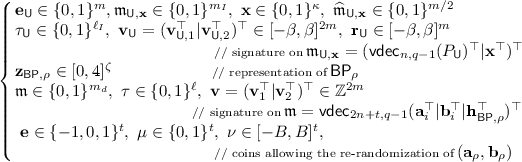
    satisfying the relations (modulo q)

    

    (11)

    and such that $\mathbf {z}_{\mathsf {BP},\rho } \in [0,4]^\zeta$ encodes $\mathsf {BP}_\rho$ such that $\mathsf {BP}_\rho (\mathbf {x})=1$. This is done by running the argument system described in Sect. 6.6.

  • 3. If the ZK argument of step 2 verifies, $\mathsf {DB}$ decrypts $(\mathbf {c}_0,\mathbf {c}_1) \in \mathbb {Z}_q^n \times \mathbb {Z}_q^t$ to obtain $M' = \lfloor (\mathbf {c}_1 - \mathbf {S}^\top \cdot \mathbf {c}_0) / ( q/2 ) \rceil \in \{0,1\}^t,$ which is returned to $\mathsf {U}$. Then, $\mathsf {DB}$ argues knowledge of $\mathbf {y}= \mathbf {c}_1 - \mathbf {S}^\top \cdot \mathbf {c}_0 - M' \cdot \lfloor q/2 \rfloor \in \mathbb {Z}^t$ of norm $\Vert \mathbf {y} \Vert _{\infty } \le q/5$ and small-norm $\mathbf {E}\in \mathbb {Z}^{m \times t}$, $\mathbf {S} \in \mathbb {Z}^{n \times t}$ satisfying (modulo q)

    $$\begin{aligned} \mathbf {P}= & {} \mathbf {F}^\top \cdot \mathbf {S} + \mathbf {E}, \qquad \mathbf {c}_0^\top \cdot \mathbf {S} + \mathbf {y}^\top = \mathbf {c}_1^\top - {M'}^\top \cdot \lfloor q/2 \rfloor . \end{aligned}$$

    To this end, $\mathsf {DB}$ uses the ZK argument system of Sect. 6.4.

  • 4. If the ZK argument produced by $\mathsf {DB}$ does not verify, $\mathsf {U}$ outputs $\perp$. Otherwise, $\mathsf {U}$ recalls the string $\mu \in \{0,1\}^t$ and outputs $M_{\rho _i}=M' \oplus \mu$.

Like our construction of Sect. 4, the above protocol requires the $\mathsf {DB}$ to repeat a ZK proof of communication complexity $\varOmega (N)$ with each user $\mathsf {U}$ during the initialization phase. By applying the Fiat-Shamir heuristic as shown in the full version of the paper, the cost of the initialization phase can be made independent of the number of users: the sender can publicize $\bigl ( PK_{\mathrm {DB}}, \{ER_i, \mathsf {BP}_i \}_{i=1}^N \bigr )$ along with a with a universally verifiable non-interactive proof of well-formedness.

The security of the above protocol against static corruptions is proved in the full version of the paper, under the $\mathsf {SIS}$ and $\mathsf {LWE}$ assumptions.

6 Our Zero-Knowledge Arguments of Knowledge

This section provides all the zero-knowledge arguments of knowledge (ZKAoK) used as building blocks in our two adaptive OT schemes. Our argument systems operate in the framework of Stern’s protocol [48], which was originally introduced in the context of code-based cryptography but has been developed [34,35,36, 38, 39].

In Sect. 6.1, we first recall Stern’s protocol in a generalized, abstract manner suggested in [34]. Then, using various transformations, we will demonstrate that all the required ZKAoKs can be obtained from this abstract protocol. Our basic strategy and techniques are summarized in Sect. 6.2, while the details of the protocols are given in the next subsections. In particular, our treatment of hidden branching programs in Sect. 6.6 is rather sophisticated as it requires to handle a number of secret objects nested together via branching programs, commitments, encryptions, signatures and Merkle trees. This protocol introduces new techniques and insights of which we provide the intuition hereafter.

6.1 Abstracting Stern’s Protocol

Let K, D, q be positive integers with $D \ge K$ and $q \ge 2$, and let $\mathsf {VALID}$ be a subset of $\mathbb {Z}^D$. Suppose that $\mathcal {S}$ is a finite set such that every $\phi \in \mathcal {S}$ can be associated with a permutation $\varGamma _\phi$ of D elements satisfying the following conditions:

$$\begin{aligned} {\left\{ \begin{array}{ll} \mathbf {w} \in \mathsf {VALID} \Longleftrightarrow \varGamma _\phi (\mathbf {w}) \in \mathsf {VALID}, \\ \text {If } \mathbf {w} \in \mathsf {VALID} \text { and } \phi \text { is uniform in } \mathcal {S}, \text { then } \varGamma _\phi (\mathbf {w}) \text { is uniform in } \mathsf {VALID}. \end{array}\right. } \end{aligned}$$

(12)

We aim to construct a statistical ZKAoK for the following abstract relation:

$$\begin{aligned} \mathrm {R_{abstract}} = \big \{ \big ((\mathbf {M}, \mathbf {v}), \mathbf {w} \big ) \in \mathbb {Z}_q^{K \times D} \times \mathbb {Z}_q^D \times \mathsf {VALID}: \mathbf {M}\cdot \mathbf {w} = \mathbf {v} \bmod q.\big \} \end{aligned}$$

Stern’s original protocol corresponds to the case $\mathsf {VALID} = \{ \mathbf {w} \in \{0,1\}^D: \mathsf {wt}(\mathbf {w}) = k\}$, where $\mathsf {wt}(\cdot )$ denotes the Hamming weight and $k < D$ is a given integer, $\mathcal {S} = \mathcal {S}_D$ is the set of all permutations of D elements and $\varGamma _{\phi }(\mathbf {w}) = \phi (\mathbf {w})$.

The conditions in (12) play a crucial role in proving in ZK that $\mathbf {w} \in \mathsf {VALID}$. To this end, the prover samples a random $\phi \hookleftarrow U(\mathcal {S})$ and lets the verifier check that $\varGamma _\phi (\mathbf {w}) \in \mathsf {VALID}$ without learning any additional information about $\mathbf {w}$ due to the randomness of $\phi$. Furthermore, to prove in a zero-knowledge manner that the linear equation is satisfied, the prover samples a masking vector $\mathbf {r}_w \hookleftarrow U(\mathbb {Z}_q^D)$, and convinces the verifier instead that $\mathbf {M}\cdot (\mathbf {w} + \mathbf {r}_w) = \mathbf {M}\cdot \mathbf {r}_w + \mathbf {v} \bmod q$.

The interaction between prover $\mathcal {P}$ and verifier $\mathcal {V}$ is described in Fig. 1. The protocol uses a statistically hiding and computationally binding string commitment scheme COM (e.g., the SIS-based scheme from [32]).

Fig. 1.

Stern-like ZKAoK for the relation $\mathrm {R_{abstract}}$.

Theorem 2

The protocol in Fig. 1 is a statistical ZKAoK with perfect completeness, soundness error 2 / 3, and communication cost $\mathcal {O}(D\log q)$. Namely:

• There exists a polynomial-time simulator that, on input $(\mathbf {M}, \mathbf {v})$, outputs an accepted transcript statistically close to that produced by the real prover.

• There exists a polynomial-time knowledge extractor that, on input a commitment $\mathrm {CMT}$ and 3 valid responses $(\mathrm {RSP}_1,\mathrm {RSP}_2,\mathrm {RSP}_3)$ to all 3 possible values of the challenge Ch, outputs $\mathbf {w}' \in \mathsf {VALID}$ such that $\mathbf {M}\cdot \mathbf {w}' = \mathbf {v} \bmod q.$

The proof of the theorem relies on standard simulation and extraction techniques for Stern-like protocols [32, 34, 38]. It is given in the full version of the paper.

6.2 Our Strategy and Basic Techniques, in a Nutshell

Before going into the details of our protocols, we first summarize our governing strategy and the techniques that will be used in the next subsections.

In each protocol, we prove knowledge of (possibly one-dimensional) integer vectors $\{\mathbf {w}_i\}_i$ that have various constraints (e.g., smallness, special arrangements of coordinates, or correlation with one another) and satisfy a system

(13)

where $\{\mathbf {M}_{i,j}\}_{i,j}$, $\{\mathbf {v}_j\}_{j}$ are public matrices (which are possibly zero or identity matrices) and vectors. Our strategy consists in transforming this entire system into one equivalent equation $\mathbf {M}\cdot \mathbf {w} = \mathbf {v}$, where matrix $\mathbf {M}$ and vector $\mathbf {v}$ are public, while the constraints of the secret vector $\mathbf {w}$ capture those of witnesses $\{\mathbf {w}_i\}_i$ and they are provable in zero-knowledge via random permutations. For this purpose, the Stern-like protocol from Sect. 6.1 comes in handy.

A typical transformation step is of the form $\mathbf {w}_i \rightarrow \bar{\mathbf {w}}_i$, where there exists public matrix $\mathbf {P}_{i,j}$ such that $\mathbf {P}_{i,j}\cdot \bar{\mathbf {w}}_i = \mathbf {w}_i$. This subsumes the decomposition and extension mechanisms which first appeared in [38].

• Decomposition: Used when $\mathbf {w}_i$ has infinity norm bound larger than 1 and we want to work more conveniently with $\bar{\mathbf {w}}_i$ whose norm bound is exactly 1. In this case, $\mathbf {P}_{i,j}$ is a decomposition matrix (see Sect. 2.5).

• Extension: Used when we insert “dummy” coordinates to $\mathbf {w}_i$ to obtain $\bar{\mathbf {w}}_i$ whose coordinates are somewhat balanced. In this case, $\mathbf {P}_{i,j}$ is a $\{0,1\}$-matrix with zero-columns corresponding to positions of insertions.

Such a step transforms the term $\mathbf {M}_{i,j}\cdot \mathbf {w}_i$ into $\overline{\mathbf {M}}_{i,j}\cdot \bar{\mathbf {w}}_i$, where $\overline{\mathbf {M}}_{i,j} = \mathbf {M}_{i,j}\cdot \mathbf {P}_{i,j}$ is a public matrix. Also, using the commutativity property of addition, we often group together secret vectors having the same constraints.

After a number of transformations, we will reach a system equivalent to (13):

$$\begin{aligned} {\left\{ \begin{array}{ll} \mathbf {M}'_{1,1}\cdot \mathbf {w}'_1 + \mathbf {M}'_{1,2}\cdot \mathbf {w}'_2 + \cdots + \mathbf {M}'_{1,k} \cdot \mathbf {w}'_{k} = \mathbf {v}_1, \\ \vdots \\ \mathbf {M}'_{t,1}\cdot \mathbf {w}'_1 + \mathbf {M}'_{t,2}\cdot \mathbf {w}'_2 + \cdots + \mathbf {M}'_{t,k} \cdot \mathbf {w}'_{k} = \mathbf {v}_t, \end{array}\right. } \end{aligned}$$

(14)

where integers t, k and matrices $\mathbf {M}'_{i,j}$ are public. Defining

we obtain the unified equation $\mathbf {M}\cdot \mathbf {w} = \mathbf {v} \bmod q$. At this stage, we will use a properly defined composition of random permutations to prove the constraints of $\mathbf {w}$. We remark that the crucial aspect of the above process is in fact the manipulation of witness vectors, while the transformations of public matrices/vectors just follow accordingly. To ease the presentation of the next subsections, we will thus only focus on the secret vectors.

In the process, we will employ various extending and permuting techniques which require introducing some notations. The most frequently used ones are given in Table 1. Some of these techniques appeared (in slightly different forms) in previous works [34,35,36, 38, 39]. The last three parts of the table summarizes newly-introduced techniques that will enable the treatment of secret-and-correlated objects involved in the evaluation of hidden branching programs.

In particular, the technique of the last row will be used for proving knowledge of an integer $z = x\cdot y$ for some $(x,y) \in [0,4] \times \{0,1\}$ satisfying other relations.

6.3 Protocol 1

Let $n, m, q, N, t, B_\chi$ be the parameters defined in Sect. 4. The protocol allows the prover to prove knowledge of LWE secrets and the well-formedness of ciphertexts. It is summarized as follows.

• Common input: $\mathbf {F} \in \mathbb {Z}_q^{n \times m}$, $\mathbf {P} \in \mathbb {Z}_q^{m \times t}$; $\{\mathbf {a}_i\in \mathbb {Z}_q^n, \mathbf {b}_i \in \mathbb {Z}_q^t\}_{i=1}^N$.

• Prover’s goal is to prove knowledge of $\mathbf {S} \in [-B_\chi ,B_\chi ]^{n \times t}$, $\mathbf {E} \in [-B_\chi ,B_\chi ]^{m \times t}$, $\{\mathbf {x}_i\in [-B_\chi ,B_\chi ]^t, M_i \in \{0,1\}^t\}_{i=1}^N$ such that the following equations hold:

(15)

For each $j \in [t]$, let $\mathbf {p}_j, \mathbf {s}_j, \mathbf {e}_j$ be the j-th column of matrices $\mathbf {P}, \mathbf {S}, \mathbf {E}$, respectively. For each $(i, j) \in [N]\times [t]$, let $\mathbf {b}_i[j], \mathbf {x}_i[j], M_i[j]$ denote the j-th coordinate of vectors $\mathbf {b}_i, \mathbf {x}_i, M_i$, respectively. Then, observe that (15) can be rewritten as:

(16)

Then, we form the following vectors:

$$\begin{aligned} \mathbf {w}_1= & {} \big ( \mathbf {s}_1^\top \mid \ldots \mid \mathbf {s}_t^\top \mid \mathbf {e}_1^\top \mid \ldots \mid \mathbf {e}_t^\top \mid ( \mathbf {x}_1[1], \ldots , \mathbf {x}_N[t]) \big )^\top \in [-B_\chi ,B_\chi ]^{(n+m+N)t}; \\ \mathbf {w}_2= & {} (M_1[1], \ldots , M_N[t])^\top \in \{0,1\}^{Nt}. \end{aligned}$$

Next, we run $\mathsf {vdec}'_{(n+m+N)t, B_\chi }$ to decompose $\mathbf {w}_1$ into $\bar{\mathbf {w}}_1$ and then extend $\bar{\mathbf {w}}_1$ to $\mathbf {w}_1^* \in \mathsf {B}_{(n+m+N)t\delta _{B_\chi }}^3$. We also extend $\mathbf {w}_2$ into $\mathbf {w}_2^* \in \mathsf {B}_{Nt}^2$ and we then form $\mathbf {w} = ((\mathbf {w}_1^*)^\top \mid (\mathbf {w}_2^*)^\top )^\top \in \{-1,0,1\}^D$, where $D = 3(n+m+N)t\delta _{B_\chi } + 2Nt$.

Observe that relations (16) can be transformed into one equivalent equation of the form $\mathbf {M}\cdot \mathbf {w} = \mathbf {v} \bmod q,$ where $\mathbf {M}$ and $\mathbf {v}$ are built from the common input.

Having performed the above unification, we now define $\mathsf {VALID}$ as the set of all vectors $\mathbf {t} = (\mathbf {t}_1^\top \mid \mathbf {t}_2^\top )^\top \in \{-1,0,1\}^D$, where $\mathbf {t}_1 \in \mathsf {B}_{(n+m+N)t\delta _{B_\chi }}^3$ and $\mathbf {t}_2 \in \mathsf {B}_{Nt}^2$. Clearly, our vector $\mathbf {w}$ belongs to the set $\mathsf {VALID}$.

Next, we specify the set $\mathcal {S}$ and permutations of D elements $\{\varGamma _\phi : \phi \in \mathcal {S}\}$, for which the conditions in (12) hold.

• $\mathcal {S}: = \mathcal {S}_{3(n+m+N)t\delta _{B_\chi }} \times \mathcal {S}_{2Nt}$.

• For $\phi = (\phi _1, \phi _2) \in \mathcal {S}$ and for $\mathbf {t} = (\mathbf {t}_1^\top \mid \mathbf {t}_2^\top )^\top \in \mathbb {Z}^D$, where $\mathbf {t}_1 \in \mathbb {Z}^{3(n+m+N)t\delta _{B_\chi }}$ and $\mathbf {t}_2 \in \mathbb {Z}^{2Nt}$, we define $\varGamma _\phi (\mathbf {t}) = (\phi _1(\mathbf {t}_1)^\top \mid \phi _2(\mathbf {t}_2)^\top )^\top$.

By inspection, it can be seen that the desired properties in (12) are satisfied. As a result, we can obtain the required ZKAoK by running the protocol from Sect. 6.1 with common input $(\mathbf {M}, \mathbf {v})$ and prover’s input $\mathbf {w}$. The protocol has communication cost $\mathcal {O}(D\log q)= \widetilde{\mathcal {O}}(\lambda )\cdot \mathcal {O}(Nt)$ bits.

Table 1. Basic notations and extending/permuting techniques used in our protocols.

While this protocol has linear complexity in N, it is only used in the initialization phase, where $\varOmega (N)$ bits inevitably have to be transmitted anyway.

6.4 Protocol 2

Let n, m, q, N, t, B be system parameters. The protocol allows the prover to prove knowledge of LWE secrets and the correctness of decryption.

• Common input: $\mathbf {F} \in \mathbb {Z}_q^{n \times m}$, $\mathbf {P} \in \mathbb {Z}_q^{m \times t}$; $\mathbf {c}_0 \in \mathbb {Z}_q^n, \mathbf {c}_1 \in \mathbb {Z}_q^t$, $M' \in \{0,1\}^t$.

• Prover’s goal is to prove knowledge of $\mathbf {S} \in [-B_\chi ,B_\chi ]^{n \times t}$, $\mathbf {E} \in [-B_\chi ,B_\chi ]^{m \times t}$ and $\mathbf {y} \in [-q/5, q/5]^{t}$ such that the following equations hold:

$$\begin{aligned} \mathbf {F}^\top \cdot \mathbf {S} + \mathbf {E} = \mathbf {P} \bmod q; \mathbf {c}_0^\top \cdot \mathbf {S} + \mathbf {y}^\top = \mathbf {c}_1^\top - M'^\top \cdot \lfloor q/2\rfloor \bmod q. \end{aligned}$$

(17)

For each $j \in [t]$, let $\mathbf {p}_j, \mathbf {s}_j, \mathbf {e}_j$ be the j-th column of matrices $\mathbf {P}, \mathbf {S}, \mathbf {E}$, respectively; and let $\mathbf {y}[j], \mathbf {c}_1[j], M'[j]$ be the j-th entry of vectors $\mathbf {y}, \mathbf {c}_1, M'$, respectively. Then, observe that (17) can be re-written as:

$$\begin{aligned} \forall j \in [t]: {\left\{ \begin{array}{ll} \mathbf {F}^\top \cdot \mathbf {s}_j + \mathbf {I}_m \cdot \mathbf {e}_j = \mathbf {p}_j \bmod q \\ \mathbf {c}_0^\top \cdot \mathbf {s}_j + 1\cdot \mathbf {y}[j] = \mathbf {c}_1[j]- M'[j]\cdot \lfloor q/2\rfloor \bmod q. \end{array}\right. } \end{aligned}$$

(18)

Next, we form vector $\mathbf {w}_1 = (\mathbf {s}_1^\top \mid \ldots \mid \mathbf {s}_t^\top \mid \mathbf {e}_1^\top \mid \ldots \mid \mathbf {e}_t^\top )^\top \in [-B_\chi ,B_\chi ]^{(n+m)t}$, then decompose it to $\bar{\mathbf {w}}_1 \in \{-1,0,1\}^{(n+m)t\delta _{B_\chi }}$, and extend $\bar{\mathbf {w}}_1$ to $\mathbf {w}_1^* \in \mathsf {B}_{(n+m)t\delta _{B_\chi }}^3$.

At the same time, we decompose vector $\mathbf {y} = (\mathbf {y}[1], \ldots , \mathbf {y}[t])^\top \in [-q/5, q/5]^{t}$ to $\bar{\mathbf {y}} \in \{-1,0,1\}^{t\delta _{q/5}}$, and then extend $\bar{\mathbf {y}}$ to $\mathbf {y}^* \in \mathsf {B}_{t\delta _{q/5}}^3$.

Defining the ternary vector $\mathbf {w} = ((\mathbf {w}^*_1)^\top \mid (\mathbf {y}^*)^\top )^\top \in \{-1,0,1\}^D$ of dimension $D = 3(n+m)t\delta _{B_\chi } + 3t\delta _{q/5}$, we finally obtain the equation $\mathbf {M}\cdot \mathbf {w} = \mathbf {v} \bmod q$, for public matrix $\mathbf {M}$ and public vector $\mathbf {v}$. Using similar arguments as in Sect. 6.3, we can obtain the desired zero-knowledge argument system. The protocol has communication cost $\mathcal {O}(D\log q)= \widetilde{\mathcal {O}}(\lambda )\cdot \mathcal {O}(t)$ bits.

6.5 Protocol 3

Let $n, m, m_d, q, t, \ell , B$ be the parameters defined in Sect. 4. The protocol allows the prover to argue that a given ciphertext is a correct randomization of some hidden ciphertext and that he knows a valid signature on that ciphertext. Let $\beta$ be the infinity norm bound of these valid signatures.

• Common input: It consists of matrices $\mathbf {F} \in \mathbb {Z}_q^{n \times m}$, $\mathbf {P} \in \mathbb {Z}_q^{m \times t}$, $\mathbf {A}, \mathbf {A}_0, \mathbf {A}_1,$ $\ldots , \mathbf {A}_\ell \in \mathbb {Z}_q^{n \times m}$, $\mathbf {D} \in \mathbb {Z}_q^{n \times m_d}$ and vectors $\mathbf {c}_0 \in \mathbb {Z}_q^n, \mathbf {c}_1 \in \mathbb {Z}_q^t, \mathbf {u} \in \mathbb {Z}_q^n$.

• Prover’s goal is to prove knowledge of $\mathfrak {m} \in \{0,1\}^{m_d}$, $\mu \in \{0,1\}^t$, $\mathbf {e} \in \{-1,0,1\}^t$, $\nu \in [-B,B]^t$, $\tau = (\tau [1], \ldots , \tau [\ell ])^\top \in \{0,1\}^\ell$, $\mathbf {v}_1, \mathbf {v}_2 \in [-\beta , \beta ]^m$ such that the following equations hold:

$$\begin{aligned} {\left\{ \begin{array}{ll} \mathbf {A}\cdot \mathbf {v}_1 + \mathbf {A}_0 \cdot \mathbf {v}_2 + \sum _{j=1}^\ell \mathbf {A}_j \cdot (\tau [j]\cdot \mathbf {v}_2) - \mathbf {D}\cdot \mathfrak {m} = \mathbf {u} \bmod q; \\ \mathbf {H}_{n+t, q-1}\cdot \mathfrak {m} + \left( \begin{array}{c} \mathbf {F} \\ \mathbf {P}^\top \\ \end{array} \right) \cdot \mathbf {e} + \left( \begin{array}{c} \mathbf {0}^{n \times t} \\ \lfloor \frac{q}{2}\rfloor \cdot \mathbf {I}_t\\ \end{array} \right) \cdot \mu + \left( \begin{array}{c} \mathbf {0}^{n \times t} \\ \mathbf {I}_t \\ \end{array} \right) \cdot \nu = \left( \begin{array}{c} \mathbf {c}_0 \\ \mathbf {c}_1 \\ \end{array} \right) \bmod q. \end{array}\right. } \end{aligned}$$

(19)

For this purpose, we perform the following transformations on the witnesses.

Decompositions. Decompose vectors $\mathbf {v}_1, \mathbf {v}_2, \nu$ to vectors $\bar{\mathbf {v}}_1 \in \{-1,0,1\}^{m\delta _\beta }$, $\bar{\mathbf {v}}_2 \in \{-1,0,1\}^{m\delta _\beta }$, $\bar{\nu } \in \{-1,0,1\}^{t\delta _B}$, respectively.

Extensions/Combinations.

• Let $\mathbf {w}_1 = (\mathfrak {m}^\top \mid \mu ^\top )^\top \in \{0,1\}^{m_d +t}$ and extend it into $\mathbf {w}_1^* \in \mathsf {B}_{m_d+t}^2$.

• Let $\mathbf {w}_2 = (\bar{\mathbf {v}}_1^\top \mid \bar{\nu }^\top \mid \mathbf {e}^\top )^\top \in \{-1,0,1\}^{m\delta _\beta + t\delta _B + t}$ and extend it into the vector $\mathbf {w}_2^* \in \mathsf {B}_{m\delta _\beta + t\delta _B + t}^3$.

• Extend $\bar{\mathbf {v}}_2$ into $\mathbf {s}_0 \in \mathsf {B}_{m\delta _\beta }^3$. Then, for each $j \in [\ell ]$, define ${\mathbf {s}}_j = \mathsf {expand}(\tau [j], \mathbf {s}_0)$. (We refer to Table 1 for details about $\mathsf {expand}(\cdot , \cdot )$.)

Now, we form vector $\mathbf {w} = \bigl ({\mathbf {w}_1^*}^\top \mid {\mathbf {w}_2^*}^\top \mid \mathbf {s}_0^\top \mid {\mathbf {s}}_1^\top \mid \ldots \mid {\mathbf {s}}_\ell ^\top \bigr )^\top \in \{-1,0,1\}^D$, where $D = (2\ell +2)3m\delta _\beta + 3t\delta _B + 3t + 2(m_d+t)$. At this point, we observe that the equations in (19) can be equivalently transformed into $\mathbf {M}\cdot \mathbf {w} = \mathbf {v} \bmod q$, where the matrix $\mathbf {M}$ and the vector $\mathbf {v}$ are built from the public input.

Having performed the above transformations, we now define $\mathsf {VALID}$ as the set of all vectors $\mathbf {t} = (\mathbf {t}_1^\top \mid \mathbf {t}_2^\top \mid \mathbf {t}_{3,0}^\top \mid \mathbf {t}_{3,1}^\top \mid \ldots \mid \mathbf {t}_{3,\ell }^\top )^\top \in \{-1,0,1\}^D$ for which there exists $\tau = (\tau [1], \ldots , \tau [\ell ])^\top \in \{0,1\}^\ell$ such that:

$$ \mathbf {t}_1 \in \mathsf {B}_{m_d+t}^2; \mathbf {t}_2 \in \mathsf {B}_{m\delta _\beta + t\delta _B + t}^3; \mathbf {t}_{3,0} \in \mathsf {B}_{m\delta _\beta }^3; \forall j\in [\ell ]: \mathbf {t}_{3,j} = \mathsf {expand}(\tau [j], \mathbf {t}_{3,0}). $$

It can be seen that $\mathbf {w}$ belongs to this tailored set. Now, let us specify the set $\mathcal {S}$ and permutations of D elements $\{\varGamma _\phi : \phi \in \mathcal {S}\}$ satisfying the conditions in (12).

• $\mathcal {S}: = \mathcal {S}_{2(m_d+t)} \times \mathcal {S}_{3(m\delta _\beta + t\delta _B + t)} \times \mathcal {S}_{3m\delta _\beta } \times \{0,1\}^\ell$.

• For $\phi = \big (\phi _1, \phi _2, \phi _{3}, (b[1], \ldots , b[\ell ])^\top \big ) \in \mathcal {S}$, we define the permutation $\varGamma _\phi$ that transforms vector $\mathbf {t} = (\mathbf {t}_1^\top \mid \mathbf {t}_2^\top \mid \mathbf {t}_{3,0}^\top \mid \mathbf {t}_{3,1}^T \mid \ldots \mid \mathbf {t}_{3,\ell }^\top )^\top \in \mathbb {Z}^D$ as follows:

  $$\begin{aligned} \varGamma _\phi (\mathbf {t}) = \big (\phi _1(\mathbf {t}_1)^\top \mid&\phi _2(\mathbf {t}_2)^\top \mid \phi _3(\mathbf {t}_{3,0})^\top \mid \\&T_{\mathsf {exp}}[b[1],\phi _3](\mathbf {t}_{3,1})^\top \mid \ldots \mid T_{\mathsf {exp}}[b[\ell ],\phi _3](\mathbf {t}_{3,\ell })^\top \big )^\top . \end{aligned}$$

By inspection, it can be seen that the properties in (12) are indeed satisfied. As a result, we can obtain the required argument of knowledge by running the protocol from Sect. 6.1 with common input $(\mathbf {M}, \mathbf {v})$ and prover’s input $\mathbf {w}$. The protocol has communication cost $\mathcal {O}(D\log q)= \widetilde{\mathcal {O}}(\lambda )\cdot \mathcal {O}(\log N + t)$ bits.

6.6 Protocol 4: A Treatment of Hidden Branching Programs

We now present the proof system run by the user in the OT-AC system of Sect. 5. It allows arguing knowledge of an input $\mathbf {x} = (x_0, \ldots , x_{\kappa -1})^\top \in \{0,1\}^\kappa$ satisfying a hidden branching program $\mathsf {BP}= \{(\mathrm {var}(\theta ),\pi _{\theta ,0},\pi _{\theta ,1})\}_{\theta =1}^L$ of length for $L \in \mathsf {poly}(\lambda )$. The prover should additionally demonstrate that: (i) He has a valid credential for $\mathbf {x}$; (ii) The hashed encoding of $\mathsf {BP}$ is associated with some hidden ciphertext of the database (and he knows a signature guaranteeing this link); (iii) A given ciphertext is a re-randomization of that hidden ciphertext.

Recall that, at each step $\theta \in [L]$ of the evaluation of $\mathsf {BP}(\mathbf {x})$, we have to look up the value $x_{\mathrm {var}(\theta )}$ in $\mathbf {x}=(x_0, \ldots , x_{\kappa -1})^\top$ to compute the $\theta$-th state $\eta _\theta$ as per

$$\begin{aligned} \eta _\theta = \pi _{\theta , x_{\mathrm {var}(\theta )}}(\eta _{\theta -1}) = \pi _{\theta , 0}(\eta _{\theta -1})\cdot \bar{x}_{\mathrm {var}(\theta )} + \pi _{\theta , 1}(\eta _{\theta -1})\cdot {x}_{\mathrm {var}(\theta )}. \end{aligned}$$

(20)

To prove that each step is done correctly, it is necessary to provide evidence that the corresponding search is honestly carried out without revealing ${x}_{\mathrm {var}(\theta )}$, ${\mathrm {var}(\theta )}$ nor $\{ \pi _{\theta ,b}\}_{b=0}^1$. To this end, a first idea is to perform a simple left-to-right search on $(x_0, \ldots , x_{\kappa -1})$: namely, (20) is expressed in terms of a matrix-vector relation where $\eta _\theta$ is encoded as a unit vector of dimension 5; $\{ \pi _{\theta ,b}\}_{b=0}^1$ are represented as permutation matrices; and $\mathbf {x}_{\mathrm {var}(\theta )} = \mathbf {M}_{\mathrm {var}(\theta )} \cdot \mathbf {x}$ is computed using a matrix $\mathbf {M}_{\mathrm {var}(\theta )} \in \{0,1\}^{\kappa \times \kappa }$ containing exactly one 1 per row. While this approach can be handled using proofs for matrix-vector relations using the techniques of [35], the expected complexity is $\mathcal {O}(\kappa )$ for each step, so that the total complexity becomes $\mathcal {O}(L \kappa )$. Fortunately, a better complexity can be achieved.

If we instead perform a dichotomic search on $\mathbf {x}=(x_0, \ldots , x_{\kappa -1})^\top$, we can reduce the complexity of each step to $\mathcal {O}(\log \kappa )$. To this end, we need to prove a statement “I performed a correct dichotomic search on my secret array $\mathbf {x}$”.

In order to solve this problem, we will employ two existing lattice-based tools:

• (i) A variant of the SIS-based computationally binding and statistically hiding commitment scheme from [32], which allows to commit to one-bit messages;

• (ii) The SIS-based Merkle hash tree proposed in [36].

Let $\bar{\mathbf {A}} \hookleftarrow U(\mathbb {Z}_q^{n \times m})$ and $\mathbf {a}_{\mathsf {com}} \hookleftarrow U(\mathbb {Z}_q^{n})$. For each $i \in [0,\kappa -1]$, we let the receiver commit to $x_i \in \{0,1\}$ as $\mathsf {com}_i = \mathbf {a}_{\mathsf {com}}\cdot x_i + \bar{\mathbf {A}}\cdot \mathbf {r}_{\mathsf {com},i}$, with $\mathbf {r}_{\mathsf {com},i} \hookleftarrow U(\{0,1\}^m)$, and reveal $\mathsf {com}_1,\ldots ,\mathsf {com}_{\kappa -1}$ to the sender. We build a Merkle tree of depth $\delta _\kappa = \lceil \log \kappa \rceil$ on top of the leaves $\mathsf {com}_0, \ldots , \mathsf {com}_{\kappa -1}$ using the $\mathsf {SIS}$-based hash function $h_{\bar{\mathbf {A}}}: \{0,1\}^{n\lceil \log q\rceil } \times \{0,1\}^{n\lceil \log q\rceil } \rightarrow \{0,1\}^{n\lceil \log q\rceil }$ of [36]. Our use of Merkle trees is reminiscent of [36] in that the content of the leaves is public. The Merkle tree will actually serve as a “bridge” ensuring that: (i) The same string $\mathbf {x}$ is used in all steps while enabling dichotomic searches; (ii) At each step, the prover indeed uses some coordinate of $\mathbf {x}$ (without revealing which one), the choice of which is dictated by a path in the tree determined by $\mathrm {var}(\theta )$.

Since $\{ \mathsf {com}_i \}_{i=0}^{\kappa -1}$ are public, both parties can deterministically compute the root $\mathbf {u}_{\mathsf {tree}}$ of the Merkle tree. For each $\theta \in [L]$, we consider the binary representation $d_{\theta , 1}, \ldots , d_{\theta , \delta _\kappa }$ of $\mathrm {var}(\theta )$, which is part of the encoding of $\mathsf {BP}$ defined in (7). We then prove knowledge of a bit $y_\theta$ satisfying the statement “From the root $\mathbf {u}_{\mathsf {tree}} \in \{0,1\}^{n\lceil \log q\rceil }$ of the tree, the path determined by the bits $d_{\theta , 1}, \ldots , d_{\theta , \delta _\kappa }$ leads to the leaf associated with the commitment opened to $y_\theta$.” If the Merkle tree and the commitment scheme are both secure, it should hold that $y_\theta = x_{\mathrm {var}(\theta )}$. Said otherwise, we can provably perform a “dichotomic search” for $x_{\mathrm {var}(\theta )} = y_\theta$. Moreover, the techniques from [36] can be adapted to do this in zero-knowledge manner, i.e., without revealing the path nor the reached leaf.

Now, our task can be divided into 3 steps: (i) Proving that the searches on Merkle tree yield $y_{1}, \ldots , y_L$; (ii) Proving that the branching program evaluates to $\mathsf {BP}(\mathbf {x})=1$ if $y_{1}, \ldots , y_L$ are used in the evaluation; (iii) Proving all the other relations mentioned above, as well as the consistency of $\{ \mathsf {com}_i \}_{i=0}^{\kappa -1}$ and the fact that they open to a certified $\mathbf {x} \in \{0,1\}^\kappa$.

Thanks to dichotomic searches, the communication cost drops to $\mathcal {O}(L \delta _\kappa + \kappa )$. These steps can be treated as explained below.

The Merkle Tree Step. At each step $\theta \in [L]$, the prover proves knowledge of a path made of $\delta _\kappa$ nodes $\mathbf {g}_{\theta ,1}, \ldots , \mathbf {g}_{\theta , \delta _\kappa } \in \{0,1\}^{n\lceil \log q\rceil }$ determined by $d_{\theta , 1}, \ldots , d_{\theta , \delta _\kappa }$, as well as their siblings $\mathbf {t}_{\theta , 1}, \ldots , \mathbf {t}_{\theta , \delta _\kappa } \in \{0,1\}^{n\lceil \log q\rceil }$. Also, the prover argues knowledge of an opening $(y_\theta , \mathbf {r}_\theta ) \in \{0,1\} \times \{0,1\}^m$ for the commitment of which $\mathbf {g}_{\theta , \delta _\kappa }$ is a binary decomposition. As shown in [36] (and recalled in the full paper), it suffices to prove the following relations (mod q):

(21)

where $\mathsf {expand}(\cdot , \cdot )$ is defined in Table 1.

Extending.

• For each $(\theta , i) \in [L] \times [\delta _\kappa ]$: Extend $\mathbf {g}_{\theta ,i}, \mathbf {t}_{\theta ,i} \in \{0,1\}^{m/2}$ to $\widetilde{\mathbf {g}}_{\theta ,i}, \widetilde{\mathbf {t}}_{\theta ,i} \in \mathsf {B}_{m/2}^2$, respectively. Then, let $\widehat{\mathbf {g}}_{\theta ,i} = \mathsf {expand}(d_{\theta ,i}, \widetilde{\mathbf {g}}_{\theta ,i})$ and $\widehat{\mathbf {t}}_{\theta ,i} = \mathsf {expand}(\bar{d}_{\theta ,i}, \widetilde{\mathbf {t}}_{\theta ,i})$.

• For each $\theta \in [L]$, extend the bit $y_\theta$ into the vector $\mathbf {y}_\theta = \mathsf {ext}_2(y_\theta ) \in \{0,1\}^2$.

• Let $\widetilde{\mathbf {r}} = (\mathbf {r}_1^\top \mid \ldots \mid \mathbf {r}_L^\top )^\top \in \{0,1\}^{mL}$, then extend it into the vector $\widehat{\mathbf {r}} \in \mathsf {B}_{mL}^2$.

Combining. Next, we let $D_{\mathsf {tree}} = 5mL\delta _\kappa + 2L + 2mL$ and define

$$\begin{aligned} \mathbf {w}_{\mathsf {tree}} = \bigl ( \widetilde{\mathbf {g}}_{1,1}^\top \mid \widehat{\mathbf {g}}_{1,1}^\top \mid \widehat{\mathbf {t}}_{1,1}^\top \mid \ldots \mid \widetilde{\mathbf {g}}_{1,\delta _\kappa }^\top \mid \widehat{\mathbf {g}}_{1,\delta _\kappa }^\top \mid \widehat{\mathbf {t}}_{1,\delta _\kappa }^\top \mid \ldots \mid \widetilde{\mathbf {g}}_{L,1}^\top \mid \widehat{\mathbf {g}}_{L,1}^\top \mid \widehat{\mathbf {t}}_{L,1}^\top \nonumber \\ \mid \ldots \mid \widetilde{\mathbf {g}}_{L,\delta _\kappa }^\top \mid \widehat{\mathbf {g}}_{L,\delta _\kappa }^\top \mid \widehat{\mathbf {t}}_{L,\delta _\kappa }^\top \mid \mathbf {y}_1^\top \mid \ldots \mid \mathbf {y}_L^\top \mid \widehat{\mathbf {r}}^\top \bigr )^\top \in \{0,1\}^{D_{\mathsf {tree}}}. \qquad \end{aligned}$$

(22)

Then, observe that, the above $L(\delta _\kappa +1)$ equations can be combined into one:

$$\begin{aligned} \mathbf {M}_{\mathsf {tree}}\cdot \mathbf {w}_{\mathsf {tree}} = \mathbf {v}_{\mathsf {tree}} \bmod q, \end{aligned}$$

(23)

where matrix $\mathbf {M}_{\mathsf {tree}}$ and vector $\mathbf {v}_{\mathsf {tree}}$ are built from the public input.

The Branching Program Step. The last three parts of Table 1 describe the vector transformations that will be used to handle the secret vectors appearing in the evaluation of $\mathsf {BP}$. The following equations emulate the evaluation process. In particular, for each $\theta \in [2,L]$, we introduce an extra vector $\mathbf {e}_\theta = (c_{\theta ,0}, \ldots , c_{\theta ,4}) \in \{0,1\}^5$ to enable the extraction of the values $\pi _{\theta , 0}(\eta _{\theta -1})$, and $\pi _{\theta ,1}(\eta _{\theta -1})$.

(24)

Extending.

• For each $\theta \in [L-1]$, extend $\eta _\theta \in [0, 4]$ to 5-dimensional vector $\mathbf {s}_\theta = \mathsf {ext}_5(\eta _\theta )$.

• For each $(\theta , j) \in [2, L] \times \{0,1\}$, extend $f_{\theta , j} \in [0, 4]$ to $\mathbf {f}_{\theta , j} = \mathsf {ext}_5(f_{\theta , j})$.

• For each $(\theta , i) \in [2,L] \times [0, 4]$, extend $c_{\theta , i} \in \{0,1\}$ to $\mathbf {c}_{\theta ,i} = \mathsf {ext}_2(c_{\theta , i})$.

• Extend the products $\pi _{1,0}(0)\cdot \bar{y}_1$ and $\pi _{1,1}(0)\cdot y_1$ into 10-dimensional vectors $\mathbf {h}_{1,0}= \mathsf {ext}_{5 \times 2}(\pi _{1,0}(0), \bar{y}_1)$ and $\mathbf {h}_{1,1} = \mathsf {ext}_{5 \times 2}(\pi _{1,1}(0), y_1)$, respectively.

• For each $\theta \in [2, L]$, extend the products $f_{\theta , 0}\cdot \bar{y}_\theta$ and $f_{\theta , 1}\cdot {y}_\theta$ into 10-dimensional vectors $\mathbf {h}_{\theta ,0}= \mathsf {ext}_{5 \times 2}(f_{\theta , 0}, \bar{y}_\theta )$ and $\mathbf {h}_{\theta ,1} = \mathsf {ext}_{5 \times 2}(f_{\theta , 1}, y_\theta )$.

• For $(\theta , i) \in [2,L] \times [0, 4]$, extend the products $\pi _{\theta , 0}(i)\cdot c_{\theta , i}$ and $\pi _{\theta , 1}(i)\cdot c_{\theta , i}$ into $\mathbf {z}_{\theta , 0, i} = \mathsf {ext}_{5 \times 2}(\pi _{\theta , 0}(i), c_{\theta , i})$ and $\mathbf {z}_{\theta , 1, i} = \mathsf {ext}_{5 \times 2}(\pi _{\theta , 1}(i), c_{\theta , i})$, respectively.

Combining. Let $D_{\mathsf {BP}}= 150L - 130$, and form $\mathbf {w}_{\mathsf {BP}} \in [0, 4]^{D_{\mathsf {BP}}}$ of the form:

$$\begin{aligned} \big ( \mathbf {s}_1^\top \mid \ldots \mid &\mathbf {s}_{L-1}^\top \mid \mathbf {e}_2^\top \mid \ldots \mid \mathbf {e}_L^\top \mid \mathbf {c}_{2,0}^\top \mid \ldots \mid \mathbf {c}_{L,4}^\top \mid \mathbf {z}_{2,0,0}^\top \mid \ldots \mid \mathbf {z}_{L,1,4}^\top \mid \nonumber \\&\mathbf {f}_{2,0}^\top \mid \ldots \mid \mathbf {f}_{L,1}^\top \mid \mathbf {h}_{1,0}^\top \mid \mathbf {h}_{1,1}^\top \mid \mathbf {h}_{2,0}^\top \mid \mathbf {h}_{2,1}^\top \mid \ldots \mid \mathbf {h}_{L,0}^\top \mid \mathbf {h}_{L,1}^\top \big )^\top . \qquad ~ \end{aligned}$$

(25)

Then, observe that the vector $\mathbf {w}_{\mathsf {BP}}$ of (25) satisfies one equation of the form:

$$\begin{aligned} \mathbf {M}_{\mathsf {BP}}\cdot \mathbf {w}_{\mathsf {BP}} = \mathbf {v}_{\mathsf {BP}}, \end{aligned}$$

(26)

where matrix $\mathbf {M}_{\mathsf {BP}}$ and vector $\mathbf {v}_{\mathsf {BP}}$ are obtained from the common input. Note that we work with integers in [0, 4], which are much smaller than q. As a result,

$$\begin{aligned} \mathbf {M}_{\mathsf {BP}}\cdot \mathbf {w}_{\mathsf {BP}} = \mathbf {v}_{\mathsf {BP}} \bmod q. \end{aligned}$$

(27)

Conversely, if we can prove that (27) holds for a well-formed vector $\mathbf {w}_{\mathsf {BP}}$, then that vector should also satisfy (26).

The Third Step. In the third layer, we have to prove knowledge of:

$$\begin{aligned} {\left\{ \begin{array}{ll} d_{1,1}, \ldots , d_{L, \delta _\kappa } \in \{0,1\}, \pi _{1,0}(0), \ldots , \pi _{L,1}(4) \in [0, 4],\mathfrak {m} \in \{0,1\}^{m_d}, \\ \mathbf {x} = (x_0, \ldots , x_{\kappa -1})^\top \in \{0,1\}^\kappa , \mathfrak {m}_{\mathsf {U}, \mathbf {x}} \in \{0,1\}^{\frac{m}{2} + \kappa }, \widehat{\mathfrak {m}}_{\mathsf {U}, \mathbf {x}} \in \{0,1\}^{\frac{m}{2}}, \\ \mathbf {e}_{\mathsf {U}} \in \{0,1\}^m, \mathbf {r}_{\mathsf {com},0}, \ldots , \mathbf {r}_{\mathsf {com},\kappa -1} \in \{0,1\}^m, \mu \in \{0,1\}^t, \tau \in \{0,1\}^\ell , \\ [2.6pt] \tau _{\mathsf {U}} \in \{0,1\}^{\ell _I}, \mathbf {v}_1, \mathbf {v}_2, \mathbf {v}_{\mathsf {U},1}, \mathbf {v}_{\mathsf {U},2}, \mathbf {r}_{\mathsf {U}} \in [-\beta ,\beta ]^m, \mathbf {e} \in \{-1,0,1\}^t, \nu \in [-B,B]^t, \end{array}\right. } \end{aligned}$$

(28)

which satisfy the equations of (11) for $\mathbf {z}_{\mathsf {BP}, \rho } = (d_{1,1}, \ldots , d_{L, \delta _\kappa }, \pi _{1,0}(0), \ldots , \pi _{L,1}(4))^\top$ and, $\forall i \in [0,\kappa -1]$, the bit $x_i$ is committed in $\mathsf {com}_i$ with randomness $\mathbf {r}_{\mathsf {com},i}$:

$$ \left[ \begin{array}{ccc} \mathbf {a}_{\mathsf {com}} &{} &{} \\ &{} \ddots &{} \\ &{} &{} \mathbf {a}_{\mathsf {com}} \\ \end{array} \right] \cdot \mathbf {x} + \left[ \begin{array}{ccc} \bar{\mathbf {A}} &{} &{} \\ &{} \ddots &{} \\ &{} &{} \bar{\mathbf {A}} \\ \end{array} \right] \cdot \left( \begin{array}{c} \mathbf {r}_{\mathsf {com},0} \\ \vdots \\ \mathbf {r}_{\mathsf {com},\kappa -1} \\ \end{array} \right) = \left( \begin{array}{c} \mathsf {com}_0 \\ \vdots \\ \mathsf {com}_{\kappa -1} \\ \end{array} \right) \bmod q. $$

Decomposing. We use $\mathsf {vdec}'_{m, \beta }(\cdot )$ to decompose $\mathbf {v}_1, \mathbf {v}_2, \mathbf {v}_{\mathsf {U},1}, \mathbf {v}_{\mathsf {U},2}, \mathbf {r}_{\mathsf {U}} \in [-\beta , \beta ]^m$ into $\bar{\mathbf {v}}_1, \bar{\mathbf {v}}_2, \bar{\mathbf {v}}_{\mathsf {U},1}, \bar{\mathbf {v}}_{\mathsf {U},2}, \bar{\mathbf {r}}_{\mathsf {U}} \in \{-1,0,1\}^{m\delta _\beta }$, respectively. Similarly, we decompose vector $\nu \in [-B,B]^t$ into vector $\bar{\nu } = \mathsf {vdec}'_{t,B}(\nu ) \in \{-1,0,1\}^{t\delta _B}$.

Extending and Combining. Next, we perform the following steps:

• For each $(\theta , i) \in [L] \times [\delta _\kappa ]$, extend $d_{\theta , i}$ to $\mathbf {d}_{\theta ,i} = \mathsf {ext}_2(d_{\theta ,i})$.

• For each $(\theta , j,i) \in [L] \times \{0,1\} \times [0, 4]$, extend $\pi _{\theta , j}(i)$ to $\varPi _{\theta , j,i} = \mathsf {ext}_5(\pi _{\theta , j}(i))$.

• Let $\overline{\mathbf {w}}_{3,1} = \big (\mathbf {x}^\top | \mathbf {r}_{\mathsf {com},0}^\top | \ldots | \mathbf {r}_{\mathsf {com},\kappa -1}^\top | \mathfrak {m}_{\mathsf {U}, \mathbf {x}}^\top | \widehat{\mathfrak {m}}_{\mathsf {U}, \mathbf {x}}^\top | \mathfrak {m}^\top \mid \mathbf {e}_{\mathsf {U}}^\top | \mu ^\top \big )^\top \in \{0,1\}^{D_{3,1}}$, where $D_{3,1} = \kappa (m +2) + 2m + m_d + t$. Then extend $\overline{\mathbf {w}}_{3,1}$ to ${\mathbf {w}}_{3,1} \in \mathsf {B}_{D_{3,1}}^2$.

• Define the vector $\overline{\mathbf {w}}_{3,2} = (\bar{\mathbf {v}}_1^\top | \bar{\mathbf {v}}_{\mathsf {U},1}^\top | \bar{\mathbf {r}}_{\mathsf {U}}^\top | \bar{\nu }^\top | \mathbf {e}^\top )^\top \in \{-1,0,1\}^{D_{3,2}}$ of dimension $D_{3,2} = 3m\delta _\beta + t(\delta _B+1)$ and extend it into ${\mathbf {w}}_{3,2} \in \mathsf {B}_{D_{3,2}}^3$.

• Extend $\bar{\mathbf {v}}_2$ to $\mathbf {s}_0 \in \mathsf {B}_{m\delta _\beta }^3$. Then for $j \in [\ell ]$, form vector $\mathsf {s}_j = \mathsf {expand}\big (\tau [j], \mathbf {s}_0\big )$.

• Extend $\bar{\mathbf {v}}_{\mathsf {U},2}$ to $\mathbf {s}_{\mathsf {U},0} \in \mathsf {B}_{m\delta _\beta }^3$. Then for $j \in [\ell _I]$, form $\mathsf {s}_{\mathsf {U},j} = \mathsf {expand}\big (\tau _{\mathsf {U}}[j], \mathbf {s}_{\mathsf {U},0}\big )$.

Given the above transformations, let $D_3 = 2L(\delta _\kappa +25) + 2D_{3,1} + 3D_{3,2} + 3m\delta _\beta (2\ell +1) + 3m\delta _\beta (2\ell _I+1)$ and construct vector $\mathbf {w}_3 \in [-1,4]^{D_3}$ of the form:

$$\begin{aligned} \big ( \mathbf {d}_{1,1}^\top \mid \ldots \mid \mathbf {d}_{L, \delta _\kappa }^\top&\mid \varPi _{1,0,0}^\top \mid \ldots \mid \varPi _{L,1,4}^\top \mid \mathbf {w}_{3,1}^\top \mid \mathbf {w}_{3,2}^\top \mid \nonumber \\&\mathbf {s}_0^\top \mid \mathbf {s}_1^\top \mid \ldots \mid \mathbf {s}_\ell ^\top \mid \mathbf {s}_{\mathsf {U},0}^\top \mid \mathbf {s}_{\mathsf {U},1}^\top \mid \ldots \mid \mathbf {s}_{\mathsf {U},\ell _I}^\top \mid \big )^\top . \qquad \end{aligned}$$

(29)

Observe that the given five equations can be combined into one of the form:

$$\begin{aligned} \mathbf {M}_3 \cdot \mathbf {w}_3 = \mathbf {v}_3 \bmod q, \end{aligned}$$

(30)

where matrix $\mathbf {M}_3$ and vector $\mathbf {v}_3$ can be built from the public input.

Putting Pieces Altogether. At the final stage of the process, we connect the three aforementioned steps. Indeed, all the equations involved in our process are captured by (23), (27), and (30) - which in turn can be combined into:

$$\begin{aligned} \mathbf {M}\cdot \mathbf {w} = \mathbf {v} \bmod q, \end{aligned}$$

(31)

where $\mathbf {w} = (\mathbf {w}_{\mathsf {tree}}^\top \mid \mathbf {w}_{\mathsf {BP}}^\top \mid \mathbf {w}_3^\top )^\top \in [-1,4]^D$, for

$$D = D_{\mathsf {tree}} + D_{\mathsf {BP}} + D_3 = \widetilde{\mathcal {O}}(\lambda )\cdot (L\cdot \log \kappa + \kappa ) + \widetilde{\mathcal {O}}(\lambda )\cdot (\log N + \lambda ) + \widetilde{\mathcal {O}}(1)\cdot t.$$

The components of $\mathbf {w}$ all have constraints listed in Table 1. By construction, these blocks either belong to the special sets $\mathsf {B}_{\mathfrak {m}}^2$, $\mathsf {B}_{\mathfrak {m}}^3$ or they have the special forms $\mathsf {expand}(\cdot , \cdot )$, $\mathsf {ext}_2(\cdot )$, $\mathsf {ext}_5(\cdot )$, $\mathsf {ext}_{5\times 2}(\cdot , \cdot )$, which are invariant under the permutations defined in Table 1. As a result, we can specify suitable sets $\mathsf {VALID}$, $\mathcal {S}$ and permutations of D elements $\{\varGamma _\phi : \phi \in \mathcal {S}\}$, for which the conditions of (12) are satisfied. The description of $\mathsf {VALID}$, $\mathcal {S}$ and $\varGamma _{\phi }$ is detailed in the full paper.

Our desired argument system then works as follows. At the beginning of the interaction, the prover computes commitments $\mathsf {com}_0, \ldots , \mathsf {com}_{\kappa -1} \in \mathbb {Z}_q^n$ and send them once to the verifier. Both parties construct matrix $\mathbf {M}$ and vector $\mathbf {v}$ based on the public input as well as $\mathsf {com}_0, \ldots , \mathsf {com}_{\kappa -1}$, while the prover prepares vector $\mathbf {w}$, as described. Finally, they run the protocol of Sect. 6.1, which has communication cost $\mathcal {O}(D \log q)= \mathcal {O}(L\cdot \log \kappa + \kappa )$.

References

Abe, M., Camenisch, J., Dubovitskaya, M., Nishimaki, R.: Universally composable adaptive oblivious transfer (with access control) from standard assumptions. In: ACM Workshop on Digital Identity Management (2013)
Agrawal, S., Boneh, D., Boyen, X.: Efficient lattice (H)IBE in the standard model. In: Gilbert, H. (ed.) EUROCRYPT 2010. LNCS, vol. 6110, pp. 553–572. Springer, Heidelberg (2010). https://doi.org/10.1007/978-3-642-13190-5_28
Aiello, B., Ishai, Y., Reingold, O.: Priced oblivious transfer: how to sell digital goods. In: Pfitzmann, B. (ed.) EUROCRYPT 2001. LNCS, vol. 2045, pp. 119–135. Springer, Heidelberg (2001). https://doi.org/10.1007/3-540-44987-6_8
Alwen, J., Peikert, C.: Generating shorter bases for hard random lattices. In: STACS 2009 (2009)
Asharov, G., Jain, A., López-Alt, A., Tromer, E., Vaikuntanathan, V., Wichs, D.: Multiparty computation with low communication, computation and interaction via threshold FHE. In: Pointcheval, D., Johansson, T. (eds.) EUROCRYPT 2012. LNCS, vol. 7237, pp. 483–501. Springer, Heidelberg (2012). https://doi.org/10.1007/978-3-642-29011-4_29
Barrington, D.: Bounded-width polynomial-size branching programs recognize exactly those languages in NC1. In: STOC 1986 (1986)
Böhl, F., Hofheinz, D., Jager, T., Koch, J., Striecks, C.: Confined guessing: new signatures from standard assumptions. J. Cryptol. 28(1), 176–208 (2015)
Boneh, D., Boyen, X.: Efficient selective-ID secure identity-based encryption without random Oracles. In: Cachin, C., Camenisch, J.L. (eds.) EUROCRYPT 2004. LNCS, vol. 3027, pp. 223–238. Springer, Heidelberg (2004). https://doi.org/10.1007/978-3-540-24676-3_14
Brakerski, Z., Langlois, A., Peikert, C., Regev, O., Stehlé, D.: On the classical hardness of learning with errors. In: STOC (2013)
Camenisch, J., Dubovitskaya, M., Enderlein, R.R., Neven, G.: Oblivious transfer with hidden access control from attribute-based encryption. In: Visconti, I., Prisco, R. (eds.) SCN 2012. LNCS, vol. 7485, pp. 559–579. Springer, Heidelberg (2012). https://doi.org/10.1007/978-3-642-32928-9_31
Camenisch, J., Dubovitskaya, M., Neven, G.: Oblivious transfer with access control. In: ACM-CCS 2009 (2009)
Camenisch, J., Dubovitskaya, M., Neven, G., Zaverucha, G.M.: Oblivious transfer with hidden access control policies. In: Catalano, D., Fazio, N., Gennaro, R., Nicolosi, A. (eds.) PKC 2011. LNCS, vol. 6571, pp. 192–209. Springer, Heidelberg (2011). https://doi.org/10.1007/978-3-642-19379-8_12
Camenisch, J., Neven, G., Shelat, A.: Simulatable adaptive oblivious transfer. In: Naor, M. (ed.) EUROCRYPT 2007. LNCS, vol. 4515, pp. 573–590. Springer, Heidelberg (2007). https://doi.org/10.1007/978-3-540-72540-4_33
Canetti, R.: Universally composable security: a new paradigm for cryptographic protocols. In: FOCS 2001 (2001)
Cash, D., Hofheinz, D., Kiltz, E., Peikert, C.: Bonsai trees, or how to delegate a lattice basis. In: Gilbert, H. (ed.) EUROCRYPT 2010. LNCS, vol. 6110, pp. 523–552. Springer, Heidelberg (2010). https://doi.org/10.1007/978-3-642-13190-5_27
Chor, B., Goldreich, O., Kushilevitz, E., Sudan, M.: Private information retrieval. In: FOCS 1995 (1995)
Coull, S., Green, M., Hohenberger, S.: Controlling access to an oblivious database using stateful anonymous credentials. In: Jarecki, S., Tsudik, G. (eds.) PKC 2009. LNCS, vol. 5443, pp. 501–520. Springer, Heidelberg (2009). https://doi.org/10.1007/978-3-642-00468-1_28
Crescenzo, G., Ostrovsky, R., Rajagopalan, S.: Conditional oblivious transfer and timed-release encryption. In: Stern, J. (ed.) EUROCRYPT 1999. LNCS, vol. 1592, pp. 74–89. Springer, Heidelberg (1999). https://doi.org/10.1007/3-540-48910-X_6
Ducas, L., Stehlé, D.: Sanitization of FHE ciphertexts. In: Fischlin, M., Coron, J.-S. (eds.) EUROCRYPT 2016. LNCS, vol. 9665, pp. 294–310. Springer, Heidelberg (2016). https://doi.org/10.1007/978-3-662-49890-3_12
Even, S., Goldreich, O., Lempel, A.: A randomized protocol for signing contracts. Commun. ACM 28(6), 637–647 (1985)
Fiat, A., Shamir, A.: How to prove yourself: practical solutions to identification and signature problems. In: Odlyzko, A.M. (ed.) CRYPTO 1986. LNCS, vol. 263, pp. 186–194. Springer, Heidelberg (1987). https://doi.org/10.1007/3-540-47721-7_12
Gentry, C., Peikert, C., Vaikuntanathan, V.: Trapdoors for hard lattices and new cryptographic constructions. In: STOC (2008)
Gentry, C., Sahai, A., Waters, B.: Homomorphic encryption from learning with errors: conceptually-simpler, asymptotically-faster, attribute-based. In: Canetti, R., Garay, J.A. (eds.) CRYPTO 2013. LNCS, vol. 8042, pp. 75–92. Springer, Heidelberg (2013). https://doi.org/10.1007/978-3-642-40041-4_5
Goldreich, O., Micali, S., Wigderson, A.: How to play any mental game or a completeness theorem for protocols with honest majority. In: STOC (1987)
Gorbunov, S., Vinayagamurthy, D.: Riding on asymmetry: efficient ABE for branching programs. In: Iwata, T., Cheon, J.H. (eds.) ASIACRYPT 2015. LNCS, vol. 9452, pp. 550–574. Springer, Heidelberg (2015). https://doi.org/10.1007/978-3-662-48797-6_23
Green, M., Hohenberger, S.: Blind identity-based encryption and simulatable oblivious transfer. In: Kurosawa, K. (ed.) ASIACRYPT 2007. LNCS, vol. 4833, pp. 265–282. Springer, Heidelberg (2007). https://doi.org/10.1007/978-3-540-76900-2_16
Green, M., Hohenberger, S.: Universally composable adaptive oblivious transfer. In: Pieprzyk, J. (ed.) ASIACRYPT 2008. LNCS, vol. 5350, pp. 179–197. Springer, Heidelberg (2008). https://doi.org/10.1007/978-3-540-89255-7_12
Green, M., Hohenberger, S.: Practical adaptive oblivious transfer from simple assumptions. In: Ishai, Y. (ed.) TCC 2011. LNCS, vol. 6597, pp. 347–363. Springer, Heidelberg (2011). https://doi.org/10.1007/978-3-642-19571-6_21
Herranz, J.: Restricted adaptive oblivious transfer. Theoret. Comput. Sci. 412(46), 6498–6506 (2011)
Hiromasa, R., Abe, M., Okamoto, T.: Packing messages and optimizing bootstrapping in GSW-FHE. In: Katz, J. (ed.) PKC 2015. LNCS, vol. 9020, pp. 699–715. Springer, Heidelberg (2015). https://doi.org/10.1007/978-3-662-46447-2_31
Jarecki, S., Liu, X.: Efficient oblivious pseudorandom function with applications to adaptive OT and secure computation of set intersection. In: Reingold, O. (ed.) TCC 2009. LNCS, vol. 5444, pp. 577–594. Springer, Heidelberg (2009). https://doi.org/10.1007/978-3-642-00457-5_34
Kawachi, A., Tanaka, K., Xagawa, K.: Concurrently secure identification schemes based on the worst-case hardness of lattice problems. In: Pieprzyk, J. (ed.) ASIACRYPT 2008. LNCS, vol. 5350, pp. 372–389. Springer, Heidelberg (2008). https://doi.org/10.1007/978-3-540-89255-7_23
Kurosawa, K., Nojima, R., Phong, L.T.: Generic fully simulatable adaptive oblivious transfer. In: Lopez, J., Tsudik, G. (eds.) ACNS 2011. LNCS, vol. 6715, pp. 274–291. Springer, Heidelberg (2011). https://doi.org/10.1007/978-3-642-21554-4_16
Libert, B., Ling, S., Mouhartem, F., Nguyen, K., Wang, H.: Signature schemes with efficient protocols and dynamic group signatures from lattice assumptions. In: Cheon, J.H., Takagi, T. (eds.) ASIACRYPT 2016. LNCS, vol. 10032, pp. 373–403. Springer, Heidelberg (2016). https://doi.org/10.1007/978-3-662-53890-6_13
Libert, B., Ling, S., Mouhartem, F., Nguyen, K., Wang, H.: Zero-knowledge arguments for matrix-vector relations and lattice-based group encryption. In: Cheon, J.H., Takagi, T. (eds.) ASIACRYPT 2016. LNCS, vol. 10032, pp. 101–131. Springer, Heidelberg (2016). https://doi.org/10.1007/978-3-662-53890-6_4
Libert, B., Ling, S., Nguyen, K., Wang, H.: Zero-knowledge arguments for lattice-based accumulators: logarithmic-size ring signatures and group signatures without trapdoors. In: Fischlin, M., Coron, J.-S. (eds.) EUROCRYPT 2016. LNCS, vol. 9666, pp. 1–31. Springer, Heidelberg (2016). https://doi.org/10.1007/978-3-662-49896-5_1
Lindell, A.Y.: Efficient fully-simulatable oblivious transfer. In: Malkin, T. (ed.) CT-RSA 2008. LNCS, vol. 4964, pp. 52–70. Springer, Heidelberg (2008). https://doi.org/10.1007/978-3-540-79263-5_4
Ling, S., Nguyen, K., Stehlé, D., Wang, H.: Improved zero-knowledge proofs of knowledge for the ISIS problem, and applications. In: Kurosawa, K., Hanaoka, G. (eds.) PKC 2013. LNCS, vol. 7778, pp. 107–124. Springer, Heidelberg (2013). https://doi.org/10.1007/978-3-642-36362-7_8
Ling, S., Nguyen, K., Wang, H.: Group signatures from lattices: simpler, tighter, shorter, ring-based. In: Katz, J. (ed.) PKC 2015. LNCS, vol. 9020, pp. 427–449. Springer, Heidelberg (2015). https://doi.org/10.1007/978-3-662-46447-2_19
Naor, M., Pinkas, B.: Oblivious transfer with adaptive queries. In: Wiener, M. (ed.) CRYPTO 1999. LNCS, vol. 1666, pp. 573–590. Springer, Heidelberg (1999). https://doi.org/10.1007/3-540-48405-1_36
Naor, M., Pinkas, B.: Efficient oblivious transfer protocols. In: SODA (2001)
Naor, M., Pinkas, B.: Computationally secure oblivious transfer. J. Cryptol. 18(1), 1–35 (2005)
Nishide, T., Yoneyama, K., Ohta, K.: Attribute-based encryption with partially hidden encryptor-specified access structures. In: Bellovin, S.M., Gennaro, R., Keromytis, A., Yung, M. (eds.) ACNS 2008. LNCS, vol. 5037, pp. 111–129. Springer, Heidelberg (2008). https://doi.org/10.1007/978-3-540-68914-0_7
Peikert, C., Vaikuntanathan, V., Waters, B.: A framework for efficient and composable oblivious transfer. In: Wagner, D. (ed.) CRYPTO 2008. LNCS, vol. 5157, pp. 554–571. Springer, Heidelberg (2008). https://doi.org/10.1007/978-3-540-85174-5_31
Rabin, M.: How to exchange secrets by oblivious transfer. Technical report TR-81, Aiken Computation Laboratory, Harvard University (1981)
Regev, O.: On lattices, learning with errors, random linear codes, and cryptography. In: STOC (2005)
Sahai, A., Waters, B.: Fuzzy identity-based encryption. In: Cramer, R. (ed.) EUROCRYPT 2005. LNCS, vol. 3494, pp. 457–473. Springer, Heidelberg (2005). https://doi.org/10.1007/11426639_27
Stern, J.: A new paradigm for public key identification. IEEE Trans. Inf. Theory 42(6), 1757–1768 (1996)
Kalai, Y.T.: Smooth projective hashing and two-message oblivious transfer. In: Cramer, R. (ed.) EUROCRYPT 2005. LNCS, vol. 3494, pp. 78–95. Springer, Heidelberg (2005). https://doi.org/10.1007/11426639_5
Zhang, Y., Au, M.H., Wong, D.S., Huang, Q., Mamoulis, N., Cheung, D.W., Yiu, S.-M.: Oblivious transfer with access control: realizing disjunction without duplication. In: Joye, M., Miyaji, A., Otsuka, A. (eds.) Pairing 2010. LNCS, vol. 6487, pp. 96–115. Springer, Heidelberg (2010). https://doi.org/10.1007/978-3-642-17455-1_7
Acknowledgements
Part of this research was funded by Singapore Ministry of Education under Research Grant MOE2016-T2-2-014(S) and by the French ANR ALAMBIC project (ANR-16-CE39-0006).
Author information
Authors and Affiliations
Corresponding author
Editor information
Editors and Affiliations
Rights and permissions
Copyright information
© 2017 International Association for Cryptologic Research
About this paper
Cite this paper
Libert, B., Ling, S., Mouhartem, F., Nguyen, K., Wang, H. (2017). Adaptive Oblivious Transfer with Access Control from Lattice Assumptions. In: Takagi, T., Peyrin, T. (eds) Advances in Cryptology – ASIACRYPT 2017. ASIACRYPT 2017. Lecture Notes in Computer Science(), vol 10624. Springer, Cham. https://doi.org/10.1007/978-3-319-70694-8_19
Download citation
DOI: https://doi.org/10.1007/978-3-319-70694-8_19
Published:
Publisher Name: Springer, Cham
Print ISBN: 978-3-319-70693-1
Online ISBN: 978-3-319-70694-8
eBook Packages: Computer ScienceComputer Science (R0)