Entanglement of Inner Product, Topos Induced by Opposition and Transformation of Contradiction, and Tensor Flow

Abstract

The law of unity of opposites, the mechanism of mutual change of quality and quantity, and the rule of dialectical transformation have become the key fundamental problems that need to be addressed in Intelligence Science. It is shown that the spatial-time position x _t(u) of object u is the attribute describing where u is existing, the distance $d\left( {x_{\text{t}} \left( u \right),y_{\text{t}} \left( v \right)} \right)$ between $u$ and its contradiction $v$ is the expressing relation distinguishing $u$ from $v$. Based on the mechanism of distance vary with position change $\Delta x_{\text{t}}$ was controlled by the law of unity of opposites, such that the description of the law can be transformed into a physical problem. By mean of three equivalent definition of distance, some of mathematical construction for describing physical move of $u$ and $v$, such as Polarization Vector of Inner Product, Entangled Circle, Entangled Coordinates and Clifford Algebra can be induced, such that the Entangled relation both $u$ and $v$ can be transformed into a mathematical problem. The spatial-time position collection $\left\{ {z\left( {x_{\text{t}} ,y_{\text{t}} } \right)} \right\}$ with the collection of time arrows and the displacement arrows $\left( {\Delta x_{\text{t}} ,\Delta y_{\text{t}} ,\Delta {\text{t}}} \right)$ constructs a category E. A quantity $x_{t}$ belong to a corresponding quality $q_{v} \left( u \right)$, during $x_{t}$ varies with time change $\Delta {\text{t}}$ in the qualitative criterion $\left[ {x_{\text{i}} ,x_{\text{T}} } \right)$, the mechanism that $q_{v} \left( u \right)$ is maintaining the same can be abstracted to be a Qualitative Mapping $\tau (x_{t} ,\left[ {x_{\text{i}} ,x_{\text{T}} } \right))$ from a quantity $x_{t}$ into quality $q_{v} \left( u \right)$, and the regulation of different quantity convert into different quality of new quality, can be represented by the Degree Function of Conversion $\eta \left( {x_{\text{t}} } \right)$, a Cartesian Closed Category can be gotten by $\tau (x_{t} ,\left[ {x_{\text{i}} ,x_{\text{T}} } \right))$ and $\eta \left( {x_{\text{t}} } \right)$. A subobject classifier can be induced by the mechanism of a quality is changing to a simple (or non-essential) quality, so an Attribute Topos can be achieved by them. Tensor Flow and a Fixation Image Operator, and an approach for Image Thought has been presented, and their applications in Noetic Science and Intelligent Science are discussed too.

1 Introduction

The question: “Can Machines Think?” not only involves the basic contradiction between “spirit” and “substance” in philosophy, but also a chain of secondary contradictions induced by it, such that the law of unity of opposites between an object u and its contradiction object v, the mechanism of mutual change of quality and quantity, and the rule of dialectical transformation, i.e. so-called “law of unity of opposites and dialectic transformation” have become the key fundamental problems that need to be addressed in Noetic Science, Intelligence Science and Theory of Meta Synthetic Wisdom.

If the human brain is defined as an organ processing information, then two basic questions would be raised:

• (1) What information is processed by human brain?

• (2) What processes are taken by human brain on the information?

There are at least three answers for these two questions in cognition science:

• (1) Symbol information and symbol operation;

• (2) Neural signal information and neural or brain chemical operation;

• (3) Stimuli information and feedback.

There are three school based on the three answers respectively in cognition science and artificial intelligence:

(1) Symbol School; (2) Connective or Structure School; (3) Behave or Control School.

Could the three approaches be united?

There are three answers:

• (1) Minsky: they can’t be unified [1];

• (2) Prof. Zhong proposed that the various existing Al approaches can all be united within the framework of mechanism approach, and that Intelligence Science can be created [2]. Jiali Feng show that Zhong’s Mechanism Approach can be implemented by using the Qualitative Mapping [3].

• (3) Tsien, the Famous Scientist of China, not only proposed Noetic Science and Meta Synthetic Wisdom, but also suggested an implementing Scheme for MSW, noted by Quantity Wisdom ⊗ Image Wisdom ⇒ Quality Wisdom (MSW) as shown in Fig. 2. [4], as shown in Fig. 2(c). A Quantitative Method ⊗ Fixation Image Method ⇒ Qualitative Method (MSW) for MSW is proposed by Attribute Theory [5].

  Fig. 1.

  

  Fig. 1 basic contradiction between “matter” and “spirit” and a chain of secondary contradictions

  Fig. 2.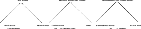

  

  (a) Quantity Wisdom ⊗ Quality Wisdom ⇒ Mind Wisdom (by Dai Ruwei) (b) Quantity Wisdom ⊗ Image Wisdom ⇒ Qualitative Wisdom (Mate Synthetic Wisdom) (by Hsue-shen Tsien) (c) Quantity Method ⊗ Fixation Image ⇒ Qualitative Method (Mate Synthetic Method (by Jiali Feng)

Based on the basic fact that the information received by human brain is, and only is the attributes of the objects, two basic hypothesis are proposed in this paper as follow:

Two Basic Hypothesis of Attribute Theory:

• (1) Human thinking can be constructed by some of processing attributes, such as, receiving, interpretation, and coding of attributes.

• (2) The mechanism of thinking construction and intelligent simulation can be considered as the mechanism of processing attribute.

If the two hypothesis are true, then we should study the following three basic questions:

• (1) What are the attributes?

• (2) How is an attribute and its transformation received, deciphered, interpreted and coded by brain?

• (3) How can the operators of Human Brain be represented by Mathematics?

In philosophy, an attribute is defined to be as follow [6]:

Definition 1:

An attribute is an expressing quality of an object when an interaction between the object and another object is happening.

As well-known that the spatial-time position of object $u$ ${\text{z}}_{1} \left( {t,u} \right)$, is the attribute showing where $u$ existing, the distance $d\left( {z_{1} ,z_{2} } \right)$ between u and its contradiction v is the expressing relation distinguishing that u from v, based on the fact, the intrinsic quality $q_{v} \left( u \right)$ of $u$ distinguish from its contradicted object $v$ can be defined by the corresponding relation “$u \ne v\; \,{ \Leftrightarrow }\;{\text{z}}_{1} \left( {t,u} \right) \ne {\text{z}}_{2} \left( {t,v} \right)\;{ \Leftrightarrow }\; \,{\text{d}}\left( {{\text{z}}_{1} ,{\text{z}}_{2} } \right) \ne 0$”. Based on the mechanism of $d\left( {z_{1} ,z_{2} } \right)$ varies with time change $\Delta {\text{t}}$ was controlled by law of the law of unity of opposites about the contradictory movements, such that the philosophy question: “when the $d\left( {z_{1} ,z_{2} } \right)$ vary with time change $\Delta {\text{t}}$, whether the intrinsic quality $q_{v} \left( u \right)$ of object $u$ keeps itself or not?” can be transform into a physical problem.

By mean of three equivalent definition of distance $d\left( {z_{1} ,z_{2} } \right)$, the Polarization Vector $\gamma_{c}$, $\gamma_{d}$ and $\upgamma$ of Inner Product $z_{1} \cdot z_{2}$, Entangled Vector, Entangled Circle $\odot O$, Entangled Coordinates and Clifford Algebra and so on for describing physical move of u and v, can be induced.

It is shown that if $\frac{{z_{1} }}{{\left| {z_{1} } \right|}}$ and $\frac{{z_{2} }}{{\left| {z_{2} } \right|}}$ are commeasurable each other, then Inner Product $z_{1} \cdot z_{2}$ can be measured as an integer that can be decomposed a product of some of Prime Factors, and a module can be deduced. But if $\frac{{z_{1} }}{{\left| {z_{1} } \right|}}$ and $\frac{{z_{2} }}{{\left| {z_{2} } \right|}}$ are non-commeasurable each other, then a measure system which value of unity continuously variable like the Fourier Orthogonal Base is necessary for the measure of Inner Product, and the requirement of value of distance $d\left( {z_{1} ,z_{2} } \right)$ is an integer is the foundation for orbit quantization.

Let $\Delta t_{it} = t - i$ be the time change, $\Delta z(\Delta t_{it} ) = (\Delta x(\Delta t_{it} ),\Delta y(\Delta t_{it} ))$ the displacement of $u$ and $v$ vary with $\Delta t_{it}$, then ${\text{z}}_{\text{t}} \left( {u,v} \right) = \left( {x_{\text{t}} \left( u \right),y_{t} \left( v \right)} \right) = {\text{z}}_{\text{i}} \left( {u,v} \right) +\Delta z(\Delta t_{it} ) = (\Delta x(\Delta t_{it} ),\Delta y(\Delta t_{it} )),$ and a category E whose object collection is $\left[ {i,T} \right) \times [z_{i} ,z_{T} )$, the arrow collection is $\{ (\Delta t_{it} ,\Delta x_{it} ,\Delta y_{it} )\}$ can be constructed.

The mechanism that the quality $q_{v} \left( u \right)$ is maintaining the same, during the quantity varies with time change in its qualitative criterion, can be abstracted as the Qualitative Mapping $\tau (x_{t} ,\left[ {x_{\text{i}} ,x_{\text{T}} } \right))$ from a quantity into its corresponding quality, and the regulation of different quantity convert into different quality of new quality, can be represented by the Degree Function of Conversion $\eta \left( {x_{\text{t}} } \right)$, such that a Cartesian Closed Category can be gotten by $\tau (x_{t} ,\left[ {x_{\text{i}} ,x_{\text{T}} } \right))$ and $\eta \left( {x_{\text{t}} } \right)$. A subobject classifier can be induced by the mechanism of a quality is changing to a simple (or non-essential) quality, so an Attribute Topos can be achieved by them.

Because a Hilbert Space ${\mathcal{H}}$ can be expanded by the Family of Qualitative Mappings, such that not only the degree of conversion function can be represented by a linear combination of base, but also a Tensor Flow can be induced by a functor F from the Base of H to Base of H’ with the time stream. A Fixation Image Operator, and an approach for Image Thought has been presented, some of applications in Noetic Science and Intelligent Science are discussed.

2 Entanglement Vectors Induced by Polarization Identity of Inner Product of Both Vectors z ₁ and z ₂

Let Z be the plan determined by vectors $z_{1}$ and $z_{2}$, and $z_{1} = \left( {x_{1} ,y_{1} } \right)$ and $z_{2} = \left( {x_{2} ,y_{2} } \right)$, the distance is defined the square root of inner product $z_{1} \cdot z_{2}$ of $z_{1}$ and $z_{2}$

$$ d\left( {z_{1} ,z_{2} } \right) = \sqrt {z_{1} \cdot z_{2} } = \sqrt {(x_{2} - x_{1} )^{2} + (y_{2} - y_{1} )^{2} } = \left| {z_{1} } \right|\left| {z_{2} } \right|cos\theta $$

(1)

But there is a Polarization Identity of inner product $z_{1} \cdot z_{2}$

$$ z_{1} \cdot z_{2} = \left( {\frac{{z_{1} + z_{2} }}{2}} \right)^{2} - \left( {\frac{{z_{1} - z_{2} }}{2}} \right)^{2} = \left( {\frac{{z_{1} }}{2} + \frac{{z_{2} }}{2}} \right)^{2} - \left( {\frac{{z_{1} }}{2} - \frac{{z_{2} }}{2}} \right)^{2} = \left( {\frac{{z_{1} }}{2} + \frac{{z_{1} }}{2}} \right)\left( {\frac{{z_{2} }}{2} + \frac{{z_{2} }}{2}} \right) $$

(2)

If let ${\text{A}} = {\text{A}}\left( {\frac{{x_{1} + x_{2} }}{4},\frac{{y_{1} + y_{2} }}{4}} \right)$, ${\text{B}} = {\text{B}}\left( {\frac{{x_{1} + x_{2} }}{2},\frac{{y_{1} + y_{2} }}{2}} \right)$, $\odot {\text{A}}$ the circle which diameter equal to $d_{{ \odot {\text{A}}}} = |OB|,$ $\odot {\text{B}}$ the circle which center is B, its radius equal to $r_{{ \odot {\text{B}}}} = \frac{{z_{1} - z_{2} }}{2}$. It is shown in Fig. 3(a) that there exist two Intersection Points of $\odot {\text{A}}$ and of $\odot {\text{B}}$, $C(c_{1} ,c_{2} )$ and $D(d_{1} ,d_{2} )$, their $c_{1}$ and $c_{2}$ are the horizontal coordinate of $C$ and the vertical coordinate of $C$, respectively, $d_{1}$ and $d_{2}$ of $D(d_{1} ,d_{2} )$ as well. Since $BC{ \bot }OC$, we have

Fig. 3.

(a) Polarization Circle $\odot O$ of Inner Product $z_{1} \cdot z_{2}$ (b) Entangled Coordinates

Fig. 4.

(a) Category induced by arrows $\{ \left( {\Delta t,\Delta x, \Delta y} \right)\}$ (b) Cone of arrows $F = \left\{ {\left( {a_{k} ,b_{k} ,c_{k} } \right)} \right\}$, (c) Pullback $\left( {a_{k} ,b_{k} } \right)$ of position mapping ($\varphi_{k}$, $\varphi_{k}$)

$$ \left\{ {\begin{array}{*{20}c} {{\text{OC}}^{2} = {\text{OB}}^{2} - {\text{BC}}^{2} = \left( {\frac{{z_{1} + z_{2} }}{2}} \right)^{2} - \left( {\frac{{z_{1} - z_{2} }}{2}} \right)^{2} = z_{1} \cdot z_{2} = \left| {z_{1} } \right|\left| {z_{2} } \right|cos\theta } \\ {{\text{OD}}^{2} = {\text{OB}}^{2} - {\text{BD}}^{2} = \left( {\frac{{z_{1} + z_{2} }}{2}} \right)^{2} - \left( {\frac{{z_{1} - z_{2} }}{2}} \right)^{2} = z_{1} \cdot z_{2} = \left| {z_{1} } \right|\left| {z_{2} } \right|cos\theta } \\ \end{array} } \right. $$

(3)

But $c_{1}$ and $c_{2}$ of $C(c_{1} ,c_{2} )$ are the solution of following two circles equations:

$$ \left\{ {\begin{array}{*{20}c} {\left( {c_{1} - \frac{{x_{1} + x_{2} }}{2}} \right)^{2} + \left( {c_{2} - \frac{{y_{1} + y_{2} }}{2}} \right)^{2} = \left( {\frac{{x_{2} - x_{1} }}{2}} \right)^{2} + \left( {\frac{{y_{2} - y_{1} }}{2}} \right)^{2} } \\ {\left( {c_{1} - \frac{{x_{1} + x_{2} }}{4}} \right)^{2} + \left( {c_{2} - \frac{{y_{1} + y_{2} }}{4}} \right)^{2} = \left( {\frac{{x_{2} - x_{1} }}{4}} \right)^{2} + \left( {\frac{{y_{2} - y_{1} }}{4}} \right)^{2} } \\ \end{array} } \right. $$

(4)

And the equation of chord $CD$ is the follow

$$ c_{1} = \frac{{2(x_{1} x_{2} + y_{1} y_{2} ) - c_{2} \left( {y_{2} + y_{1} } \right)}}{{x_{1} + x_{2} }} $$

(5)

By substituting (5) in (4), we get the solution of (4) as follow

$$ \left\{ \begin{aligned} c_{1} = \frac{{2(x_{1} + x_{2} )(x_{1} x_{2} + y_{1} y_{2} )\text{ + }(y_{1} + y_{2} )\sqrt {(x_{1} x_{2} + y_{1} y_{2} )[(x_{2} - x_{1} )^{2} + (y_{2} - y_{1} )^{2} ]} }}{{(x_{1} + x_{2} )^{2} + (y_{1} + y_{2} )^{2} }} \hfill \\ c_{2} = \frac{{2(x_{1} + x_{2} )(x_{1} x_{2} + y_{1} y_{2} ) - (x_{1} + x_{2} )\sqrt {(x_{1} x_{2} + y_{1} y_{2} )[(x_{2} - x_{1} )^{2} + (y_{2} - y_{1} )^{2} ]} }}{{(x_{1} + x_{2} )^{2} + (y_{2} + y_{1} )^{2} }} \hfill \\ \end{aligned} \right. $$

(6)

$$ \left\{ \begin{aligned} d_{1} = \frac{{2(x_{1} + x_{2} )(x_{1} x_{2} + y_{1} y_{2} ) - (y_{1} + y_{2} )\sqrt {(x_{1} x_{2} + y_{1} y_{2} )[(x_{2} - x_{1} )^{2} + (y_{2} - y_{1} )^{2} ]} }}{{(x_{1} + x_{2} )^{2} + (y_{1} + y_{2} )^{2} }} \hfill \\ d_{2} = \frac{{2(x_{1} + x_{2} )(x_{1} x_{2} + y_{1} y_{2} )\text{ + }(x_{1} + x_{2} )\sqrt {(x_{1} x_{2} + y_{1} y_{2} )[(x_{2} - x_{1} )^{2} + (y_{2} - y_{1} )^{2} ]} }}{{(x_{1} + x_{2} )^{2} + (y_{2} + y_{1} )^{2} }} \hfill \\ \end{aligned} \right. $$

(7)

Let $\odot O$ be the Circle whose center is the origin $O\left( {0,0} \right)$, its radius $r_{{ \odot {\text{O}}}} = \left| \gamma \right|$, $\left|\upgamma \right| = \left| {\upgamma_{c} } \right| = \sqrt {c_{1}^{2} + c_{2}^{2} } = \sqrt {d_{1}^{2} + d_{2}^{2} } = \left| {\upgamma_{d} } \right|$, then a Polar Coordinates $W\left( {\gamma ,\varphi } \right)$ can be induced by Polarization Identity, such that the points $C\left( {c_{1} ,c_{1} } \right)$ and $D\left( {d_{1} ,d_{1} } \right)$ can be written as two vectors $w_{c} \left( {\upgamma,\varphi_{c} } \right)$ and $w_{d} \left( {\upgamma,\varphi_{d} } \right)$ satisfying the follow

$$ \left\{ {\begin{array}{*{20}c} {C\left( {c_{1} ,c_{1} } \right) = w_{c} \left( {\upgamma,\varphi_{c} } \right) = {\upgamma }e^{{i\varphi_{c} }} =\upgamma\,\cos \varphi_{c} + i\upgamma\,\sin \varphi_{c} } \\ {D\left( {d_{1} ,d_{1} } \right) = w_{d} \left( {\upgamma,\varphi_{d} } \right) = {\upgamma }e^{{i\varphi_{d} }} =\upgamma\,\cos \varphi_{d} + i\upgamma\,\sin \varphi_{d} } \\ \end{array} } \right. $$

(8)

From the view of mathematical point, a Coordinates Transformation from product $Z \times Z$ to $W$-Plan has been constructed by (6), (7) and (8), $w:Z \times Z \to W$, for any $d_{ij} \left( {z_{i} \left( {x_{i} ,y_{i} } \right),z_{j} \left( {x_{j} ,y_{j} } \right)} \right)\,{ \in }\,Z \times Z$, such that

$$ w\left( {d_{ij} \left( {z_{i} \left( {x_{i} ,y_{i} } \right),z_{j} \left( {x_{j} ,y_{j} } \right)} \right)} \right) = w\left( {\upgamma,\varphi } \right)\left\{ {\begin{array}{*{20}l} {\begin{array}{*{20}l} {\begin{array}{*{20}l} {\upgamma^{2} = z_{1} \cdot z_{2} = \left| {z_{1} } \right|\left| {z_{2} } \right|cos\theta } \hfill \\ \end{array} } \hfill \\ {\varphi = \left\{ {\begin{array}{*{20}l} {arctg\frac{{c_{2} }}{{c_{1} }} \;or} \hfill \\ {arctg\frac{{d_{2} }}{{d_{1} }}} \hfill \\ \end{array} } \right.} \hfill \\ \end{array} } \hfill \\ \end{array} } \right. $$

(9)

(9) show us that both polarization vectors $w_{c} \left( {\upgamma,\varphi_{c} } \right)$ and $w_{d} \left( {\upgamma,\varphi_{d} } \right)$ is entangled together each other by identity: $\upgamma^{2} =\upgamma_{c}^{2} =\upgamma_{d}^{2}$ among $\upgamma_{c}$, $\upgamma_{d}$ and $d_{ij} \left( {z_{i} \left( {x_{i} ,y_{i} } \right),z_{j} \left( {x_{j} ,y_{j} } \right)} \right)$.

Let $E\left( {\left| {\upgamma_{E} } \right|,\varphi_{E} } \right)$ be the projection of $z_{2}$ on vector $z_{1}$, $\left| {\upgamma_{E} } \right| = \left| {z_{2} } \right|cos\theta$, and $\varphi_{E} = \alpha$. ${\text{E}}^{{\prime }} \left( {\left| {\upgamma_{{F^{{\prime }} }} } \right|,\theta + \alpha } \right)$ the projection of $z_{1}$ on vector $z_{2}$, $\left| {\upgamma_{{E^{{\prime }} }} } \right| = \left| {z_{1} } \right|cos\theta$, $\varphi_{{E^{\prime}}} = \theta + \alpha$, as shown in Fig. 3(b), so we have $^{{}} \left| {z_{1} } \right|^{2} = \left| {o{\text{E}}^{{\prime }} } \right|^{2} + \left| {z_{1} {\text{E}}^{{\prime }} } \right|^{2}$, $\left| {z_{2} } \right|^{2} = \left| {o{\text{E}}} \right|^{2} + \left| {z_{2} {\text{E}}} \right|^{2}$, addition that $\left| {z_{1} - z_{2} } \right|^{2} = \left| {z_{1} } \right|^{2} + \left| {z_{2} } \right|^{2} - 2\left| {z_{1} } \right|\left| {z_{2} } \right|cos\theta ,$ then we have

$$ \left| {z_{1} - z_{2} } \right|^{2} = \left| {o{\text{E}}^{{\prime }} } \right|^{2} + \left| {z_{1} {\text{E}}^{{\prime }} } \right|^{2} + \left| {o{\text{E}}} \right|^{2} + \left| {z_{2} {\text{E}}} \right|^{2} - 2\left| {z_{1} } \right|\left| {z_{2} } \right|cos\theta $$

(10)

It is shown that between the pair contradicted object $u$ and $v$, there is not only a polarization relation $\upgamma^{2} =\upgamma_{c}^{2} =\upgamma_{d}^{2}$, but also there exist an entangled relation (10).

It is obvious to see that by using a coordinates transformation, the intersection of $\odot O$ and vector $z_{1} - z_{2}$, note by $z_{0} = x_{0} + iy_{0}$, can be regarded to be the Origin point of respectively, and $m_{{z_{0} }} = \frac{{m_{{z_{1} }} m_{{z_{2} }} }}{{m_{{z_{1} }} + m_{{z_{2} }} }}$, the mass at the Electric Dipole Point $z_{0}$, because $E$ and $E^{{\prime }}$ represent Force $f = \left| {z_{1} } \right|\left| {z_{2} } \right|cos\theta$ action on $m_{{z_{1} }}$ and $m_{{z_{2} }}$ respectively, such that the Oscillation of EDP $z_{0}$ not only could be described by the, and some of Entangled reaction between $u$ and $v$ can be revealed out too.

In other hands, if let $z_{0}$ be the Harmonic Oscillation with mass $m_{{z_{0} }}$, then the law of Oscillation of $u$ with mass $m_{{z_{0} }}$ can be represented in. In special, when the distance $d\left( {z_{1} ,z_{2} } \right) \le h_{pc}$, because we have not the unit for accurate measure position of $z_{0} \left( u \right)$, such that what the object $u$ is become an uncertain problem, but the entangled relation between $u$ and $v$ is existing stile there.

In fact, we show from Fig. 3(a) that because $S_{ \odot O} = \pi\upgamma^{2}$, we get $\upgamma^{2} = z_{1} \cdot z_{2} = \left| {z_{1} } \right|\left| {z_{2} } \right|cos\theta = \frac{{S_{ \odot O} }}{\pi }$. And Fig. 3(b) show us that since $\left| {\overline{{Ez_{2} }} } \right| = \left| {z_{1} } \right|\left| {z_{2} } \right|sin\theta$, the Exterior Product $z_{1} \wedge z_{2}$ can be got by $z_{1} \wedge z_{2} = \left| {z_{1} } \right|\left| {z_{2} } \right|sin\theta = \left| {z_{1} } \right|\left| {\overline{{Ez_{2} }} } \right|$, and the Geometric Product $z_{1} z_{2}$ can be defined by $z_{1} z_{2} = z_{1} \cdot z_{2} + z_{1} \wedge z_{2}$ too, so a Geometric Algebra or Clifford Algebra as well.

From above analysis for Fig. 3, we have shown some of conceals information of Entangled Vector in bottom. One will naturally to ask: what more hidings are there the Entangled Vector? In order to get the answer, let us discuss it in detail in following.

Let E be the intersection point of $\odot O$ and vector $z_{1}$, $E\left( {\left| {\upgamma_{E} } \right|,\varphi_{E} } \right)$ and $E\left( {\left| {\upgamma_{E} } \right|,\alpha } \right)$ the E’s W-Plan coordinate and Z-Plan coordinate, respectively, and $E\left( {\left| {\upgamma_{E} } \right|,\varphi_{E} } \right) = E\left( {\left| {\upgamma_{E} } \right|,\alpha } \right)$, then $\upgamma_{E} = \sqrt {z_{1} \cdot z_{2} } = \sqrt {\left| {z_{1} } \right|\left| {z_{2} } \right|cos\theta }$, and $\varphi_{E} = \alpha$. Let $E^{{\prime }}$ be the intersection point of $\odot O$ and vector $z_{2}$, its W-Plan coordinate and Z-Plan coordinate are $E^{{\prime }} \left( {\left| {\upgamma_{{E^{{\prime }} }} } \right|,\varphi_{{E^{{\prime }} }} } \right)$ and $E^{{\prime }} \left( {\left| {\upgamma_{E} } \right|,\alpha + \theta } \right)$, respectively, and $E^{{\prime }} \left( {\left| {\upgamma_{{E^{{\prime }} }} } \right|,\varphi_{{E^{{\prime }} }} } \right) = \left( {E^{{\prime }} \left| {\upgamma_{{E^{{\prime }} }} } \right|,\alpha + \theta } \right)$, then $\upgamma_{{E^{{\prime }} }} = \sqrt {z_{1} \cdot z_{2} } = \sqrt {\left| {z_{1} } \right|\left| {z_{2} } \right|cos\theta }$, and $\varphi_{{E^{{\prime }} }} = \alpha + \theta$.

Let F be the projection on vector $z_{1}$ of $z_{2}$, $F\left( {\left| {\upgamma_{F} } \right|,\varphi_{F} } \right)$, $\left| {\upgamma_{F} } \right| = \left| {z_{2} } \right|cos\theta$, and $\varphi_{F} = \alpha$. F’ the projection on vector $z_{2}$ of $z_{1}$, ${\text{F}}^{{\prime }} \left( {\left| {\upgamma_{{F^{{\prime }} }} } \right|,\theta + \alpha } \right)$, $\left| {\upgamma_{{F^{{\prime }} }} } \right| = \left| {z_{1} } \right|cos\theta$, $\varphi_{{F^{{\prime }} }} = \theta + \alpha$.

Let G be the intersection point of $\odot A$ and $x$-axis, its W-Plan coordinate and Z-Plan coordinate are $G\left( {\left| {\upgamma_{G} } \right|,0} \right)$ and $G\left( {\left| {\upgamma_{G} } \right|,\alpha = 0} \right)$, respectively, and $G\left( {\left| {\upgamma_{G} } \right|,\varphi_{G} } \right) = G\left( {\left| {\upgamma_{G} } \right|,\alpha } \right)$, $\varphi_{G} = \alpha$. $G^{{\prime }}$ be the intersection point of $\odot A$ and $y$-axis, its W-Plan coordinate and Z-Plan coordinate are $G^{{\prime }} \left( {\left| {\upgamma_{{G^{{\prime }} }} } \right|,\varphi_{{G^{{\prime }} }} = \frac{\pi }{2}} \right)$ and $G^{{\prime }} \left( {\left| {\upgamma_{{G^{{\prime }} }} } \right|,\frac{\pi }{2}} \right)$, respectively, and $G^{{\prime }} \left( {\left| {\upgamma_{{G^{{\prime }} }} } \right|,\varphi_{{G^{{\prime }} }} } \right)$, $\varphi_{{G{\prime }}} = \frac{\pi }{2}$. Since $\left| {z_{F} } \right| = \left| {z_{2} } \right|cos\theta$, we get the follow

$$ \left| {\upgamma_{E} } \right|^{2} = \left| {z_{1} } \right|\left| {z_{2} } \right|cos\theta = \left| {z_{F} } \right|\left| {z_{1} } \right| = z_{1} \cdot z_{2} $$

(11)

Similarly,

$$ \left| {\gamma_{{E^{{\prime }} }} } \right|^{2} = \left| {z_{1} } \right|\left| {z_{2} } \right|cos\theta = \left| {z_{{F^{{\prime }} }} } \right|\left| {z_{2} } \right| = z_{1} \cdot z_{2} $$

(12)

Then we get

$$ \left| {z_{F} } \right|\left| {z_{1} } \right| = \left| {z_{{F^{{\prime }} }} } \right|\left| {z_{2} } \right| $$

(13)

We know that $\left| {\frac{{z_{1} }}{{\left| {z_{1} } \right|}}} \right|$ and $\left| {\frac{{z_{2} }}{{\left| {z_{2} } \right|}}} \right|$ are the unit of vector $z_{1}$ and $z_{2}$, respectively, note by $\left| {\frac{{z_{1} }}{{\left| {z_{1} } \right|}}} \right| \triangleq 1_{{z_{1} }}$ and $\left| {\frac{{z_{2} }}{{\left| {z_{2} } \right|}}} \right| \triangleq 1_{{z_{2} }}$, then we have from (13) that the norm $\left| {z_{F} } \right|$ of $z_{F}$ in $1_{{z_{1} }}$ equal to the norm $\left| {z_{{F{\prime }}} } \right|$ of $z_{{F^{\prime}}}$ in $1_{{z_{2} }}$.

It is easy to see that because $\sqrt {\left| {z_{F} } \right|}$ possible are an integer number, a rational number or an irrational number, whether $\left| {z_{F} } \right|$ is commensurable by using the unit $1_{{z_{1} }}$? Become a key problem. For example, $\sqrt {\left| {z_{F} } \right|} = \sqrt 2$, because $\sqrt 2$ can’t be measured by using the unit $1_{{z_{1} }}$, such that $\left| {\upgamma_{E} } \right|$ can’t be described in precision.

In order to discuss simple, first of all, let Z-Plan and W-Plan rotate an angle $\theta$, such that the direct of vector $z_{1}$ turns into that of $x_{1}$, such that $1_{{z_{1} }} = 1_{{x_{1} }}$.

Second, assume $\sqrt {\left| {z_{F} } \right|}$ can be measured by $1_{{x_{1} }}$, then there exits an unit system: $\left\{ {\frac{{1_{{x_{1} }} }}{{m^{k} }} = 1_{{x_{1} }}^{k} ,k = 0, \ldots ,N} \right\}$, such that

$$ \left| {z_{F} } \right| = n_{0} 1_{{x_{1} }}^{0} + n_{1} 1_{{x_{1} }}^{1} + \ldots + n_{N} 1_{{x_{1} }}^{N} = \sum\nolimits_{k = 0}^{N} {n_{k} 1_{{x_{1} }}^{k} = n_{0} .n_{1} \ldots n_{N} } $$

(14)

Since $1_{{x_{1} }}^{k} = 1_{{x_{1} }}^{k - 1} \times m$, and $\frac{{1_{{x_{1} }} }}{{m^{N} }}$ is the minimum unit in this system, norm of $\left| {z_{F} } \right|$ can be written as follow:

$$ \left| {z_{F} } \right| = n_{0} .n_{1} \ldots \,n_{N} = n_{0} \times 1 + n_{1} \times m^{1} \ldots n_{N} \times m^{N} = n\quad ({\text{in}}\frac{{1_{{x_{1} }} }}{{m^{N} }} = 1) $$

(15)

In other hands, if there are s prime factor of $n$, $p_{l} ,l = 1, \ldots s$, such that $n = p_{1} \times p_{2} \times \ldots \times p_{s}$, then we get another unit system: $\left\{ {\frac{{1_{n} }}{{p_{l} }} = 1_{n}^{{p_{l} }} ,l = 0, \ldots ,s} \right\}$, such that

$$ \left| {z_{F} } \right| = n = (p_{0} \times \ldots \times p_{l - 1} \times \hat{p}_{l} \times p_{1 + 1} \times \ldots \times p_{s} )1_{n}^{{p_{l} }} $$

(16)

here, symbol $\hat{p}_{l}$ represents the lack of the prime factor $p_{l}$. It is mean from (15) that by using prime factor $p_{l}$ of $n$ as unit for the measurement of the norm of $\left| {z_{F} } \right|$, its value equal to $\left( {p_{0} \cdot p_{1} \cdot p_{l - 1} \cdot \hat{p}_{l} \cdot p_{1 + 1} \cdot p_{s} } \right)$. Therefore, prime factor $p_{l}$ can be called an eigenvector of $\left| {z_{F} } \right|$, and $\left( {p_{0} \cdot p_{1} \cdot p_{l - 1} \cdot \hat{p}_{l} \cdot p_{1 + 1} \cdot p_{s} } \right)$ is called the eigenvalues of the eigenvector $p_{l}$ of $\left| {z_{F} } \right|$.

If $\sqrt {\left| {z_{F} } \right|}$ is an infinite rational number, for instant 1/3, then

If $\sqrt {\left| {z_{F} } \right|}$ can’t be measured by $1_{{x_{1} }}$, then we need an unit system whose value of unit is continuously variable, otherwise, the norm of $\sqrt {\left| {z_{F} } \right|}$ can’t be measured.

We all know that

$$ \int_{0}^{x} {dt = t|_{0}^{x} = x} $$

(17)

Because $x$ is the norm of the interval $\left[ {0,x} \right]$, the solution of (17) enlightens us that integration (17) is just the measure for norm of the interval $\left[ {0,x} \right]$ using $dt$ as the unity (or rule) of measure. In other words, $dt$ can be considered to be the unit $1_{{x_{1} }}^{k}$, when $k \to \infty$, i.e. $dt = \mathop { \lim }\limits_{k \to \infty } 1_{{x_{1} }}^{k} = 1_{{x_{1} }}^{\infty }$.

In other hands, for the interval $\left[ {0,x} \right]$, we have that $x\left( t \right) = \left( {1 - t} \right)x_{0} + tx_{1}$, let $\Delta x = x - x_{0}$, then $t = \frac{{\Delta x}}{{x_{1} - x_{0} }}$, and $dx\left( t \right) = (x_{1} - x_{0} )dt$, so we have

$$ dt = \mathop {\lim }\nolimits_{\Delta x \to 0} \frac{{\Delta x}}{{x_{1} - x_{0} }} = \frac{dx}{{x_{1} - x_{0} }} $$

(18)

Integral for (18) we get

$$ \int_{0}^{{t_{E} }} {dt = \frac{1}{{x_{1} - x_{0} }}} \int_{{x_{0} }}^{{x_{E} }} {dx = \left. {\frac{x}{{x_{1} - x_{0} }}} \right|_{{x_{0} }}^{{x_{E} }} } = \frac{{x_{E} - x_{0} }}{{x_{1} - x_{0} }} = \left. {\frac{{x_{E} }}{{x_{1} }}} \right|_{{x_{0} = 0}}^{{x_{E} }} $$

(19)

Since $\left| {x_{1} } \right| = \left| {z_{1} } \right| = 1_{{z_{1} }}$, we have the follow:

$$ dt = \left. {\frac{dx}{{x_{1} - x_{0} }}} \right|_{{x_{0} = 0}}^{{x_{E} }} = \frac{dx}{{\left| {x_{1} } \right|}} = \frac{dx}{{\left| {z_{1} } \right|}} = \frac{dx}{{\left| {1_{{x_{1} }} } \right|}} $$

(20)

It is hiding from (18) and (19) that (20) could be assumed to being the minimum unit of measure.

Then we get

$$ \left| {x_{F} } \right|\int_{0}^{{t_{E} }} {dt = } \frac{{\left| {x_{F} } \right|}}{{\left| {x_{1} } \right|}}\int_{0}^{{x_{E} }} {dx = } \left. {\frac{{\left| {x_{F} } \right|}}{{\left| {x_{1} } \right|}}x} \right|_{0}^{{x_{E} }} = \frac{{\left| {x_{F} } \right|\left| {x_{E} } \right|}}{{\left| {x_{1} } \right|}}\;({\text{in}}\frac{{\left| {x_{F} } \right|dx}}{{\left| {1_{{x_{1} }} } \right|}} = 1) $$

(21)

Let $\Delta x\left( {\Delta t} \right) = \lambda t$ then $x_{t} = x_{0} +\Delta x\left( {\Delta t} \right) = x_{0} + \lambda t$,

$$ \varphi \left( {x_{t} } \right) = \int_{0}^{{t_{E} }} {x_{t} dt = } \int_{0}^{{x_{E} }} {\left( {x_{0} + \lambda t} \right)dx = } \left. {\left( {x_{0} t + \frac{{\lambda t^{2} }}{2}} \right)} \right|_{0}^{{x_{E} }} = \frac{{\lambda x_{E}^{2} }}{2} = \frac{{\lambda\upgamma^{2} }}{2} $$

(22)

Let $\Delta y\left( {\Delta t} \right) = - i\lambda t$ then $y_{t} = y_{0} +\Delta y\left( {\Delta t} \right) = y_{0} - i\lambda t$,

$$ \phi \left( {y_{t} } \right) = \int_{0}^{{t_{{E^{{\prime }} }} }} {y_{t} dt = } \int_{0}^{{y_{E} }} {\left( {y_{0} - i\lambda t} \right)} dx = \left. {\left( {y_{0} t - i\frac{{\lambda t^{2} }}{2}} \right)} \right|_{0}^{{y_{{E^{{\prime }} }} }} = - \frac{{i\lambda y_{{E^{{\prime }} }}^{2} }}{2} = - \frac{{i\lambda^{2} }}{2} $$

(23)

Let $\Delta z\left( {\Delta t} \right) = \lambda \left( {1 - i} \right)t$ and $z_{t} = z_{0} +\Delta z\left( {\Delta t} \right) = \left( {x_{0} + iy_{0} } \right) + \lambda \left( {1 - i} \right)t$

Then we get

$$ U\left( {z_{t} } \right) = \varphi \left( {x_{t} } \right) + i\phi \left( {y_{t} } \right) = \frac{{\lambda x_{E}^{2} }}{2} + i\left( { - \frac{{i\lambda y_{{E^{{\prime }} }}^{2} }}{2}} \right) = \frac{\lambda }{2}\left( {x_{E}^{2} + y_{{E^{{\prime }} }}^{2} } \right) = \lambda\upgamma^{2} $$

(24)

$$ U\left( {z_{t} } \right) = \varphi \left( {z_{t} } \right) + i\phi \left( {z_{t} } \right) = \varphi \left( {x_{0} + \lambda t} \right) + i\phi \left( {y_{0} - i\lambda t} \right) = \lambda^{2}\upgamma^{2} $$

(25)

Then we have a wave equation:

$$ \frac{{d^{2} U}}{{dt^{2} }} - \frac{1}{{\lambda^{2} }}\frac{{d^{2} U}}{{dz^{2} }} = 0 $$

(26)

It is shown from above discuss that object $u$ and $v$ are entangled each other by (25). If $\Delta t < t_{pl}$, $t_{pl}$ is Planck Time, the entangled relation (25) between $u$ and $v$ will be remained yet, then it could be called the quantum entanglement. An encryption and decryption algorithm based on the entangled vector $\upgamma_{c}$ and $\upgamma_{d}$ of $z_{1}$ and $z_{2}$, has been proposed by Jiali Feng [7]. The encryption and decryption algorithm based quantum entanglement among $\upgamma_{c}$,$\upgamma_{d}$ and $\gamma$ would be discussed in other paper.

3 The Attribute Topos Induced by Mechanism of Mutual Change Between Quality and Quantity

Because the position changes with time $\Delta t_{it}$, $\Delta z(\Delta t_{it} ) = (\Delta x(\Delta t_{it} ),\Delta y(\Delta t_{it} ))$ induces a cone and a limit among arrows $\{ (\Delta t_{it} ,\Delta x_{it} ),\Delta y_{it} )\}$, as shown in Figs. 5, 6 and 7, such that a finitely complete category can be achieved.

Fig. 5.

(a) the Cartesian Closed Category induced by function $f\left( {x_{t} ,x_{k} } \right)$ and $\tau_{i} \left( {x_{k} } \right)$ (b) Quality change $\tau_{i}^{j} \left( x \right) = \left\{ {\begin{array}{*{20}c} { + 1} \\ { - 1} \\ \end{array} } \right.$ of $\tau_{j} \left( x \right) - \tau_{i} \left( x \right)$ and its Harr wavelet (c) Pullback induced by Qualitative Mapping $\tau_{\varphi } \left( {x_{t} ,\left[ {x_{i} ,\left. {x_{T} } \right)} \right.} \right)$

Fig. 6.

(a) “Fixation-Image” operator of EGR. (b) Recognition algorithm of EGR based on Qualitative Mapping

Fig. 7.

Human face recognition based on qualitative mapping

Let $\left[ {i,T} \right)$ and $\left[ {x_{\text{i}} ,x_{\text{T}} } \right)$ be the time interval and position interval in which $q_{v} \left( u \right)$ maintains itself, then $q_{v} \left( u \right)$ must be fixed, as long as $x_{\text{t}} = x_{\text{t}} +\Delta x(\Delta t_{it} )$ of $u$ does not over out $\left[ {x_{\text{i}} ,x_{\text{T}} } \right)$, i.e. $x_{\text{t}} \,{ \in }\,\left[ {x_{\text{i}} ,x_{\text{T}} } \right)$, while the displacement $\Delta x(\Delta t_{it} )$ vary with $\Delta t_{it}$. It is obvious that the mechanism of the conversion from quantity $x_{\text{t}}$ into a quality $q_{v} \left( u \right)$ can be described by a Qualitative Mapping as follow

$$ \tau (x_{t} ,\left[ {x_{0} ,x_{\text{T}} } \right)) = \left\{ {\begin{array}{*{20}c} {q_{v} \left( u \right)\quad \quad \quad x_{t} \,{ \in }\, \left[ {x_{\text{i}} ,x_{\text{T}} } \right)} \\ {{\neg }q_{v} \left( u \right)\quad \quad \quad x_{t} \,{ \in }\, \left[ {t_{0} ,t_{i} } \right] } \\ \end{array} } \right. $$

(27)

Let $x_{\text{t}} ,x_{\text{s}} \,{ \in }\,\left[ {x_{\text{i}} ,x_{\text{T}} } \right)$ be two quantities belonging to a same qualitative criterion $\left[ {x_{\text{i}} ,x_{\text{T}} } \right)$, even they are conversing into the same quality $q_{v} \left( u \right)$, their degrees of conversion are different. To describe this case, a function of conversion degree $\eta \left( {x_{\text{t}} ,\left[ {x_{\text{i}} ,x_{\text{T}} } \right)} \right) = \eta \left( {x_{\text{t}} } \right)$ has been proposed by Attribute Theory. In other words, let $\left[ {i,T} \right) \times [x_{i} ,x_{T} )$ be the product of $\left[ {i,T} \right)$ and $[x_{i} ,x_{T} )$, $\left[ {y_{\text{i}} ,y_{\text{T}} } \right)$ codomain of $\eta \left( {x_{\text{t}} } \right)$, we get the follow

$$ \eta{:}\,\left[ {i,T} \right) \times [x_{i} ,x_{T} ) \to \left[ {\eta_{\text{i}} ,\eta_{\text{T}} } \right) $$

(28)

It is obvious that there is an equivalent relation, between the function of conversion degree $\eta{:}\,\left[ {i,T} \right) \times [x_{i} ,x_{T} ) \to \left[ {\eta_{\text{i}} ,\eta_{\text{T}} } \right)$ and the $\eta^{{\prime }}{:}\,\left[ {i,T} \right) \to [x_{i} ,x_{T} ) \times \left[ {\eta_{\text{i}} ,\eta_{\text{T}} } \right)$, this is said that in category

$$ \hom \left( {\left[ {i,T} \right) \times [x_{i} ,x_{T} } \right),\left[ {\eta_{\text{i}} ,\eta_{\text{T}} } \right)) \approx { \hom }\left( {\left[ {i,T} \right),[x_{i} ,x_{T} } \right) \times \left[ {\eta_{\text{i}} ,\eta_{\text{T}} } \right)) $$

(29)

Therefore, we get a Cartesian Closed Category induced by the function $\eta \left( {t,\left[ {{\text{x}}_{\text{i}} ,{\text{x}}_{\text{T}} } \right)} \right)$ and $\uptau_{\text{i}} \left( {x_{k} ,\left[ {{\text{x}}_{\text{i}} ,{\text{x}}_{\text{T}} } \right)} \right)$. In other words, there is an evaluation morphism induced by $\eta \left( {t,\left[ {{\text{x}}_{0} ,{\text{x}}_{\text{T}} } \right)} \right)$ and $\uptau_{\text{i}} \left( {x_{k} ,\left[ {{\text{x}}_{\text{i}} ,{\text{x}}_{\text{T}} } \right)} \right)$, ${\text{ev}}{:}\,\left[ {i,T} \right) \times \left[ {\eta_{\text{i}} ,\eta_{\text{T}} } \right)^{{\left[ {i,T} \right)}} \to \left[ {\eta_{\text{i}} ,\eta_{\text{T}} } \right)$, such that ${\text{ev}}\left( {t,\uptau_{\text{i}} \left( {x_{k} } \right)} \right) =\uptau\left( {x_{k} } \right)\left( t \right) = \eta \left( {t,x_{k} } \right)$, here the exponential morphism is $\uptau_{\text{i}} \left( {{\text{x}}_{\text{k}} ,\left[ {{\text{x}}_{\text{i}} ,{\text{x}}_{\text{T}} } \right)} \right)$, as shown in Fig. 5(a) [8].

If let $x_{\text{j}} \,{ \in }\,\left[ {x_{\text{j}} ,x_{j + l} } \right)\,{ \subseteq }\,\left[ {x_{\text{i}} ,x_{\text{T}} } \right)$ be the point that quality $q_{v} \left( u \right)$ transform to its non-essential quality $q_{j} \left( u \right)$, note by “$q_{v} \to q_{j}$” or $q_{v}^{j}$, $\left[ {x_{\text{j}} ,x_{j + l} } \right)$ the qualitative criterion of $q_{j} \left( u \right)$, in which $q_{j} \left( u \right)$ will remain itself, as long as $x_{\text{t}}$ varies with time change $\Delta t_{it}$ but still in $\left[ {x_{\text{j}} ,x_{j + l} } \right)$, and let $x_{\text{T}} \in \left( {x_{{{\text{T}}^{ - } }} ,x_{{{\text{T}}^{ + } }} } \right)$ be the point at that the quality $q_{v} \left( u \right)$ transform to the quality $p_{u} \left( v \right)$ of $v$, the contradiction of $u$, or when the distance $\left| {\left( {x_{{{\text{T}}^{ - } }} ,x_{{{\text{T}}^{ + } }} } \right)} \right| \le h_{pl}$, the Planck constant, a system $S_{{\left( {u,v} \right)}}$ can be constructed by $u$ and $v$, i.e. $x_{\text{t}} \,{ \notin }\,\left[ {x_{\text{i}} ,x_{\text{T}} } \right), x_{\text{t}} \,{ \in }\,\left( {x_{{{\text{T}}^{ - } }} ,x_{{{\text{T}}^{ + } }} } \right) \wedge \left| {\left( {x_{{{\text{T}}^{ - } }} ,x_{{{\text{T}}^{ + } }} } \right)} \right| \le h_{pl}$. Then we have a Qualitative Mapping as following

$$ \tau (x_{t} ,[x_{0} ,x_{\text{T}} )) = \left\{ {\begin{array}{*{20}l} {S_{(u,v)} } \hfill & {x_{\text{t}} \in [x_{\text{T}} ,x_{{{\text{T}}^{ + } }} ] \wedge \left| {[x_{\text{T}} ,x_{{{\text{T}}^{ + } }} ]} \right| \le h_{pl} } \hfill \\ {p_{u} (v)} \hfill & {x_{t} = [x_{{{\text{T}}^{ - } }} ,x_{\text{T}} ]} \hfill \\ {q_{j} (u)} \hfill & {x_{t} \in [x_{\text{j}} ,x_{j + l} )} \hfill \\ {q_{v} (u)} \hfill & {x_{t} \in [x_{\text{i}} ,x_{\text{T}} )} \hfill \\ {\neg q_{v} (u)} \hfill & {x_{t} \in \left[ {t_{\text{0}} ,t_{i} } \right]} \hfill \\ \end{array} } \right. $$

(30)

The mechanism of a non-essential transforms from the quality $q_{i} \left( u \right)$ to its sub-quality ${\text{q}}_{\text{j}} \left( {\text{u}} \right)$, notation as

$$ \uptau_{i}^{j} \left( x \right) =\uptau_{\text{j}} \left( {x,\left[ {x_{\text{j}} ,x_{\text{T}} } \right)} \right) -\uptau_{i} \left( {x,\left[ {x_{i} ,x_{\text{j}} } \right)} \right) = \left\{ {\begin{array}{*{20}c} {0_{j} - 1_{i} = - 1_{i}^{j} \quad x\,{ \in }\,[x_{i} ,x_{\text{j}} )} \\ {1_{j} - 0_{i} = 1_{i}^{j} \quad x\,{ \in }\,\left[ {x_{\text{j}} ,x_{\text{T}} } \right)} \\ \end{array} } \right. $$

(31)

The (15) show that a Harr wavelet induced by the difference of $\uptau_{\text{j}} \left( {x,\left[ {x_{\text{j}} ,x_{\text{T}} } \right)} \right) -\uptau_{i} \left( {x,\left[ {x_{i} ,x_{\text{j}} } \right)} \right)$ or $\uptau_{i}^{j} \left( x \right)$, when $[x_{i} ,x_{\text{j}} ),\left[ {x_{\text{j}} ,x_{\text{T}} } \right)\,{ \subseteq }\,\left[ {{\text{x}}_{\text{i}} ,{\text{x}}_{\text{T}} } \right)$, and $[x_{i} ,x_{\text{j}} )\,{ \cap }\,\left[ {x_{\text{j}} ,x_{\text{T}} } \right) = {\emptyset }$.

Let $\upvarphi :\left[ {{\text{x}}_{\text{i}} ,\left.{{\text{x}}_{\text{j}} } \right)} \right. \hookrightarrow \left[ {{\text{x}}_{0} ,\left. {{\text{x}}_{\text{T}} } \right)} \right.$ be the monic function induced by the inclusion relation $\left[ {{\text{x}}_{\text{i}} ,{\text{x}}_{\text{j}} } \right)\,{ \subseteq }\,\left[ {{\text{x}}_{0} ,{\text{x}}_{\text{T}} } \right)$, the characteristic function $\uptau_{{\varphi }} \left( {{\text{x}}_{\text{t}} ,\left[ {{\text{x}}_{\text{i}} ,\left. {{\text{x}}_{\text{j}} } \right)} \right.} \right)$ induced by ${\varphi }$ is just the qualitative mapping which criterion is $\left[ {{\text{x}}_{\text{i}} ,\left. {{\text{x}}_{\text{T}} } \right)} \right.$. This means that, not only a truth map true: $\left\{ 0 \right\} \to\Omega = \left\{ {0,1} \right\}$, but also a pullback square as shown in Fig. 4 can be induced by $\uptau_{{\varphi }} \left( {{\text{x}}_{\text{t}} ,\left[ {{\text{x}}_{\text{i}} ,\left. {{\text{x}}_{\text{T}} } \right)} \right.} \right)$. In particular, if $\uppsi:\left[ {{\text{x}}_{\text{j}} ,\left. {{\text{x}}_{\text{T}} } \right)} \right. \hookrightarrow \left[ {{\text{x}}_{0} ,\left. {{\text{x}}_{\text{T}} } \right)} \right.$ is a monic morphism induced by the relation $\left[ {{\text{x}}_{\text{j}} ,\left. {{\text{x}}_{\text{T}} } \right)} \right.\, \subseteq \,\left[ {{\text{x}}_{0} ,\left. {{\text{x}}_{\text{T}} } \right)} \right.$, such that $\uppsi\left( {{\text{x}}_{\text{k}} } \right)\, \in \,\left[ {{\text{x}}_{0} ,\left. {{\text{x}}_{\text{T}} } \right)} \right.$, then there exists a function induced by $\uppsi\upphi :\left[ {{\text{x}}_{\text{j}} ,\left. {{\text{x}}_{\text{T}} } \right)} \right. \hookrightarrow \left[ {{\text{x}}_{\text{i}} ,\left. {{\text{x}}_{\text{T}} } \right)} \right.$, for ${\forall }{\text{x}}_{\text{k}} \,{ \in }\,\left[ {{\text{x}}_{\text{j}} ,\left. {{\text{x}}_{\text{T}} } \right)} \right.$, $\upphi\left( {{\text{x}}_{\text{k}} } \right)\,{ \in }\,\left[ {{\text{x}}_{\text{i}} ,\left. {{\text{x}}_{\text{T}} } \right)} \right.$, such that ${\upvarphi \circ \upphi }\left( {{\text{x}}_{\text{k}} } \right) = {\upvarphi }\left( {{\text{x}}_{\ell } } \right) = {\uppsi }\left( {{\text{x}}_{\text{k}} } \right)$.

In other word, because 1 = {0}, and there is the inclusion mapping $1 = \left\{ 0 \right\}\, \subseteq \,\left\{ {0,1} \right\}$, for any subset $\left[ {{\text{x}}_{\text{j}} ,\left. {{\text{x}}_{\text{T}} } \right)} \right.\,{ \subseteq }\,\left[ {{\text{x}}_{0} ,\left. {{\text{x}}_{\text{T}} } \right)} \right.$ and the morphism $\left[ {{\text{x}}_{\text{j}} ,\left. {{\text{x}}_{\text{T}} } \right)} \right. \to 1$, the pullback square can be gotten, but any subset $\left[ {{\text{x}}_{\text{j}} ,\left. {{\text{x}}_{\text{T}} } \right)} \right.\,{ \subseteq }\,\left[ {{\text{x}}_{0} ,\left. {{\text{x}}_{\text{T}} } \right)} \right.$ is true, if and only if, $\uptau_{\upphi} \left( {{\text{x}}_{\text{k}} ,\left[ {{\text{x}}_{\text{j}} ,\left. {{\text{x}}_{\text{T}} } \right)} \right.} \right) = 1$. This means that there is only one predication “for ${\forall }{\text{x}}_{\text{k}} \,{ \in }\,\left[ {{\text{x}}_{\text{j}} ,\left. {{\text{x}}_{\text{T}} } \right)} \right.\,{ \subseteq }\,\left[ {{\text{x}}_{0} ,\left. {{\text{x}}_{\text{T}} } \right)} \right.$, the true mapping $\left[ {{\text{x}}_{\text{j}} ,\left. {{\text{x}}_{\text{T}} } \right)} \right. \to 1 \to\Omega$”, and $\Omega$ is a subobject classifier. Therefore, we get an Attribute Topos.

4 The Fixation Image Operator Induced by Orthogonal Expanded of Function

Let $\left[ {{\text{x}}_{\text{i}} ,{\text{x}}_{\text{T}} } \right) = \bigcup\nolimits_{{{\text{k}} = 1}}^{\text{m}} {\left[ {{\text{x}}_{\text{i}} ,{\text{x}}_{{{\text{i}} + {\text{k}}}} } \right)}$, we get a collection of qualitative mapping $\left\{ {\uptau_{\text{j}} \left( {{\text{x}}_{\text{k}} ,\left[ {{\text{x}}_{\text{j}} ,{\text{x}}_{{{\text{j}} + 1}} } \right)} \right),{\text{j}} = {\text{i}},{\text{i}} + 1, \ldots ,{\text{i}} + {\text{m}},} \right\}$, and for ${\forall \tau }_{{{\text{j}}_{1} }} \left( {{\text{x}}_{\ell } ,\left[ {{\text{x}}_{{{\text{j}}_{1} }} ,{\text{x}}_{{{\text{j}}_{1} + 1}} } \right)} \right),\uptau_{{{\text{j}}_{2} }} \left( {{\text{x}}_{\text{k}} ,\left[ {{\text{x}}_{{{\text{j}}_{2} }} ,{\text{x}}_{{{\text{j}}_{2} + 1}} } \right)} \right)\;{ \in }\left\{ {\uptau_{\text{j}} \left( {{\text{x}}_{\text{k}} ,\left[ {{\text{x}}_{\text{j}} ,{\text{x}}_{{{\text{j}} + 1}} } \right)} \right)} \right\}$, ${\exists }{\text{x}}_{\ell } \,{ \in }\,\left[ {{\text{x}}_{{{\text{j}}_{1} }} ,{\text{x}}_{{{\text{j}}_{1} + 1}} } \right)$, for ${\forall }{\text{x}}_{\text{k}} \,{ \in }\,\left[ {{\text{x}}_{{{\text{j}}_{2} }} ,{\text{x}}_{{{\text{j}}_{2} + 1}} } \right)$, their inner product satisfying the following

$$ \int_{{{\text{j}}_{2} }}^{{{\text{j}}_{2 + 1} }} {\uptau_{{{\text{j}}_{1} }} \left( {{\text{x}}_{\ell } ,\left[ {{\text{x}}_{{{\text{j}}_{1} }} ,{\text{x}}_{{{\text{j}}_{1} + 1}} } \right)} \right)\uptau_{{{\text{j}}_{2} }} \left( {{\text{x}}_{\text{k}} ,\left[ {{\text{x}}_{{{\text{j}}_{2} }} ,{\text{x}}_{{{\text{j}}_{2} + 1}} } \right)} \right){\text{dx}}_{\text{k}} = \left\{ {\begin{array}{*{20}c} {1\quad \quad {\text{j}}_{1} = {\text{j}}_{2} } \\ {0\quad \quad {\text{j}}_{1} \ne {\text{j}}_{2} } \\ \end{array} } \right.} $$

(32)

This shows that not only the collection $\left\{ {\uptau_{\text{j}} \left( {{\text{x}}_{\text{k}} ,\left[ {{\text{x}}_{\text{j}} ,{\text{x}}_{{{\text{j}} + 1}} } \right)} \right)} \right\}$ constructs an orthogonal base and by which a Hilbert Space ${\mathcal{H}}$ can be expanded, but also any function of conversion degree ${\text{f}}\left( {{\text{x}}_{\text{t}} ,\left[ {{\text{x}}_{\text{i}} ,{\text{x}}_{\text{T}} } \right)} \right)$ can be expanded into a linear combination of qualitative mappings as follow

$$ {\text{f}}\left( {{\text{x}}_{\text{t}} ,\left[ {{\text{x}}_{\text{i}} ,{\text{x}}_{\text{T}} } \right)} \right) = \sum\nolimits_{{{\text{k}} = 1}}^{\text{m}} {{\text{f}}_{\text{k}} \left( {{\text{x}}_{\text{t}} ,\left[ {{\text{x}}_{\text{i}} ,{\text{x}}_{{{\text{i}} + {\text{k}}}} } \right)} \right)\uptau_{\text{j}} \left( {{\text{x}}_{\text{k}} ,\left[ {{\text{x}}_{\text{i}} ,{\text{x}}_{{{\text{i}} + {\text{k}}}} } \right)} \right)} $$

(33)

In fact, because a generalized Fourier Transformation of ${\text{f}}\left( {{\text{x}}_{\text{t}} ,\left[ {{\text{x}}_{\text{i}} ,{\text{x}}_{\text{T}} } \right)} \right){\text{F}}\left( {\text{f}} \right)$ can be defined by the inner product of ${\text{f}}\left( {{\text{x}}_{\text{t}} ,\left[ {{\text{x}}_{\text{i}} ,{\text{x}}_{\text{T}} } \right)} \right)$ and $\uptau_{\text{i}} \left( {{\text{x}}_{\ell } ,\left[ {{\text{x}}_{\text{j}} ,{\text{x}}_{{{\text{j}} + {\text{w}}}} } \right)} \right)$ as following:

$$ {\text{F}}\left( {\text{f}} \right) = \left( {{\text{f}}\left( {{\text{x}}_{\text{t}} ,\left[ {{\text{x}}_{\text{i}} ,{\text{x}}_{\text{T}} } \right)} \right),\uptau_{\text{i}} \left( {{\text{x}}_{\ell } ,\left[ {{\text{x}}_{\text{j}} ,{\text{x}}_{{{\text{j}} + {\text{w}}}} } \right)} \right)} \right) = \left\{ {\begin{array}{*{20}l} {{\text{f}}_{\text{k}} \left( {{\text{x}}_{\text{t}} ,\left[ {{\text{x}}_{\text{i}} ,{\text{x}}_{{{\text{i}} + {\text{k}}}} } \right)} \right)} \hfill & {\text{i = j}} \hfill \\ 0 \hfill & {{\text{i}} \ne {\text{j}}} \hfill \\ \end{array} } \right. $$

(34)

By (34) the degree of conversion function ${\text{f}}\left( {{\text{x}}_{\text{t}} ,\left[ {{\text{x}}_{\text{i}} ,{\text{x}}_{\text{T}} } \right)} \right)$ could be homomorphically (or similarly) mapped from the function space into a vector or the point $({\text{f}}_{1} \left( {{\text{x}}_{\text{t}} ,\left[ {{\text{x}}_{{{\text{i}} + 1}} ,{\text{x}}_{{{\text{i}} + 2}} } \right)} \right), \ldots , {\text{f}}_{\text{m}} \left( {{\text{x}}_{\text{t}} ,\left[ {{\text{x}}_{{{\text{i}} + \left( {{\text{m}} - 1} \right)}} ,{\text{x}}_{{{\text{i}} + {\text{m}}}} } \right)} \right)$ in the Hilbert space ${\mathcal{H}}$, so (34) is called the “Fixation-Image” operator of function ${\text{f}}\left( {{\text{x}}_{\text{t}} ,\left[ {{\text{x}}_{\text{i}} ,{\text{x}}_{\text{T}} } \right)} \right)$.

In other words, this shows that a Hilbert Space ${\mathcal{H} }$ is expanded by an Orthogonal Base $\left\{ {\uptau_{\text{j}} \left( {{\text{x}}_{\text{k}} ,\left[ {{\text{x}}_{\text{j}} ,{\text{x}}_{{{\text{j}} + 1}} } \right)} \right)} \right\}$ which is induced by the Subobject Classifier of Attribute Topos. In the next, let us discuss its application.

Let $\left\{ {{\text{f}}^{\text{s}} } \right\}$ be the collection of the approximation ${\text{f}}^{\text{s}}$ of function ${\text{f}}$, ${\text{F}}$ the “Fixation Image” operator ${\text{F}}:\left\{ {{\text{f}}^{\text{s}} } \right\} \to {\mathcal{H}}$, ${\text{F}}\left( {\left\{ {{\text{f}}^{\text{s}} } \right\}} \right) = {\text{N}}\left( {{\text{F}}\left( {\text{f}} \right),\updelta\left( {\text{s}} \right)} \right)$ the F-Image of $\left\{ {{\text{f}}^{\text{s}} } \right\}$ in ${\mathcal{H}}$, and is called the neighbors of F(f). It is obvious, under the “Fixation Image” operator ${\text{F}}$, a (classification or) recognition algorithm for the function ${\text{f}}^{\text{t}}$, i.e. $\uptau_{\text{f}} \left( {{\text{F}}({\text{f}}^{\text{t}} ),{\text{N}}\left( {{\text{F}}\left( {\text{f}} \right),\updelta\left( {\text{s}} \right)} \right)} \right)$.

A human faces recognition based on Attribute grid computer is developed by Gangxiao Lv, as shown in Fig. 7 [9].

It is obviously that, if the function f(x) instead by a n-dimensional pattern Min n-Hilbert space ${\mathcal{H}}$, then under the (18), M can be homomorphically (or similarly) mapped as a point ${\text{F}}\left( {\text{M}} \right)$. in n-Hilbert space ${\mathcal{H}}$, and the approximation of the cluster with the model is mapped to the nearest neighbor ${\text{N}}\left( {{\text{F}}\left( {\text{M}} \right),\updelta\left( {\text{s}} \right)} \right)$, then a qualitative mapping $\uptau_{\text{M}} \left( {{\text{M}}^{\text{t}} ,{\text{N}}({\text{F}}\left( {\text{M}} \right),\updelta\left( {\text{s}} \right)} \right)$ for recognition of pattern M can be given.

4.1 The Tensor Flow Induced by Restriction Morphism F and Image Thinking

Let two Hilbert Space ${\mathcal{H}}$ and ${\mathcal{H}}^{{\prime }}$ be expanded by base $\left\{ {\uptau_{\text{j}} \left( {{\text{x}}_{\text{k}} ,\left[ {{\text{x}}_{\text{i}} ,{\text{x}}_{{{\text{i}} + {\text{k}}}} } \right)} \right)} \right\}$ and $\left\{ {\uptau_{j + 1}^{{\prime }} \left( {{\text{y}}_{{{\text{k}} + 1}} ,\left[ {{\text{y}}_{{{\text{i}} + 1}} ,{\text{y}}_{{{\text{i}} + {\text{k}} + 1}} } \right)} \right)} \right\}$, respectively, ${\text{f}}\left( {{\text{x}}_{\text{t}} ,\left[ {{\text{x}}_{\text{i}} ,{\text{x}}_{\text{T}} } \right)} \right) = \sum\nolimits_{{{\text{k}} = 1}}^{\text{m}} {{\text{f}}_{\text{k}} \left( {{\text{x}}_{\text{t}} } \right)\uptau_{\text{j}} \left( {{\text{x}}_{\text{k}} ,\left[ {{\text{x}}_{\text{i}} ,{\text{x}}_{{{\text{i}} + {\text{k}}}} } \right)} \right)}$ the restriction function of function $g\left( {\left( {{\text{y}}_{\text{t}} ,\left[ {{\text{y}}_{\text{i}} ,{\text{y}}_{{{\text{i}} + {\text{k}}}} } \right)} \right)} \right) = \sum\nolimits_{{{\text{k}} = 1}}^{\text{m}} {{\text{g}}_{\text{k}} \left( {{\text{y}}_{\text{t}} } \right)\uptau_{j}^{{\prime }} \left( {{\text{y}}_{\text{k}} ,\left[ {{\text{y}}_{\text{i}} ,{\text{y}}_{{{\text{i}} + {\text{k}}}} } \right)} \right)}$, and $F:f\left( {x_{t} } \right) \to g\left( {x_{t} } \right)$ the restriction morphism between the function $f\left( {x_{t} } \right)$ and $g\left( {x_{t} } \right)$. Consider that time from t to t + 1, F could be dived tow partial, one is for the function ${\text{f}}_{\text{k}} \left( {{\text{x}}_{\text{t}} } \right)F_{f} \left( {{\text{f}}_{\text{k}} \left( {{\text{x}}_{\text{t}} } \right)} \right) \to {\text{g}}_{\text{k}} \left( {{\text{y}}_{\text{t}} } \right)$, and second for the bases $F_{\tau } \left( {\uptau_{\text{j}} \left( {{\text{x}}_{\text{k}} ,\left[ {{\text{x}}_{\text{i}} ,{\text{x}}_{{{\text{i}} + {\text{k}}}} } \right)} \right)} \right) \to\uptau_{j + 1}^{{\prime }} \left( {{\text{y}}_{{{\text{k}} + 1}} ,\left[ {{\text{y}}_{{{\text{i}} + 1}} ,{\text{y}}_{{{\text{i}} + {\text{k}} + 1}} } \right)} \right)$, in this case, it should be satisfying as follow

$$ \begin{aligned} F\left( {{\text{f}}\left( {{\text{x}}_{\text{t}} ,\left[ {{\text{x}}_{\text{i}} ,{\text{x}}_{\text{T}} } \right)} \right)} \right) & = F\left( {\sum\nolimits_{{{\text{k}} = 1}}^{\text{m}} {{\text{f}}_{\text{k}} \left( {{\text{x}}_{\text{t}} } \right)\uptau_{\text{j}} \left( {{\text{x}}_{\text{k}} ,\left[ {{\text{x}}_{\text{i}} ,{\text{x}}_{{{\text{i}} + {\text{k}}}} } \right)} \right)} } \right) = \sum\nolimits_{{{\text{k}} = 1}}^{\text{m}} {F_{f} \left( {{\text{f}}_{\text{k}} \left( {{\text{x}}_{\text{t}} } \right)} \right)F_{\tau } \left( {\uptau_{\text{j}} \left( {{\text{x}}_{\text{k}} ,\left[ {{\text{x}}_{\text{i}} ,{\text{x}}_{{{\text{i}} + {\text{k}}}} } \right)} \right)} \right)} \\ & = \sum\nolimits_{{{\text{k}} = 1}}^{\text{m}} {{\text{g}}_{{{\text{k}} + 1}} \left( {{\text{y}}_{{{\text{t}} + 1}} } \right)\uptau_{j + 1}^{{\prime }} \left( {{\text{y}}_{{{\text{k}} + 1}} ,\left[ {{\text{y}}_{{{\text{i}} + 1}} ,{\text{y}}_{{{\text{i}} + {\text{k}} + 1}} } \right)} \right)} = g\left( {\left( {{\text{y}}_{{{\text{t}} + 1}} ,\left[ {{\text{y}}_{{{\text{i}} + 1}} ,{\text{y}}_{{{\text{i}} + {\text{k}} + 1}} } \right)} \right)} \right) \\ \end{aligned} $$

(35)

Let $\left( {T_{{k,\left( {k + 1} \right)}}^{{j,\left( {j + 1} \right)}} } \right)$ be the transformation tensor from $\uptau_{\text{j}} \left( {{\text{x}}_{\text{k}} ,\left[ {{\text{x}}_{\text{i}} ,{\text{x}}_{{{\text{i}} + {\text{k}}}} } \right)} \right)$ to $\uptau_{j + 1}^{{\prime }} \left( {{\text{y}}_{{{\text{k}} + 1}} ,\left[ {{\text{y}}_{{{\text{i}} + 1}} ,{\text{y}}_{{{\text{i}} + {\text{k}} + 1}} } \right)} \right)$, then the base morphism $F_{\tau }$ can be represented as follow

$$ F_{\tau } \left( {\uptau_{\text{j}} \left( {{\text{x}}_{\text{k}} ,\left[ {{\text{x}}_{\text{i}} ,{\text{x}}_{{{\text{i}} + {\text{k}}}} } \right)} \right)} \right) =\uptau_{j + 1}^{{\prime }} \left( {{\text{y}}_{{{\text{k}} + 1}} ,\left[ {{\text{y}}_{{{\text{i}} + 1}} ,{\text{y}}_{{{\text{i}} + {\text{k}} + 1}} } \right)} \right) = \left( {T_{{k,\left( {k + 1} \right)}}^{{j,\left( {j + 1} \right)}} } \right)\uptau_{\text{j}} \left( {{\text{x}}_{\text{k}} ,\left[ {{\text{x}}_{\text{i}} ,{\text{x}}_{{{\text{i}} + {\text{k}}}} } \right)} \right) $$

(36)

Let $\left( {\uptau_{\text{j}} \left( {{\text{x}}_{\text{k}} ,\left[ {{\text{x}}_{\text{i}} ,{\text{x}}_{{{\text{i}} + {\text{k}}}} } \right)} \right), \left( {T_{{k,\left( {k + 1} \right)}}^{{j,\left( {j + 1} \right)}} } \right),\uptau_{j + 1}^{{\prime }} \left( {{\text{y}}_{{{\text{k}} + 1}} ,\left[ {{\text{y}}_{{{\text{i}} + 1}} ,{\text{y}}_{{{\text{i}} + {\text{k}} + 1}} } \right)} \right)} \right)$ be the triple of bases and tensor, since ${\mathcal{H}}$. and ${\mathcal{H}}^{{\prime }}$ are orthogonal Hilbert space expanded by $\left\{ {\uptau_{\text{j}} \left( {{\text{x}}_{\text{k}} ,\left[ {{\text{x}}_{\text{i}} ,{\text{x}}_{{{\text{i}} + {\text{k}}}} } \right)} \right)} \right\}$ and $\left\{ {\uptau_{j + 1}^{{\prime }} \left( {{\text{y}}_{{{\text{k}} + 1}} ,\left[ {{\text{y}}_{{{\text{i}} + 1}} ,{\text{y}}_{{{\text{i}} + {\text{k}} + 1}} } \right)} \right)} \right\}$, respectively, and the series of coordination systems constructed by $\{ \left[ {{\text{x}}_{\text{i}} ,{\text{x}}_{{{\text{i}} + {\text{k}}}} } \right)\} ,k = 1, \ldots ,n$, when time is varying from t = i, i + 1 …, i + j, then a Tensor Flow with tow coordination systems and the transformation among them, called a (differential, if $\left\{ {\uptau_{\text{j}} \left( {{\text{x}}_{\text{k}} ,\left[ {{\text{x}}_{\text{i}} ,{\text{x}}_{{{\text{i}} + {\text{k}}}} } \right)} \right)} \right\}$ is a differential coordination system) manifold can be constructed.

Because the problem how does the function $f\left( {x_{t} } \right)$ transform to function $g\left( {x_{t + 1} } \right)$, can be described by $\left( {\uptau_{\text{j}} \left( {{\text{x}}_{\text{k}} ,\left[ {{\text{x}}_{\text{i}} ,{\text{x}}_{{{\text{i}} + {\text{k}}}} } \right)} \right), \left( {T_{{k,\left( {k + 1} \right)}}^{{j,\left( {j + 1} \right)}} } \right),\uptau_{j + 1}^{{\prime }} \left( {{\text{y}}_{{{\text{k}} + 1}} ,\left[ {{\text{y}}_{{{\text{i}} + 1}} ,{\text{y}}_{{{\text{i}} + {\text{k}} + 1}} } \right)} \right)} \right)$, if let ${\mathfrak{B}}\left( {\mathcal{H}} \right)$ be the think Category of Brian, then the (Image) Thinking about how does the function $f\left( {x_{t} } \right)$ transform to function $g\left( {x_{t + 1} } \right)$, can be described by the nature transformation between tow restriction morphism fonctors $F$ and $G$, $\alpha :{\mathcal{H}} \to {\mathfrak{B}}\left( {\mathcal{H}} \right)$, $\alpha \left( {F \to G} \right)$.

An application of the Tensor Flow model in Traditional Chinese Medicine as shown in Fig. 8 [8].

Fig. 8.

“Möbius Strip” model of “five elements of life grams” in Chinese medicine

References

Minsky, M.: The Society of Mind. Simon & Schuster, New York (1985)
Zhong Y.: A unified model for emotion and intelligence in machine. In: Proceedings of Sino-Japan Symposium on Emotion Computing, 1–2 July 2003
Feng, J.: Qualitative mapping orthogonal system induced by subdivision transformation of qualitative criterion and biomimetic pattern recognition. Chin. J. Electron. 15(4A), 850–856 (2006). Special Issue on Biomimetic Pattern Recognition
Tsien, H.: The letter to Dai Ruwei on 25, Janury, 1993. In: Lu, M. (ed.) Thought About Noetic Science of Hsue-sen Tsien, p. 252. Science Press (2012)
Feng, J., Wang, X.: Four-key inner product decomposition of inner product of a constant. In: The 10th China Conference on Machine Learning (2005)
Encyclopedia of Chinese Philosophy, vol. II, p. 1181, Beijing, August, 1987
Feng, J.: Attribute grid computer based on qualitative mapping and its application in pattern recognition. In: Lin, T.Y., Hu, X., Han, J. (eds.) 2009 IEEE International Conference on Granular Computing, pp. 154–161. IEEE Computer Society (2009)
Lane, S.M.: Category for The Working Mathematician, 2nd edn. Springer, Heidelberg (1998)
Feng, J.: The Attribute Theory Method in Noetic and Intelligence Science. Atom Energy Press, Beijing (1990). (in Chinese)
Wang, P.: Factor space, a mathematical preparing for the coming of big data tide (special talk). In: High-end Forum on Big Data. Chinese Academy of Sciences, Beijing, December 2014
Acknowledgement
The authors specially thank Professor Pei-zhuang Wang for his introduction of the Factor Space Theory [10], Dr. He. Ouyang for the discussion in category and Topos and Prof. Zhongzhi Shi for his help in many time.
Author information
Authors and Affiliations
Corresponding author
Editor information
Editors and Affiliations
Rights and permissions
Copyright information
© 2017 IFIP International Federation for Information Processing
About this paper
Cite this paper
Feng, J. (2017). Entanglement of Inner Product, Topos Induced by Opposition and Transformation of Contradiction, and Tensor Flow. In: Shi, Z., Goertzel, B., Feng, J. (eds) Intelligence Science I. ICIS 2017. IFIP Advances in Information and Communication Technology, vol 510. Springer, Cham. https://doi.org/10.1007/978-3-319-68121-4_3
Download citation
DOI: https://doi.org/10.1007/978-3-319-68121-4_3
Published:
Publisher Name: Springer, Cham
Print ISBN: 978-3-319-68120-7
Online ISBN: 978-3-319-68121-4
eBook Packages: Computer ScienceComputer Science (R0)