ECG Identification Based on PCA-RPROP

Abstract

With the quick development of information technology, people pay more and more attention to information security and property safety, where identity is one of the most important aspects of information security. Compared with the traditional means of identification, biometrics recognition technology offers greater security and convenience. Among which, electrocardiogram (ECG) human identification has been attracted great attention in recent years. As a new type of biometric feature authentication technology, the feature selection and classification of ECG has become a focus of the research community. However, there exist some problems that can impair the efficiency and accuracy of ECG identification, including information redundancy and high dimensionality in feature extraction, and insufficient stability in classification. In order to solve the problems, in this paper, we propose a recognition method based on PCA-RPROP. In this method, firstly, only R points are located to get the original single-cycle waveforms. Then, PCA and whitening are used to process original data, where whitening is to make the input less redundant and PCA is to reduce its dimensionality. Finally, the resilient propagation (RPROP) algorithm is used to optimize the neural network and establish a complete recognition model. In order to evaluate the effectiveness of the algorithm, we compared the PCA feature with the wavelet decomposition and multi-point localization features in an ECG-ID database, and also compared RPROP with traditional BP algorithm, SVM and KNN. The experimental results show that this method can improve the performance compared with other classifiers, and simultaneously reduce the complexity of localization and the redundancy of features. It is superior to the other methods both speed and accuracy in recognition, especially when compared with the traditional BP. It can solve the problems of traditional BP with 2.4% higher recognition accuracy than LIBSVM, and 14 s faster than KNN in terms of time efficiency. Therefore, it is an efficient, simple and practical recognition algorithm.

1 Introduction

Electrocardiogram (ECG) is one of the most common physiological signals of human and its signal waveform has obvious regularity. While heart beat recognition technology has been well advanced since Einthoven invented the ECG in 1903, it is limited to medical diagnosis. In 2001, Biel [1] first proposed the ECG identity recognition technology. In recent years, with the impact of the Internet boom and the rapid development of information technology, people pay more attention to information security and property safety, as identity is the most important aspect of information security. Compared with traditional identification technology, biometrics-based recognition is more secure and convenient, but the existing biometric identification techniques such as fingerprint identification, iris identification, face identification, have their own shortcomings. For instance, in fingerprint identification fingers are susceptible to wear, expose, and inverted copy, and this results in instability and risk. Iris recognition requires stringent illumination condition, and also its cost is high. In face identification, faces can be easily copied, and the difference after cosmetic surgery is obvious. Therefore, we need a kind of identification technology that has strong security and satisfies various indicators of biometrics.

The identification technology based on ECG can meet the requirements. Produced by the human heart with a weak voltage signal, ECG is the most common physiological signal of human body. It contains a lot of biological information, which can be utilized for different purposes, more than just in clinical diagnostic tools. The difference of individual ECG signals provides a theoretical basis for ECG signal feature extraction and identification. Also, ECG can be collected at low computational cost and low acquisition cost, and cannot be lost or stolen. Compared with the above commonly identification technology, ECG is a signal generated by the heart of the human body, and is more secure than the other identification techniques mentioned above that reply on exposed biometrics outside of the body.

At present, there are two kinds of common feature extraction algorithms used in ECG identification, namely reference point extraction and non-reference point extraction. Reference point extraction mainly extracts several characteristic points in signal, which includes the morphological information of individual waveforms. In [2], QRS segments are extracted from heart beats, and five feature points and one morphology factor are selected. In [3], peak points are determined by a local curvature minimum method. As the extraction of reference points from ECG signal is too dependent on the location accuracy of each reference point, the stability of the system is greatly affected and the accuracy of recognition is reduced.

Non-reference point extraction does not need to locate feature points. In [4], autocorrelation coefficient and cosine transform are used to extract the feature parameters of ECG signals. But the data acquisition time is long, and the storage capacity is large. It is difficult to make full use of the differences in individual signals, and this causes a lot of information loss. Thus it is not conducive to effective classification.

Regarding classification, k-Nearest-Neighbor (KNN), Support Vector Machine (SVM), Lib-linear and Naive Bayes are classic classification or supervised learning models. But the adaptability of these algorithms is not as good as Neural Networks (NN). For example, KNN is not a regularized category scoring method and prone to skew when applied to unbalanced data. Although SVM has good performance, it is sensitive to missing data, and the choice of kernel function needs to be made with caution.

Based on the above problems, this paper presents a new feature extraction and classification algorithm, which combines principal component analysis (PCA) and whitening with resilient propagation (RPROP). First, we obtain complete heart beats through R points, then use whitening to eliminate the correlation between the heart beats and use PCA to transform the multidimensional features into low dimensional features. By eliminating feature redundancy, the new features can retain more than 90% of the useful information. Finally a neural network is used to replace the traditional supervised classifier. We use RPROP algorithm to optimize the gradient of the neural network, and combine PCA whitening feature with RPROP algorithm to improve the classification efficiency of neural networks. Experimental results show that the feature extraction is simple to perform and the classifier optimization is significant, which can greatly improve the training speed and identification precision.

In Sect. 2, we briefly describe the PCA whitening technology and the characteristics of RPROP. In Sect. 3, we discuss the flow of our algorithm from three modules: Preprocessing, Feature Extraction and Classification. Section 4 introduces the experimental steps and discusses the results. Finally, in Sect. 5, we summarize this paper.

2 PCA Whitening and RPROP

2.1 PCA Whitening

The PCA whitening is a multivariate statistical method to investigate the correlation between multiple variables [5]. By means of an orthogonal transformation, PCA whitening transforms original random vectors with relevant components into new random vectors with irrelevant components. The covariance structure of multivariate is then expressed by a few principal components, so that the data samples are reduced from original n dimensions to k dimensions (k < n), achieving a transformation into a low dimensional system with a high precision. Because of the temporal correlation between the heart beats, we use whitening to remove the correlation and use PCA technology to process the data. It not only reduces the amount of the data, but also highlights their characteristics. These features often retain the most important aspects of the data, and significantly reduce the complexity of the classification system.

2.2 RPROP

The classical gradient descent based back-propagation (BP) algorithm has laid a solid foundation for the development of neural networks. However, it has uncertain computational complexity and slow convergence rate in practice. It is also easy to fall into the local minimum, and hard to converge once caught in a flat region. Many optimized algorithms including the prominent Levenberg-Marquardt (L-M) method [6] have been proposed, but they adjust the weights of the network based on the amount of the gradients, and thus the local minimum problem is not well handled.

Due to the complexity of the error hypersurface, it is difficult to obtain much heuristic information from its global region. We should use a local adaptive strategy, where a different adaptive learning rate is used for each weight, which generally requires less specific information. RPROP method [7] is a good local adaptive method for classification in ECG identification. Regardless of the amount of the gradients, RPROP method is based on the direction of the gradients to determine the direction of weight adjustments. So, the algorithm is not much affected by bad gradient values from unforeseen disturbances. In addition to the gradient calculation, the weight adjustments only depend on the resilient update values, so the calculation is much less than many other algorithms. The RPROP algorithm also has the same learning ability at different layers of neural network, without being affected by the distance from the output layer.

3 Our Approach

3.1 Preprocessing

• Denoising

In this paper, we focus on feature extraction and classification optimization of ECG Identification. Therefore, we prefer to choose ECG heart beats as the initial data sets because they are less susceptible to interference [8]. Before the extraction of the initial features, we firstly need to denoise the signal, i.e., reducing the noises such as baseline drift, electromyographical interference and power frequency interference. ECG signal frequency ranges between 0.05 Hz–100 Hz, covering the above three kinds of noise. We use a median filter to remove baseline drift, and use discrete wavelet transform to remove power frequency interference and electromyographical interference [9].

• R Point Location

In fact, locating multiple feature points in ECG signal processing is difficult because many people’s ECG waveform is different from the ideal ECG waveform, which may include no P waves, ‘Camel Hump’ T waves and inverted T waves etc. Thus we extract complete heart beats by locating R points alone [10]. The specific steps are as follows:

• 1. Locate R points

  We apply dyadic spline 4-layer wavelets transform to denoised ECG signals. Because the R wave is prominent in the 3-layer detail coefficients, R points can be easily detected by maximum-minimum method with 3-layer coefficients.

• 2. Compensate for drift

  There is a drift phenomenon between the 3-layer detail coefficients and the corresponding position of the original signal in the process of wavelet transform, so the drift compensation is needed.

• 3. Undetected and wrong-detected R points

  In some cases, R points may be undetected and wrong-detected. We detect the distance from adjacent R points. When the distance between adjacent R points is less than 0.5 mean (RR), the R points with small values are removed; when the distance between adjacent R points is more than 1.5 mean (RR), find a maximum of extreme points between the two R-R points and locate the R point. The effect of R point location is shown in Fig. 1.

  Fig. 1.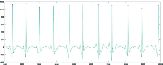

  

  R point location

• Heart Beats Segmentation

Find two adjacent R points, resampling the waveform between the R-R, then splicing the two adjacent waveforms to obtain a complete heart beat. Standardizing the number of sample points as 250, we randomly intercepted the two groups of heart beats, as shown in Fig. 2.

Fig. 2.

Heart beat segmentation

3.2 Feature Extraction

Based on whitening and PCA, the initial heart beats correlation is removed, and the dimensionality of heart beats is reduced from 250 to 30. Assuming heart beats $X \in R^{{{\text{m}} \times {\text{n}}}}$, where m is the number of beats, n is the dimensionality of the heart beats, all heart beats are aligned with the start and end points. Each heart beat has 250 points and the length is the same [11].

• Whitening Step

Whitening eliminates the correlation between ECG data and allows further analysis to be focused on higher order statistics, which can lead to a significant increase in subsequent processing speed. The specific steps are as follows.

• 1. Calculate the covariance matrix:

  $$ \Sigma = \frac{1}{\text{m}}XX^{T} $$

  (1)

• 2. Singular value decomposition of the covariance matrix:

  $$ [U,S,V] = svd(\Sigma ) $$

  (2)

  where U is the eigenvector matrix and S is the eigenvalue matrix.

• 3. Obtain the whitening beat data:

  $$ X_{\text{white}} = S^{{ - \frac{1}{2}}} U^{T} X $$

  (3)

  where $S^{{ - \frac{1}{2}}}$ is equivalent to the data on each spindle to do a scaling. Scaling factor is divided by the corresponding square root of the eigenvalue; $U^{T} X$ is the original data in the principal component axis projection.

• 4. Substitute the result of Step 3 into covariance matrix:

  $$ \sum {_{\text{white}} = \frac{1}{\text{m}}} X_{\text{white}} X_{\text{white}}^{T} = I $$

  (4)

The obtained covariance matrix is a unit matrix, each dimension becomes uncorrelated, and the variance of each dimension is 1. In practice, however, the eigenvalue of the heart beats may be close to zero, and the scaling step will result in dividing by a value close to zero. This may cause data overflow, so we introduce a regularization term that adds a small constant ɛ to the denominator of the eigenvalue matrix S to avoid affecting the feature. When X is normalized, $\varepsilon = 10^{ - 5}$.

• Dimensionality Reduction Step

PCA dimensionality reduction aims to greatly reduce the dimensionality of heart beat data and to express complete information with minimal feature quantity. The specific steps are as follows.

• 1. The heart beat data is organized in the form of m * n matrices to form a data set ${X_{{\rm{ij}}}} = \left[ {\matrix{{{{\rm{x}}_{{\rm{11}}}},{{\rm{x}}_{{\rm{12}}}}, \ldots ,{{\rm{x}}_{{\rm{1n}}}}}\\ {{{\rm{x}}_{21}}{\rm{,}}{{\rm{x}}_{22}}, \ldots ,{{\rm{x}}_{2{\rm{n}}}}}\\ \ldots \\ {{{\rm{x}}_{{\rm{m}}1}}{\rm{,}}{{\rm{x}}_{{\rm{m}}2}}, \ldots ,{{\rm{x}}_{{\rm{mn}}}}} } } \right]$, the set is normalized:

  $$ Z_{\text{ij}} = \frac{{X_{\text{ij}} - \overline{X}_{\text{j}} }}{{S_{\text{j}} }}\;\begin{array}{*{20}l} {{\text{i}} = 1,2, \ldots ,n} \hfill \\ {j = 1,2, \ldots ,m} \hfill \\ \end{array} $$

  (5)

  where $\overline{{X_{\text{j}} }} = \frac{{\sum\limits_{i = 1}^{n} {X_{ij} } }}{n}$ is the mean and $S_{\text{j}} = \sqrt {\frac{{\sum\limits_{i = 1}^{n} {(X_{ij} - \overline{{X_{j} }} )^{2} } }}{{{\text{n}} - 1}}}$ is the standard deviation.

• 2. Calculate the eigenvalues of the correlation coefficient matrix and obtain m eigenvalues:

  $$ R = \frac{{Z^{T} Z}}{{{\text{n}} - 1}} $$

  (6)

• 3. Determine the p value:

  $$ \frac{{\sum\limits_{{{\text{j}} = 1}}^{p} {\lambda_{j} } }}{{\sum\limits_{j = 1}^{m} {\lambda_{j} } }} \ge {\text{a}} $$

  (7)

  where a is the contribution rate of the components, usually more than 90%. For each eigenvalue $\lambda_{\text{j}}$, solving $R{\text{d}} = \lambda_{\text{j}} {\text{d}}$ obtains unit eigenvector ${\text{d}}_{\text{j}}^{\text{o}}$.

• 4. Conversion to the main components:

  $$ Y_{\text{j}} = Z_{\text{i}}^{T} {\text{d}}_{\text{j}}^{\text{o}} $$

  (8)

In general, only the first few variables are the main components, we should calculate whether the contribution rate meets the requirements.

3.3 Classification

According to the principle of RPROP algorithm, the learning rate is changed by the gradient direction according to the local adaptive strategy, which makes the convergence stable, fast and not easy to fall into the local minimum. The specific steps are as follows.

①:

Similar to the traditional BP algorithm, the number of neurons in each layer was set on the basis of heart beat samples, PCA feature dimensionality and the number of classes. Let i, j, k be the number of neurons in the input layer, hidden layer and output layer, respectively.

②:

Initialize the variable speed $\Delta_{\text{ji}}^{(0)}$, variable speed factor $\upsilon$, lower threshold $\Delta_{ \hbox{min} }$ and upper threshold $\Delta_{ \hbox{max} }$.

③:

Calculate the error between actual output and expected output: $E(t) = \frac{1}{2}\sum\limits_{{{\text{k}} = 1}}^{\text{n}} {(o_{1k} - o_{2k} )^{2} }$, where $o_{1k}$ is the actual output, $o_{2k}$ is the desired output.

④:

Judge the relationship between the value of $\frac{{\partial E^{{ ( {\text{k}} - 1 )}} }}{{\partial W_{ji} }} * \frac{{\partial E^{(k)} }}{{\partial W_{ji} }}$ and 0. If the value is equal to 0, go to step ⑤; if greater than 0, go to step ⑥; if less than 0, go to step ⑦.

⑤:

Weight update item $\Delta_{\text{ji}}^{{ ( {\text{k)}}}} = \Delta_{\text{ji}}^{{ ( {\text{k}} - 1 )}}$ needs no change.

⑥:

Weight update item $\Delta_{\text{ji}}^{{ ( {\text{k)}}}} = {\text{min(}}\Delta_{\text{ji}}^{{ ( {\text{k}} - 1 )}} \cdot \upsilon^{ + } ,\Delta_{ \hbox{max} } )$, for increasing the update value. We take $\upsilon^{ + } = 1.2$ generally.

⑦:

Weight update item $\Delta_{\text{ji}}^{{ ( {\text{k)}}}} = {\text{max(}}\Delta_{\text{ji}}^{{ ( {\text{k}} - 1 )}} \cdot \upsilon^{ - } ,\Delta_{ \hbox{min} } )$, for reducing the update value. We take $\upsilon^{ - } = 0.5$ generally.

⑧:

According to the above steps, adjust the weight $W_{\text{ji}}^{{ ( {\text{k)}}}} = W_{\text{ji}}^{{ ( {\text{k}} - 1 )}} - {\text{sgn}}(\frac{{\partial E^{(k)} }}{{\partial W_{ji} }})\Delta_{ji}^{(k)}$.

⑨:

Take the minimum gradient of 1.0-e7, limit the iteration times to 500, and judge if the error E reaches the setting value, and if not, back to step ③; if so, end the training process, save the training model, and record the training time.

By this method, we optimize the classifier of ECG identification and improve the classification stability.

3.4 Identification

The principle of hierarchical voting is applied in identification, which uses the resulting confusion matrix obtained by the above classification algorithm as the voting data source. The registration database and the identification database are then compared one by one, and the majority of voting is used as the final recognition result. Figure 3 is the complete flow chart of ECG identification.

Fig. 3.

ECG identification flow chart

4 Experiments and Results

4.1 Database

This data is obtained from the ECG-ID database in PhysioNet (www.physionet.org), which contains the ECG signals of 88 persons, 20 s per person on average, with a digital frequency of 500 Hz and a resolution of 12 bits. Everyone has no less than two sets of signals collected at different times, all signals can be obtained freely from the website. The experiment goal is to identify the 88 persons. The identification process is shown in Fig. 4.

Fig. 4.

Recognition process

4.2 Preprocessing and NN Model Setting

Select two different times from the database of the heart beats, about 20 s each time, from a total of 88 people. After denoising, locating R points and obtaining individual heart beats, we resample 250 points from the beats and align the start and end points. We then perform PCA whitening, extract PCA feature, and reduce the dimensionality to 30. We take 2055 beats at time A as the training set and 2103 at time B as the testing set for neural networks training and testing respectively. The number of neurons in the output layer is the number of people. We set the number of neurons in the hidden layer based on the classical formula ${\text{a}} = \sqrt {{\text{b}} + {\text{c}}} + {\text{r}}$ (b is the number of input layers, c is the number of output layers, r = 1–10), and this forms a single hidden layer neural network classification model of 30-20-88 neurons. For RPROP algorithm, we set the iteration times as 500, the error standard as 0.0005, the minimum gradient as 1e-7, the initial shift value as 0.07, and the threshold values as 50 and 0.001 respectively.

4.3 Experiment

A complete ECG system consists of three parts: signal preprocessing, feature extraction, classification. We have denoised the ECG signal during signal preprocessing as described above, and now the focus of the experiment will be on feature extraction and classification algorithm.

• Comparison of initial feature extraction:

This paper adopts the method of locating single R point to extract complete heart beats as the initial features. To evaluate its effectiveness, we compare it with the following two methods.

Wavelet coefficients: Discrete wavelet transform coefficients are extracted for identification. Because the 2-layer wavelet (DB2) has good smooth characteristic, it is suitable to detect the change of the ECG signal. Also, the different frequency of the heart beats is mainly concentrated in the third and fourth scales. Therefore, we take the third and fourth scale coefficients and the detail coefficients as feature.

QRS wave: The left third pole of R point is Q point and the right third pole is S point. We locate Q and S points this way, and take the QRS wave and the points’ intervals, amplitudes as feature.

• Comparison of PCA whitening and non-PCA whitening:

Because of the influence of PCA whitening on the efficiency of classification, we separate the initial features into PCA whitening and non-PCA whitening. Figure 5 shows the initial features of three persons (represented by A, B and C) which are selected from the database randomly. Figure 6 shows their PCA whitening features. The solid line is the features of tester A at three different times, and the dotted lines are the features of tester B and C. From Fig. 6, we can see that the features of tester A at different times almost coincide, but different from others. Therefore, the PCA whitening features of ECG signals have obvious advantages over ECG identification.

• Comparison of classifiers:

We use PCA to reduce the feature dimensionality from 250 to 30, yet the 30 principal components can still provide 98.75% contribution. As shown in Fig. 7, the first 10 principal components can actually reach a comprehensive contribution of close to 90%. Under the same standard, we take the heart beats of the same person in different times as training set and test set. The accuracy and efficiency of KNN, SVM, traditional BP and RPROP algorithm are compared respectively. Figure 8 shows the error convergence of RPROP algorithm and L-M algorithm under the same set. As one can see, compared with L-M algorithm (based on amount of gradient), the RPROP (based on the direction of gradient) has a faster and smoother convergence.

Fig. 5.

Initial features of heart beat

Fig. 6.

PCA whitening feature

Fig. 7.

Principal component contribution rate

Fig. 8.

Error convergence curve of RPROP and L-M

4.4 Results and Analysis

The classification accuracy of three initial features with LIBSVM [12] is shown in Table 1.

Table 1. Accuracy of different initial features (%)

Table 1 is shows that the effective information of our complete beat feature extraction method is higher than QRS wave and wavelet coefficient. Given that location only involves R points, our method of extracting the initial features is simple and more efficient.

In order to save test time in experiment, we compared the time consumed by using PCA whitening data and the results are shown in Table 2. We compared the feature of PCA with that of non-PCA in each classifier to test the effect of PCA whitening. The results of classification are shown in Fig. 9.

Table 2. The training time of different classifiers

Fig. 9.

Classification accuracy

Table 2 shows that the our RPROP based approach only takes about 10 s, which is much more efficient than the other three classifiers. It can be seen from Fig. 8 that the features processed by PCA whitening yield slightly higher accuracy than the unprocessed feature. Compared with the other three classification methods, the recognition accuracy of our RPROP approach is obviously higher than traditional BP algorithm. In terms of PCA whitening, the accuracy of the RPROP method is 96.6%, which is 2.4% higher than SVM. The time efficiency is 14 s faster than KNN.

5 Conclusion

In order to improve the accuracy and efficiency of ECG identification, we conducted an experimental study in feature extraction, classification and recognition. By comparing a series of methods, the information integrity of the proposed complete heart beat features is seen to be superior to the features through other methods such as wavelet coefficient, QRS wave, and the classification accuracy also higher than the other features under LIBSVM. The complexity and redundancy of proposed features are significantly reduced by PCA whitening. The paper selected the optimal features as input to the neural network that is further optimized by RPROP algorithm for classification. The accuracy of the PCA-RPROP algorithm is higher than KNN, SVM and BP, reaching 96.6%. This demonstrates the validity of PCA-RPROP algorithm for ECG identification. Because of its obvious time efficiency in recognition, it can be used as a core algorithm for engineering a complete ID system.

ECG signals are frequently applied in monitoring patient’s heart rate status and adjuvant therapy. Likewise, simple and effective ECG identification can be widely used in identity recognition in a variety of applications, such as drug use management, privacy protection, medical treatment recording and other remote medical identification without additional data.

References

Biel, L., Pettersson, O., Philipson, L., et al.: ECG analysis: a new approach in human identification. IEEE Trans. Instrum. Meas. 50, 808–812 (2001)
Palaniappan, R., Krishnan, S.M.: Identifying individuals using ECG beats. In: International Conference on Signal Processing and Communications, Bangalore, India, pp. 569–572 (2005)
Israel, S.A., Irvine, J.M., Cheng, A., et al.: ECG to identify individuals. Pattern Recogn. 38, 133–142 (2005)
Plataniotis, K.N., Hatzinakos, D., Lee, J.K.M.: ECG biometric recognition without fiducial detection. In: Biometric Consortium Conference, 2006 Biometrics Symposium: Special Session on Research, Baltimore, MD, pp. 1–6 (2006)
Jégou, H., Chum, O.: Negative evidences and co-occurrences in image retrieval: the benefit of PCA and whitening. In: Fitzgibbon, A., Lazebnik, S., Perona, P., Sato, Y., Schmid, C. (eds.) ECCV 2012. LNCS, pp. 774–787. Springer, Heidelberg (2012). doi:10.1007/978-3-642-33709-3_55
Moré, J.J.: The Levenberg-Marquardt algorithm: implementation and theory. In: Watson, G.A. (ed.) Numerical Analysis. LNM, vol. 630, pp. 105–116. Springer, Heidelberg (1978). doi:10.1007/BFb0067700
Riedmiller, M., Braun, H.: A direct adaptive method for faster backpropagation learning: the RPROP algorithm. In: IEEE International Conference on Neural Networks, San Francisco, CA, vol. 1, pp. 586–591 (1993)
Saxena, S.C., Kumar, V., Hamde, S.T.: Feature extraction from ECG signals using wavelet transforms for disease diagnostics. Int. J. Syst. Sci. 33, 1073–1085 (2002)
Han, X.U., Wang, D.D., Jiang, T.B.: Research on the ECG signal denoising algorithm based on wavelet transform and the median filter. Autom. Instrum. (2012)
Sadhukhan, D., Mitra, M.: R-peak detection algorithm for ECG using double difference and RR interval processing. Procedia Technol. 4, 873–877 (2012)
Marrtis, R.J., Acharya, U.R., Min, L.C.: ECG beat classification using PCA, LDA, ICA and discrete wavelet transform. Biomed. Signal Process. Control 8, 437–448 (2013)
Chang, C.C., Lin, C.J.: LIBSVM: a library for support vector machines. ACM Trans. Intell. Syst. Technol. 2, 27 (2011)
Acknowledgment
We thank all the volunteers and colleagues provided helpful comments on previous versions of the manuscript. This work was supported by the Science and Technology Development projects funded by Jilin Government (20150204039GX, 20170414017GH), Science and Technology Development Special Funded by Guangdong Government (2016A030313658), and Key Scientific and Technological Special Fund Project supported by Changchun Government under Grant No. 14KG064. This work was also supported by Premier-Discipline Enhancement Scheme Supported by Zhuhai Government and Premier Key-Discipline Enhancement Scheme Supported by Guangdong Government Funds.
Author information
Authors and Affiliations
Corresponding author
Editor information
Editors and Affiliations
Rights and permissions
Copyright information
© 2017 Springer International Publishing AG
About this paper
Cite this paper
Yu, J., Si, Y., Liu, X., Wen, D., Luo, T., Lang, L. (2017). ECG Identification Based on PCA-RPROP. In: Duffy, V. (eds) Digital Human Modeling. Applications in Health, Safety, Ergonomics, and Risk Management: Health and Safety. DHM 2017. Lecture Notes in Computer Science(), vol 10287. Springer, Cham. https://doi.org/10.1007/978-3-319-58466-9_37
Download citation
DOI: https://doi.org/10.1007/978-3-319-58466-9_37
Published:
Publisher Name: Springer, Cham
Print ISBN: 978-3-319-58465-2
Online ISBN: 978-3-319-58466-9
eBook Packages: Computer ScienceComputer Science (R0)