Vectors

Abstract

After reading this chapter you know:

• what vectors are and how they can be used,

• how to algebraically perform and geometrically represent addition and subtraction of vectors,

• how to algebraically perform and intuitively understand common forms of vector multiplication and

• how vector relationships can be expressed and what their use is.

Appendices

Symbols Used in This Chapter (in Order of Their Appearance)

$\overrightarrow{\cdot}$	Vector
$\overrightarrow{i}$, $\overrightarrow{j}$, $\overrightarrow{k}$	Vectors of length 1 along the principal x-, y-, and z-axes
$\left|\overrightarrow{\cdot}\right|$	Vector norm
ϕ	Here: angle between two vectors
⋅	Inner product
cos	Cosine
adj	Edge in a right-angled triangle adjacent to the acute angle
$\overrightarrow{n}$	Normal vector
×	Here: cross product
sin	Sine
opp	Edge in a right-angled triangle opposite to the acute angle cross product
cov	Covariance
σ	Standard deviation
${\overrightarrow{\cdot}}_{\perp }$	Orthogonalized vector

Overview of Equations, Rules and Theorems for Easy Reference

Addition and subtraction of vectors

$$ \overrightarrow{a}+\overrightarrow{b}+\overrightarrow{c}=\left(\begin{array}{c}\hfill {a}_1\hfill \\ {}\hfill \vdots \hfill \\ {}\hfill {a}_n\hfill \end{array}\right)+\left(\begin{array}{c}\hfill {b}_1\hfill \\ {}\hfill \vdots \hfill \\ {}\hfill {b}_n\hfill \end{array}\right)+\left(\begin{array}{c}\hfill {c}_1\hfill \\ {}\hfill \vdots \hfill \\ {}\hfill {c}_n\hfill \end{array}\right)=\left(\begin{array}{c}\hfill {a}_1+{b}_1+{c}_1\hfill \\ {}\hfill \vdots \hfill \\ {}\hfill {a}_n+{b}_n+{c}_n\hfill \end{array}\right) $$

Magnitude (length, module, absolute value, norm) of a vector

$$ \left|\overrightarrow{a}\right|=\left|\left(\begin{array}{c}\hfill {a}_1\hfill \\ {}\hfill \vdots \hfill \\ {}\hfill {a}_n\hfill \end{array}\right)\right|=\sqrt{a_1^2+\cdots +{a}_n^2} $$

Inner vector product

$$ \overrightarrow{a}\cdot \overrightarrow{b}=\left(\begin{array}{c}\hfill {a}_1\hfill \\ {}\hfill \vdots \hfill \\ {}\hfill {a}_n\hfill \end{array}\right)\cdot \left(\begin{array}{c}\hfill {b}_1\hfill \\ {}\hfill \vdots \hfill \\ {}\hfill {b}_n\hfill \end{array}\right)={a}_1{b}_1+\cdots {a}_n{b}_n\kern0.62em \mathrm{or} $$

$$ \overrightarrow{a}\cdot \overrightarrow{b}=\left|\overrightarrow{a}\right|\left|\overrightarrow{b}\right|\cos \varphi, $$

where 0 < φ < π is the angle between $\overrightarrow{a}$ and $\overrightarrow{b}$ when they originate at the same position.

Definition of a plane through the origin

$$ \overrightarrow{n}\cdot \overrightarrow{x}=0, $$

where $\overrightarrow{n}$ is a normal vector, perpendicular to the plane and $\overrightarrow{x}$ is any vector such that $\overrightarrow{n}\cdot \overrightarrow{x}=0$

Cross vector product

$$ \overrightarrow{a}\times \overrightarrow{b}=\left(\begin{array}{c}\hfill {a}_1\hfill \\ {}\hfill {a}_2\hfill \\ {}\hfill {a}_3\hfill \end{array}\right)\times \left(\begin{array}{c}\hfill {b}_1\hfill \\ {}\hfill {b}_2\hfill \\ {}\hfill {b}_3\hfill \end{array}\right)=\left(\begin{array}{c}\hfill {a}_2{b}_3-{a}_3{b}_2\hfill \\ {}\hfill {a}_3{b}_1-{a}_1{b}_3\hfill \\ {}\hfill {a}_1{b}_2-{a}_2{b}_1\hfill \end{array}\right)\kern0.5em \mathrm{or} $$

$$ \overrightarrow{a}\times \overrightarrow{b}=\left|\overrightarrow{a}\right|\left|\overrightarrow{b}\right|\sin \varphi\;\overrightarrow{n} $$

where 0 < φ < π is the angle between $\overrightarrow{a}$ and $\overrightarrow{b}$ when they originate at the same position and $\overrightarrow{n}$ is a unit vector.

Correlation coefficient

The sample correlation between two random demeaned variables X and Y as defined by Pearson’s correlation coefficient is given by:

$$ r\left(X,Y\right)=\frac{\frac{1}{n-1}\sum \limits_{i=1}^n{x}_i{y}_i}{\sqrt{\frac{1}{n-1}\sum \limits_{i=1}^n{x}_i^2}\sqrt{\frac{1}{n-1}\sum \limits_{i=1}^n{y}_i^2}}=\frac{\sum \limits_{i=1}^n{x}_i{y}_i}{\sqrt{\sum \limits_{i=1}^n{x}_i^2}\sqrt{\sum \limits_{i=1}^n{y}_i^2}}=\frac{\overrightarrow{x}\cdot \overrightarrow{y}}{\left|\overrightarrow{x}\right|\left|\overrightarrow{y}\right|}=\cos \varphi $$

where $\overrightarrow{x}$ and $\overrightarrow{y}$ are two vectors representing the pairs of variables and 0 < φ < π is the angle between these vectors when they originate at the same position.

Projection

The projection of $\overrightarrow{a}$ on $\overrightarrow{b}$ is given by:

$$ \frac{\overrightarrow{a}\cdot \overrightarrow{b}}{{\left|\overrightarrow{b}\right|}^2}\overrightarrow{b} $$

(Gram-Schmidt) orthogonalization

The orthogonalization of two vectors ${\overrightarrow{a}}_1$ and ${\overrightarrow{a}}_2$ or the Gram-Schmidt orthogonalization of three vectors ${\overrightarrow{a}}_1$, ${\overrightarrow{a}}_2$ and ${\overrightarrow{a}}_3$ is given by:

$$ {\displaystyle \begin{array}{l}{\overrightarrow{a}}_{1,\perp }={\overrightarrow{a}}_1\\ {}{\overrightarrow{a}}_{2,\perp }={\overrightarrow{a}}_2-\frac{{\overrightarrow{a}}_2\cdot {\overrightarrow{a}}_{1,\perp }}{{\left|{\overrightarrow{a}}_{1,\perp}\right|}^2}{\overrightarrow{a}}_{1,\perp}\\ {}{\overrightarrow{a}}_{3,\perp }={\overrightarrow{a}}_3-\frac{{\overrightarrow{a}}_3\cdot {\overrightarrow{a}}_{1,\perp }}{{\left|{\overrightarrow{a}}_{1,\perp}\right|}^2}{\overrightarrow{a}}_{1,\perp }-\frac{{\overrightarrow{a}}_3\cdot {\overrightarrow{a}}_{2,\perp }}{{\left|{\overrightarrow{a}}_{2,\perp}\right|}^2}{\overrightarrow{a}}_{2,\perp }.\end{array}} $$

Answers to Exercises

• 4.1. The sum and difference of the two vectors are:

  • (a) $\left(\begin{array}{c}\hfill 9\hfill \\ {}\hfill 7\hfill \end{array}\right)$ and $\left(\begin{array}{c}\hfill 5\hfill \\ {}\hfill -1\hfill \end{array}\right)$

  • (b) $\left(\begin{array}{c}\hfill 1\hfill \\ {}\hfill 3\hfill \end{array}\right)$ and $\left(\begin{array}{c}\hfill -5\hfill \\ {}\hfill 31\hfill \end{array}\right)$

  • (c) $\left(\begin{array}{c}\hfill 5\hfill \\ {}\hfill -21\hfill \\ {}\hfill 10\hfill \end{array}\right)$ and $\left(\begin{array}{c}\hfill -3\hfill \\ {}\hfill 25\hfill \\ {}\hfill -4\hfill \end{array}\right)$

  • (d) $\left(\begin{array}{c}\hfill 3.6\hfill \\ {}\hfill 4.8\hfill \\ {}\hfill 9\hfill \\ {}\hfill 7.8\hfill \end{array}\right)$ and $\left(\begin{array}{c}\hfill 1.2\hfill \\ {}\hfill -2.4\hfill \\ {}\hfill -1.8\hfill \\ {}\hfill 3\hfill \end{array}\right)$

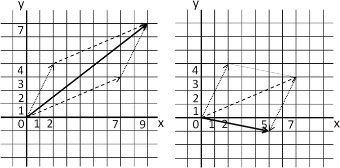
• 4.2. The vector $\left(\begin{array}{c}\hfill 7\hfill \\ {}\hfill 3\hfill \end{array}\right)$ is indicated with a dashed arrow and the vector $\left(\begin{array}{c}\hfill 2\hfill \\ {}\hfill 4\hfill \end{array}\right)$ is indicated with a dotted arrow, both starting at the origin. The geometrical sum of the two vectors is indicated in the left figure and the geometrical difference of the two vectors is indicated in the right figure, both by a drawn arrow. Some additional lines and copies of the (negative of the) arrows are indicated to visualize the supporting parallelogram.

  

• 4.3.

  • (a) $\left(\begin{array}{c}\hfill -2\hfill \\ {}\hfill 3\hfill \\ {}\hfill -21\hfill \end{array}\right)$

  • (b) $\left(\begin{array}{c}\hfill 3.5\hfill \\ {}\hfill 0\hfill \\ {}\hfill 2.9\hfill \end{array}\right)$

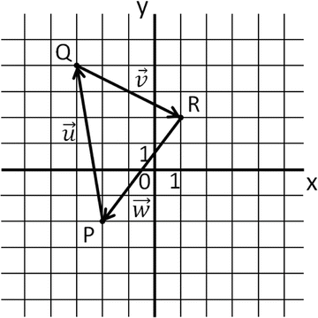
• 4.4. P = (−2,−2), Q = (−3,4) and R = (1,2).

• (a) Below, the points P, Q and R and their connecting vectors have been drawn.

  

• (b) $\overrightarrow{u}=\left(\begin{array}{c}\hfill -1\hfill \\ {}\hfill 6\hfill \end{array}\right)$, $\overrightarrow{v}=\left(\begin{array}{c}\hfill 4\hfill \\ {}\hfill -2\hfill \end{array}\right)$ and $\overrightarrow{w}=\left(\begin{array}{c}\hfill -3\hfill \\ {}\hfill -4\hfill \end{array}\right)$

• (c) The null vector (after connecting—i.e. adding—all vectors, we end up in the same location).

• 4.5.

  • (a) One minute is 1/60th hour, thus the location of the airplane after 1  min is the velocity vector divided by 60: (3.33, 3, 1.66).

  • (b) 100  m is 0.1  km. The airplane climbs 100  km in 1  h, thus 0.1  km in 1/1000 h = 3.6 s.

  • (c) It takes 3.6 s to climb 100 m, thus 3.6 × 10 × 9 = 324 s to climb to 9 km.

• 4.6. The inner product of each of these pairs of vectors is

  • (a) 0

  • (b) 0

  • (c) 15

  • (d) 4

  • (e) 1

• 4.7. The inner product of each of these pairs of vectors is

  • (a) 35

  • (b) 0

  • (c) 7.2

  • (d) −1

• 4.8. Use that $\overrightarrow{a}\cdot \overrightarrow{b}=\left|\overrightarrow{a}\right|\left|\overrightarrow{b}\right|\cos \varphi$.

  • (a) $\cos \varphi =1/\sqrt{17}$, thus φ ≈ 76^°

  • (b) cos φ =  − 2/2 =  − 1, thus φ = 180^°

  • (c) $\cos \varphi =15/\sqrt{5}\cdot \sqrt{45}=15/\sqrt{225}=15/15=1$, thus φ = 0^°

  • (d) $\cos \varphi =7/\sqrt{10}\cdot \sqrt{17}$, thus φ ≈ 58^°

  • (e) $\cos \varphi =1/\sqrt{5}\cdot \sqrt{10}$, thus φ ≈ 82^°

• 4.9.

  • (a) x − 2y + 3z = 0

  • (b) In general, a plane with normal vector $\left(\begin{array}{c}\hfill -1.5\hfill \\ {}\hfill 0.5\hfill \\ {}\hfill 2\hfill \end{array}\right)$ is given by −1.5x + 0.5y + 2z = C. To find C, we substitute the point $\left(\begin{array}{c}\hfill 2\hfill \\ {}\hfill 4\hfill \\ {}\hfill -3\hfill \end{array}\right)$ that is in the plane: −1.5⋅2 + 0.5⋅4–3⋅2 = −3 + 2 – 6 = −7 and thus this plane is given by −1.5x + 0.5y + 2z = −7.

• 4.10.

  • (a) any combination of x, y and z that satisfies x − 2y + 3z = 0 is a point in the plane, e.g. (−1, 1, 1) or (2, 2, 2/3).

  • (b) similar to 4.10(a), (1, 1, −3) is a point in this plane, but also (0, 0, −3.5).

• 4.11. The work performed by the object is determined by the formula work = F ⋅ d ⋅ cos(α), where F is the force (in N), d the displacement (in m) and α the angle between the displacement and the force.

  • (a) work = 10⋅3⋅4/5 = 90/5 = 18

  • (b) work = 15⋅4⋅4/5 = 180/5 = 36

• 4.12.

  • (a) $\left(\begin{array}{c}\hfill 1\hfill \\ {}\hfill 1\hfill \\ {}\hfill 2\hfill \end{array}\right)\times \left(\begin{array}{c}\hfill 2\hfill \\ {}\hfill 3\hfill \\ {}\hfill 4\hfill \end{array}\right)=\left(\begin{array}{c}\hfill 4-6\hfill \\ {}\hfill -\left(4-4\right)\hfill \\ {}\hfill 3-2\hfill \end{array}\right)=\left(\begin{array}{c}\hfill -2\hfill \\ {}\hfill 0\hfill \\ {}\hfill 1\hfill \end{array}\right)$

  • (b) $\left(\begin{array}{c}\hfill 1\hfill \\ {}\hfill 0\hfill \\ {}\hfill -2\hfill \end{array}\right)\times \left(\begin{array}{c}\hfill -5\hfill \\ {}\hfill 2\hfill \\ {}\hfill 7\hfill \end{array}\right)=\left(\begin{array}{c}\hfill 0+4\hfill \\ {}\hfill -\left(7-10\right)\hfill \\ {}\hfill 2-0\hfill \end{array}\right)=\left(\begin{array}{c}\hfill 4\hfill \\ {}\hfill 3\hfill \\ {}\hfill 2\hfill \end{array}\right)$

  • (c) $\left(\begin{array}{c}\hfill -1\hfill \\ {}\hfill -1\hfill \\ {}\hfill -1\hfill \end{array}\right)\times \left(\begin{array}{c}\hfill 0.2\hfill \\ {}\hfill 0.3\hfill \\ {}\hfill 0.4\hfill \end{array}\right)=\left(\begin{array}{c}\hfill -0.4+0.3\hfill \\ {}\hfill -\left(-0.4+0.2\right)\hfill \\ {}\hfill -0.3+0.2\hfill \end{array}\right)=\left(\begin{array}{c}\hfill -0.1\hfill \\ {}\hfill 0.2\hfill \\ {}\hfill -0.1\hfill \end{array}\right)$

• 4.13. Remember that a plane is determined by its normal vector and that a normal vector can be determined by the cross product of two points (vectors) in the plane.

  • (a) the normal vector for this plane is given by

$\left(\begin{array}{c}\hfill 1\hfill \\ {}\hfill 1\hfill \\ {}\hfill 1\hfill \end{array}\right)\times \left(\begin{array}{c}\hfill 2\hfill \\ {}\hfill 3\hfill \\ {}\hfill 4\hfill \end{array}\right)=\left(\begin{array}{c}\hfill 4-3\hfill \\ {}\hfill -\left(4-2\right)\hfill \\ {}\hfill 3-2\hfill \end{array}\right)=\left(\begin{array}{c}\hfill 1\hfill \\ {}\hfill -2\hfill \\ {}\hfill 1\hfill \end{array}\right)$,

thus the plane (through the origin) is x − 2y + z = 0.

• (b) the normal vector for this plane is given by

$\left(\begin{array}{c}\hfill 2\hfill \\ {}\hfill 1\hfill \\ {}\hfill -1\hfill \end{array}\right)\times \left(\begin{array}{c}\hfill 2\hfill \\ {}\hfill 3\hfill \\ {}\hfill 4\hfill \end{array}\right)=\left(\begin{array}{c}\hfill 4+3\hfill \\ {}\hfill -\left(8+2\right)\hfill \\ {}\hfill 6-2\hfill \end{array}\right)=\left(\begin{array}{c}\hfill 7\hfill \\ {}\hfill -10\hfill \\ {}\hfill 4\hfill \end{array}\right)$,

Thus the plane (through the point (1, 1, 1)) is 7x − 10y + 4z = 1.

• 4.14. Tip: remember that two vectors $\overrightarrow{a}$ and $\overrightarrow{b}$ are dependent if there is a scalar s such that $s\overrightarrow{a}=\overrightarrow{b}$, correlated if $\left(\overrightarrow{a}-\overline{a}\right)\cdot \left(\overrightarrow{b}-\overline{b}\right)=0$ (where $\overline{\cdot}$ denotes the mean over all vector elements) and orthogonal if $\overrightarrow{a}\cdot \overrightarrow{b}=0$

  • (a) independent, correlated and not orthogonal

  • (b) independent, uncorrelated and not orthogonal

  • (c) independent, correlated and orthogonal

  • (d) independent, uncorrelated and orthogonal

  • (e) dependent, correlated and not orthogonal

Glossary

Algebraically

Using an expression in which only mathematical symbols and arithmetic operations are used.

Associativity

Result is the same independent of how numbers are grouped (true for addition and multiplication of more than two numbers; see Box 4.1 ).

Commutativity

Result is the same independent of the order of the numbers (true for addition and multiplication; see Box 4.1 ).

Coordinates

Pairs (2D space) or triplets (2D space) of ordered numbers that determine a point’s position in space.

Covariance

A measure of joint variability of two random variables; if the two variables jointly increase and jointly decrease the covariance is positive, if one variable increases when the other decreases and vice versa, the covariance is negative.

Demeaned

A set of variables from which the mean has been subtracted, i.e. with zero mean (also known as centered).

Determinant

Property of a square matrix, which can be thought of as a scaling factor of the transformation the matrix represents (see also Chap. 5 ).

Distributivity

Result is the same for multiplication of a number by a group of numbers added together, and each multiplication done separately after which all multiplications are added (in this case the algebraic expression is really much easier to understand than the words; see Box 4.1 ).

Electromyography

Measurement of electrical muscle activity by (surface or needle) electrodes.

Element

As in ‘vector element’: one of the entries in a vector.

Geometrically

Using geometry and its methods and principles.

Geometry

The branch of mathematics dealing with shapes, sizes and other spatial features.

iff

‘If and only if’: math lingo for a relation that holds in two directions, e.g. a iff b means ‘if a then b and if b then a’.

Linear combination

The result of multiplying a set of terms with constants and adding them.

Linear dependence

Two vectors having the same orientation, differing only in their length.

Matrix

A rectangular array of (usually) numbers.

Multicollinearity

Two or more of a set of vectors or regressors are highly correlated or one of the vectors or regressors in this set is (almost) a linear combination of the others.

Multiple linear regression

Predicting a dependent variable from a set of independent variables according to a linear model.

Norm

Length or size of a vector.

Normal vector

A vector that is perpendicular to a plane.

Null vector

The result of subtracting a vector from itself.

Orthogonal

Two vectors that are geometrically perpendicular or equally, have an inner product of zero.

Orthogonalize

To make (two vectors) orthogonal.

Parallelepiped

3D figure formed by six parallelograms (it relates to a parallelogram like a cube relates to a square).

Parallelogram

A quadrilateral with two pairs of parallel sides (note that a square is a parallelogram, but not every parallelogram is square).

Regressor

An independent variable that can explain a dependent variable in a regression model, represented by a vector in the regression model

Scalar

Here: a real number that can be used for scalar multiplication in which a vector multiplied by a scalar results in another vector.

Unit vector

A vector divided by its own length, resulting in a vector with length one.

Vector

Entity with a magnitude and direction, often (geometrically) indicated by an arrow.

Voxel

Here: a sample of brain activation as measured on a 3D rectangular grid.

Work

Product of the force exerted on an object and its displacement.