Trigonometry

Abstract

After reading this chapter you know:

• what the three main trigonometric ratios are and how they can be calculated,

• how to express angles in degrees and radians,

• how to sketch the three main trigonometric functions,

• how to sketch functions of the form A sin(Bx + C) + D and how to interpret A, B, C and D,

• what Fourier (or spectral or harmonic) analysis is and

• how Fourier analysis is used in real-life examples.

Appendices

Symbols Used in This Chapter (in Order of Their Appearance)

sin	Sine
cos	Cosine
tan	Tangent
$\underset{x\to 0}{\lim \limits }$	Limit for x approaching zero
α,θ,ϕ	Angles
r,R	Radius (of a circle)
rad	Radian
e	Exponential
i	Imaginary unit
∑	Sum
∫	Integral
f	Frequency
t	Time
ω	Angular frequency

Overview of Equations, Rules and Theorems for Easy Reference

Mnemonic for memorizing trigonometric ratios

sine = O/H

cosine = A/H

tangent = O/A = sine/cosine

where O = opposite, A = adjacent, H = hypothenuse

Angles and values to remember

x in rad	π/6	π/4	π/3	π/2	π
sin(x)	0.5	$\frac{1}{2}\sqrt{2}$	$\frac{1}{2}\sqrt{3}$	1	0

Euler’s formula

$$ {e}^{ix}=\cos (x)+i\sin (x) $$

Trigonometric relations

$$ {\mathrm{sin}}^2(x)+{\mathrm{cos}}^2(x)=1 $$

$$ {\displaystyle \begin{array}{l}\cos \left(x+y\right)=\cos (x)\cos (y)-\sin (x)\sin (y)\\ {}\sin \left(x+y\right)=\cos (x)\sin (y)+\sin (x)\cos (y)\end{array}} $$

$$ {\displaystyle \begin{array}{l}\cos \left(x-y\right)=\cos (x)\cos (y)+\sin (x)\sin (y)\\ {}\sin \left(x-y\right)=\sin (x)\cos (y)-\cos (x)\sin (y)\end{array}} $$

$$ {\displaystyle \begin{array}{l}\sin (2x)=2\sin (x)\cos (x)\\ {}\cos (2x)={\mathrm{cos}}^2(x)-{\mathrm{sin}}^2(x)\end{array}} $$

$$ \cos (2x)=1-2{\mathrm{sin}}^2(x) $$

Answers to Exercises

• 3.1. The ratios must be calculated for the angle θ, so the sine, e.g., is always the length of the edge opposite from θ divided by the length of the hypothenuse etcetera. Sometimes rotating the triangles in your mind to relate them to the triangles in Fig. 3.3 will help. Thus the answers are for the left triangle: sine = 4/5, cosine = 3/5, tangent = 4/3, middle triangle: sine = 4/7, cosine = √33/7, tangent = 4/√33, right triangle: sine = 3/5, cosine = 4/5, tangent = 3/4.

• 3.2 First the lengths of the edges of the two triangles that angles 1 to 4 belong to must be determined. For angle 1, the adjacent edge is 75 cm long; this is the opposite edge for angle 2. For angle 2, the adjacent edges is 45 cm long; this is the opposite edge for angle 1. Similarly, the adjacent edge for angle 3 (opposite edge angle 4) is 65 cm long and the adjacent edge for angle 4 (opposite edge angle 3) is 35 cm long. The angles can now be determined by using the trigonometric ratio for the tangent: tan = O/A. Thus, $\tan \angle 1=\frac{45}{75}$, $\tan \angle 2=\frac{75}{45}$, $\tan \angle 3=\frac{35}{65}$ and $\tan \angle 4=\frac{65}{35}$. A calculator can now be used to determine the angles using the inverse tangent (or atan) function.

• 3.3

  • (a) 30° = 30*2π/360 = π/6 rad

  • (b) 45° = 45*2π/360 = π/4 rad

  • (c) 60° = 60*2π/360 = π/3 rad

  • (d) 80° = 80*2π/360 = 4/9 π rad

  • (e) 90° = 80*2π/360 = π/2 rad

  • (f) 123° = 123*2π/360 = 123/180 π rad

  • (g) (g) 260° = 260*2π/360 = 13/9 π rad

  • (h) (h) -16° = −16*2π/360 = −4/45 π rad

  • (i) -738° = −738 + 2*360° = −18° = −18*2π/360 = −1/10 π rad

• 3.4.

  • (a) 2π/3 rad = 2π/3*360/2π° = 120°

  • (b) π/4 rad = π/4*360/2π° = 45°

  • (c) 9π/4 rad = 9π/4-2π rad = π/4*360/2π° = 45°

  • (d) 0.763π rad = 0.763 π *360/2π° = 137,34°

  • (e) π rad = π*360/2π° = 180°

  • (f) θπ rad = θπ*360/2π° = 180θ°

  • (g) θ rad = θ*360/2π° = 180θ/π°

• 3.5.

  • (a) false: cos 0° = cos (0 rad) = 1

  • (b) false: sin 30° = sin (π/6 rad) = 0.5

  • (c) false: sin 45° = sin (π/4 rad) = $\frac{1}{2}\sqrt{2}$

  • (d) true

  • (e) false: cos 60° = cos(π/3 rad) = 0.5

• 3.6. For the angle of 60° the length of the opposite edge and the hypothenuse are x and 13, respectively. These two values can thus be used to calculate the sine of this angle by their ratio. But the sine of this angle is also equal to sin(60°) = sin(π/3 rad) = $\frac{1}{2}\sqrt{3}$. Thus x/13 = $\frac{1}{2}\sqrt{3}$, or x = $\frac{13}{2}\sqrt{3}$.

• 3.7. See Fig. 3.8 for the graphs of sin(x), cos(x) and tan(x). The exact values for the angles 0, 30, 45, 60 and 90 degrees (that help you make these sketches) are:

  degrees	rad	sin	cos	tan
  0	0	0	1	0
  30	π/6	0.5	$\frac{1}{2}\sqrt{3}$	$\frac{1}{3}\sqrt{3}$
  45	π/4	$\frac{1}{2}\sqrt{2}$	$\frac{1}{2}\sqrt{2}$	1
  60	π/3	$\frac{1}{2}\sqrt{3}$	0.5	$\sqrt{3}$
  90	π/2	1	0	∞

• 3.8.

  • (a) cos(−2x) = cos(2x)

  • (b) tan(−π/4) = −tan(π/4)

  • (c) sin(−4π/3) = −sin(4π/3)

• 3.9. sin(x): black, sin(2x): green, sin(x) + 2: red, sin(x + 2): magenta and 2 sin(x): blue.

• 3.10.

  • (a) For sketching y = 4sin(x), first make a table, with easily obtained values (making use of Table 3.1 and the trigonometric symmetries), e.g.:

    x	y
    -π ≅ − 3.14	0
    -π/2	−4
    -π/3	-$2\sqrt{3}$ ≅ − 3.46
    0	0
    π/3	$2\sqrt{3}$ ≅ 3.46
    π/2	4
    π	0

    Then sketch an x- and a y-axis to scale that are long enough to accommodate for the maximum (4) and minimum (−4) of the function and for at least one period (2π ≅ 6.28) of the function. Note that you are free to choose the scale of the axes. Put in the points you calculated in the table and sketch a smooth line through the points. Such a sketch could look like:

    

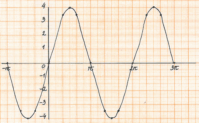
    Note that a sketch of a trigonometric function does not need to be limited to the positive x-axis: I here sketched it for both negative and positive values of x and also for more than one period.

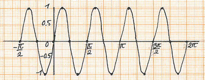
  • (b) For sketching y = sin(4x), first make a table, with easily obtained values (making use of Table 3.1 and the trigonometric symmetries), e.g.:

    x	y
    -π/4	0
    -π/8	−1
    -π/12	-$\frac{1}{2}\sqrt{3}$ ≅ − 0.87
    0	0
    π/12	$\frac{1}{2}\sqrt{3}$ ≅ 0.87
    π/8	1
    π/4	0

    Then sketch an x- and a y-axis to scale that are long enough to accommodate for the maximum (1) and minimum (−1) of the function and for at least one period (π/2 ≅ 1.57) of the function. Put in the points you calculated in the table and sketch a smooth line through the points. Such a sketch could look like:

    

• 3.11.

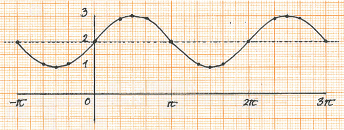
  • (a) Following a similar procedure as in Exercise 3.10 a sketch of y = 2 + sin(x) could look like:

    

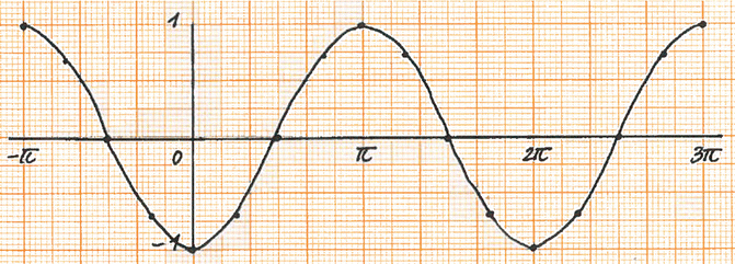
  • (b) Similarly, a sketch of y = − cos(x) could look like:

    

• 3.12.

  • (a) y =  − 3 sin(x) − 5 is obtained from the standard sine function by multiplying it by −3 and shifting it down by 5.

  • (b) y = 2 sin(3x) is obtained by multiplying it by 2 and changing the period to 2π/3 (if this last part is hard to grasp: the period is that number that you fill in for x, making the total between the brackets equal to 2π).

  • (c) y = 2 sin(x + π) + 2 is obtained by multiplying it by 2, shifting it up by 2 and shifting it to the left by π (again, it is to the left and not to the right because when I fill in -π, the value between brackets becomes 0).

  • (d) $y=3\sin \left(2x-\frac{\pi }{2}\right)-1$ is obtained by multiplying it by 3, shifting it down by 1, changing the period to π and shifting it to the right by π/2.

  • (e) $y=-4\sin \left(\frac{\pi x}{5}\right)$ is obtained by multiplying it by −4 and changing the period to 10.

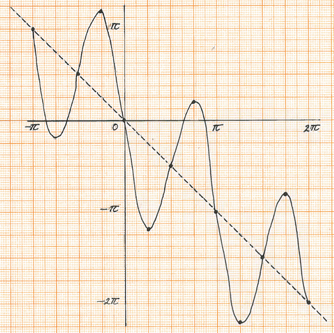
  • (f) y =  − x + 3 sin(2x − π) is obtained by multiplying it by 3, changing the period to π, shifting it to the right by π and finally by plotting this whole function around the line y =  − x. It will look like:

    

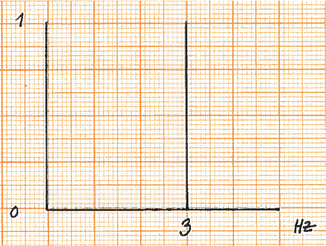
• 3.13. The FFT of

  • (a) a sine with frequency 3 Hz looks like:

    

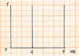
  • (b) the sum of two sines (2 Hz and 5 Hz) looks like:

    

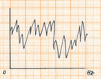
  • (c) white noise looks like (random spectrum):

    

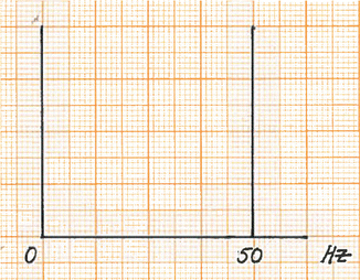
  • (d) 50 Hz noise looks like:

    

Glossary

Accelerometry

Measurement of acceleration using accelerometers (sensor device).

Antisymmetric

In this chapter: a function f for which f(−x) =  − f(x)_.

Cosine

(trigonometric) Ratio between the adjacent edge and the hypothenuse in a right-angled triangle.

Data compression

To represent data such that it occupies less memory.

Deferent

In specific movements described by epicycles and deferents the larger circle that an object moves along.

Delta function

A function that is zero everywhere, except at zero, with an integral of 1 over the entire real domain.

Diadochokinesis

Fast execution of opposite movements, e.g. rotating the hand from palm up to palm down and back.

Enhanced physiological tremor

Tremor that occurs normally, e.g. when fatigued, but stronger in amplitude.

Electroencephalography

Measurement of electrical brain activity using electrodes placed on the scalp.

Electromyography

Measurement of electrical muscle activity using electrodes placed on the skin over a muscle (formally: surface electromyography).

Epicycle

In specific movements described by epicycles and deferents the smaller circle that an object moves along.

Essential tremor

Patients with this type of tremor typically present with action tremor (tremor during posture and/or movements), mostly in the arms, with tremor frequency in the range of 4–12 Hz.

Filtering

Suppression of specific frequencies in a signal.

Function

A mathematical relation, like a recipe, describing how to get from an input to an output.

Functional tremor

Tremor for which no organic cause can be found.

Hypothenuse

Edge opposite the right angle in a right-angled triangle.

Modulo

Modulo(n) expresses equivalence up to a remainder n.

Nyquist frequency

The highest frequency that is still adequately represented in a sampled signal (half the sampling frequency).

Periodic

Repeating itself regularly.

Right-angled (triangle)

A geometric object (triangle) with a right (90°) angle.

Similar (triangles)

Triangles that have the same angles but differ in size.

SI

Système international d’unités (international system of units).

Sine

(trigonometric) Ratio between the opposite edge and the hypothenuse in a right-angled triangle.

Spectrum

Here: representation of a function or signal as a function of frequency, typically resulting from a Fourier transform.

Support

The support of a function is the set of points where the function values are non-zero.

Symmetric

In this chapter: a function f for which f(−x) = f(x)_.

Tangent

(trigonometric) Ratio between the opposite edge and the adjacent edge in a right-angled triangle.

Transfer function

Here: expresses how strongly frequencies are preserved or suppressed by a filter, can vary between 0 and 1.

Tremor

Oscillatory movement of a body part.

Unit circle

Circle with radius one.