Eccentric Axial Force

Abstract

This chapter presents the design methods of reinforced concrete sections subjected to eccentric axial force with their serviceability and resistance verifications. Specific design models are shown for columns and the criteria for nonlinear analysis of frames are presented. In the final section a complete design of an edge column is developed, starting from the stress analysis and following with the pertinent verifications of the critical sections.

The original version of this chapter was revised: For detailed information please see Erratum. The erratum to this chapter is available at 10.1007/978-3-319-52033-9_11

Appendices

Appendix: Eccentric Axial Force

.

Chart 6.1: Eccentric Axial Force: Elastic Design––Formulas

RC Sections subject to combined tension/compression and uniaxial bending.

Symbols

N _Ek :

characteristic value of the applied axial force (positive in compression)

M _Ek :

characteristic value of applied bending moment

A _s :

area of the reinforcement in tension

$A_{\text{s}}^{\prime }$ :

area of the reinforcement in compression

A _t = A _s + $A_{\text{s}}^{\prime }$ :

total reinforcement area

y _o :

position of the design axis

b :

width of the edge in compression

h :

total depth of the section (see figures)

d :

effective depth

d′:

concrete cover of the reinforcement in compression

ρ _s = A _s/(bh):

geometric reinforcement ratio in tension

$\rho_{\text{s}}^{\prime }$ = $A_{\text{s}}^{\prime }$ /bd :

geometric reinforcement ratio in compression

α _e = E _s/E _c :

ratio of elastic moduli (see Chart 2.3)

ψ _s = α _e ρ _s :

elastic reinforcement ratio in tension

$\psi_{\text{s}}^{\prime }$ = α _e $\rho_{\text{s}}^{\prime }$ :

elastic reinforcement ratio in compression

ψ _t = ψ _s + $\psi_{\text{s}}^{\prime }$ :

total elastic reinforcement ratio

σ _c :

maximum compressive stress in concrete

$\sigma_{\text{c}}^{\prime }$ :

maximum tensile stress in concrete

σ _s :

stress in the reinforcement in tension

see also Charts 2.2 and 2.3.

Serviceability Verifications in Phase I

(uncracked section––see figure)

Compression with small eccentricity

$$ \begin{aligned} {\sigma }_{\text{c}} & = \frac{{{N}_{\text{Ek}} }}{{{A}_{\text{i}} }} + \frac{{{M}_{\text{Ek}}^{\prime } }}{{{I}_{\text{i}} }}{y}_{\text{c}} \le {\bar{\sigma }}_{\text{c}} \\ {\sigma }_{\text{G}} & = \frac{{{N}_{\text{Ek}} }}{{{A}_{\text{i}} }} \le 0.7{\bar{\sigma }}_{\text{c}} \\ \end{aligned} $$

with

$$ A_{\text{b}} = bt \qquad A_{\text{w}} = b_{\text{w}} h_{\text{w}} \qquad h_{\text{w}} = h - t $$

$$ \begin{aligned} A_{\text{i}} & = A_{\text{b}} + A_{\text{w}} + \alpha_{\text{e}} A_{\text{s}} + \alpha_{\text{e}} A_{\text{s}}^{\prime } \\ S_{i} & = A_{\text{b}} t/2 + A_{\text{w}} \left( {t + h_{\text{w}} /2} \right) + \alpha_{\text{e}} A_{\text{s}} d + \alpha_{\text{e}} A_{\text{s}}^{\prime } d^{\prime } \\ y_{\text{c}} & = S_{i} /A_{i} \qquad\quad\, y_{\text{c}}^{\prime } = h - y_{\text{c}} \\ y_{\text{s}} & = d - y_{\text{c}} \qquad\quad y_{\text{s}}^{\prime } = y_{\text{c}} - d^{\prime } \\ y_{\text{b}} & = y_{\text{c}} - t/2\qquad y_{\text{w}} = t + h_{\text{w}} /2 - y_{\text{c}} \\ I_{i} & = A_{\text{b}} \left( {t^{2} /12 + y_{\text{b}}^{2} } \right) + A_{\text{w}} \left( {h_{\text{w}}^{2} /12 + y_{\text{w}}^{2} } \right) + \alpha_{\text{e}} A_{\text{s}} y_{\text{s}}^{2} + \alpha_{\text{e}} A_{\text{s}}^{\prime } y_{\text{s}}^{\prime 2} \\ M_{\text{Ek}}^{\prime } & = M_{\text{Ek}} - N_{\text{Ek}} \left( {y_{\text{o}} - y_{\text{c}} } \right) \\ \end{aligned} $$

(for the rectangular section, set t = h)

Generic combined axial force and bending

$$ \begin{aligned} & \sigma_{\text{c}}^{\prime } = \frac{{N_{\text{Ek}} }}{{A_{i} }} + \frac{{M_{\text{Ek}}^{\prime } }}{{I_{i} }}y_{\text{c}}^{\prime } \quad \left( {{\text{positive}}\,{\text{in}}\,{\text{tension}}} \right) \\ & \left( {\sigma_{\text{s}} = - \alpha_{\text{e}} \frac{{N_{\text{Ek}} }}{{A_{i} }} + \alpha_{\text{e}} \frac{{M_{\text{Ek}} }}{{I_{i} }}y_{\text{s}} } \right) \\ \end{aligned} $$

for the verification at the cracking limit:

$$ {\sigma }_{\text{c}}^{\prime } \le 1.3{f}_{\text{ctk}} \quad \left( { = {\bar{\sigma }}_{\text{ct}}^{\prime } \,{\text{with}}\,{\beta } = 1.3 {\text{---}} {\text{see}}\,{\text{Chart}}\,2.2} \right) $$

Serviceability Verifications in Phase II

(cracked section under combined compression and bending)

Rectangular unreinforced section

$$ \begin{aligned} {e} & = {M}_{Ek} /{N}_{\text{Ek}} \quad \left( {{h}/6 \le {e} < {h}/2} \right) \\ {\sigma }_{\text{c}} & = \frac{{2{N}_{\text{Ek}} }}{bx} \le {\bar{\sigma }}_{\text{c}} \\ \end{aligned} $$

with

$$ x = 3\left( {y_{\text{o}} - e} \right) $$

Rectangular section—double reinforcement

(see figure)

$$ \begin{aligned} {\sigma }_{\text{c}} & = \frac{{{N}_{\text{Ek}} }}{{{A}_{i} }} + \frac{{{M}_{\text{Ek}}^{\prime } }}{{{I}_{i} }}{y}_{\text{c}} \le {\bar{\sigma }}_{\text{c}} \quad \left( {\text{compression}} \right) \\ {\sigma }_{\text{s}} & = - {\alpha }_{\text{e}} \frac{{{N}_{\text{Ek}} }}{{{A}_{\text{i}} }} + {\alpha }_{\text{e}} \frac{{{M}_{\text{Ek}}^{\prime } }}{{{I}_{i} }}{y}_{\text{s}} \le {\bar{\sigma }}_{\text{s}} \quad \left( {{\text{tension}}\,{\text{see}}\,{\text{also}}\,{\text{Table}}\, 2.16} \right) \\ \end{aligned} $$

with

$$ \begin{aligned} A_{i} & = bx + \alpha_{\text{e}} A_{\text{s}} + \alpha_{\text{e}} A_{\text{s}}^{\prime } \\ S_{i} & = bx^{2} /2 + \alpha_{\text{e}} A_{\text{s}} d + \alpha_{\text{e}} A_{\text{s}}^{\prime } d^{\prime } \\ y_{\text{c}} & = S_{i} /A_{i} \\ y_{\text{s}} & = d - y_{\text{c}} \quad y_{\text{s}}^{\prime } = y_{\text{c}} - d^{\prime } \\ I_{i} & = bx\left[ {\frac{{x^{2} }}{12} + \left( {y_{\text{c}} - \frac{x}{2}} \right)^{2} } \right] + \alpha_{\text{e}} A_{\text{s}} y_{\text{s}}^{2} + \alpha_{\text{e}} A_{\text{s}}^{\prime } y_{\text{s}}^{\prime 2} \\ M_{\text{Ek}}^{\prime } & = M_{\text{Ek}} - N_{\text{Ek}} \left( {y_{\text{o}} - y_{\text{c}} } \right) \\ \end{aligned} $$

whereas the neutral axis can be deduced from the equation

$$ \xi^{3} + 3\delta_{\text{o}} \xi^{2} + 6\left( {\psi_{\text{s}} \delta_{\text{s}} + \psi_{\text{s}}^{\prime } \delta_{\text{s}}^{\prime } } \right)\xi - 6\left( {\psi_{\text{s}} \delta_{\text{s}} \delta + \psi_{\text{s}}^{\prime } \delta_{\text{s}}^{\prime } \delta^{\prime } } \right) = 0 $$

where it has been set:

$$ \begin{array}{*{20}c} {x = \xi h} \hfill & {\left( { < h} \right)} \hfill \\ {d_{\text{o}} = e - y_{\text{o}} } \hfill & {e = M_{\text{Ek}} /N_{\text{Ek}} } \hfill \\ {\delta_{\text{o}} = d_{\text{o}} /h} \hfill & {\delta^{\prime } = d^{\prime } /h} \hfill \\ {\delta_{\text{s}} = \delta + \delta_{\text{o}} } \hfill & {\delta_{\text{s}}^{\prime } = \delta^{\prime } + \delta_{\text{o}} } \hfill \\ \end{array} $$

T-Section––double reinforcement

(see figure)

$$ \begin{aligned} {\sigma }_{\text{c}} & = \frac{{{N}_{\text{Ek}} }}{{{A}_{i} }} + \frac{{{M}_{\text{Ek}}^{\prime } }}{{{I}_{i} }}{y}_{\text{c}} \le {\bar{\sigma }}_{\text{c}} \quad {\text{compression}} \\ {\sigma }_{\text{s}} & = {\alpha }_{\text{e}} \frac{{{N}_{\text{Ek}} }}{{{A}_{i} }} + {\alpha }_{\text{e}} \frac{{{M}_{\text{Ek}}^{\prime } }}{{{I}_{i} }}{y}_{\text{s}} \le {\bar{\sigma }}_{\text{s}} \quad \left( {{\text{tension}}\,{\text{see}}\,{\text{also}}\,{\text{Table}}\, 2. 1 6} \right) \\ \end{aligned} $$

with $\left( {{\text{a}} = {\text{b}} - {\text{b}}_{\text{w}} ,\,{\text{y}} = {\text{x}} - {\text{t}}} \right)$:

$$ \begin{aligned} A_{i} & = b_{\text{w}} x + at + \alpha_{\text{e}} A_{\text{s}} + \alpha_{\text{e}} A_{\text{s}}^{\prime } \\ S_{i} & = b_{\text{w}} x^{2} /2 + at^{2} /2 + \alpha_{\text{e}} A_{\text{s}} d - \alpha_{\text{e}} A_{\text{s}}^{\prime } d^{\prime } \\ y_{\text{c}} & = S_{i} /A_{i} \\ y_{x} & = y_{\text{c}} - x/2\quad y_{\text{t}} = y_{\text{c}} - t/2 \\ y_{\text{s}} & = d - y_{\text{c}} \quad y_{\text{s}}^{\prime } = y_{\text{c}} - d^{\prime } \\ I_{i} & = bx\left( {x^{2} /12 + y_{x}^{2} } \right) + at\left( {t^{2} /12 + y_{\text{t}}^{2} } \right) + \alpha_{\text{e}} A_{\text{s}} y_{\text{s}}^{2} + \alpha_{\text{e}} A_{\text{s}}^{\prime } y_{\text{s}}^{\prime 2} \\ M_{\text{Ek}}^{\prime } & = M_{\text{Ek}} - N_{\text{Ek}} \left( {y_{\text{o}} - y_{\text{c}} } \right) = N_{\text{Ek}} \left( {d_{\text{o}} + y_{\text{c}} } \right) \\ \end{aligned} $$

whereas the neutral axis can be deduced from the equation

$$ \begin{aligned} \xi^{3} - 3\delta_{\text{o}} \xi^{2} & + \frac{3}{\beta }\left[ {\alpha \tau \left( {2\delta_{\text{o}} + \tau } \right) + 2\left( {\psi_{\text{s}} \delta_{\text{s}} + \psi_{\text{s}}^{\prime } \delta_{\text{s}}^{\prime } } \right)} \right]\xi + \\ & - \frac{1}{\beta }\left[ {\alpha \tau^{2} \left( {3\delta_{\text{o}} + 2\tau } \right) + 6\left( {\psi_{\text{s}} \delta_{\text{s}} \delta + \psi_{\text{s}}^{\prime } \delta_{\text{s}}^{\prime } \delta^{\prime} } \right)} \right] = 0 \\ \end{aligned} $$

where it has been set (t < x < h):

$$ \begin{array}{*{20}c} {x = \xi h} \hfill & {\tau = t/d} \hfill \\ {\beta = b_{\text{w}} /b} \hfill & {\alpha = 1 - \beta } \hfill \\ {d_{\text{o}} = e - y_{\text{o}} } \hfill & {e = M_{\text{Ek}} /N_{\text{Ek}} } \hfill \\ {\delta_{\text{o}} = d_{\text{o}} /h} \hfill & {\delta^{\prime } = d^{\prime } /h\quad \delta = d/h} \hfill \\ {\delta_{\text{s}} = \delta + \delta_{\text{o}} } \hfill & {\delta_{\text{s}}^{\prime } = \delta^{\prime } + \delta_{\text{o}} } \hfill \\ \end{array} $$

Combined Tension and Bending in Phase II

(cracked section––N_Ek positive in tension)

Entirely cracked section

$$ \begin{aligned} & {\sigma }_{\text{s}} = \frac{1}{{{y}_{\text{t}} {A}_{\text{s}} }}\left[ {{N}_{\text{Ek}} {d}_{\text{s}}^{\prime } + {M}_{\text{Ek}} } \right] \le {\bar{\sigma }}_{\text{s}} \quad \left( {{\text{tension}}\,{\text{see}}\,{\text{also}}\,{\text{Table}}\,2.16} \right) \\ & \left( {{\sigma }_{\text{s}}^{\prime } = \frac{1}{{{y}_{\text{t}} {A}_{\text{s}}^{\prime } }}\left[ {{N}_{\text{Ek}} {d}_{\text{s}} - {M}_{\text{Ek}} } \right]} \right) \\ \end{aligned} $$

with

$$ \begin{aligned} y_{\text{s}} & = \frac{{A_{\text{s}}^{\prime } }}{{A_{\text{s}} + A_{\text{s}}^{\prime } }}y_{\text{t}} \quad y_{\text{s}}^{\prime } = \frac{{A_{\text{s}} }}{{A_{\text{s}} + A_{\text{s}}^{\prime } }}y_{\text{t}} \\ y_{\text{t}} & = d - d^{\prime } \\ d_{\text{s}} & = d - y_{\text{o}} \quad d_{\text{s}}^{\prime } = y_{\text{o}} - d^{\prime } \\ \end{aligned} $$

Rectangular cracked section

(see figure)

$$ \begin{aligned} {\sigma }_{\text{c}} & = \frac{{{N}_{\text{Ek}} }}{{{A}_{i} }} + \frac{{{M}_{\text{Ek}}^{\prime } }}{{{I}_{i} }}{y}_{\text{c}} \le {\bar{\sigma }}_{\text{c}} \quad {\text{compression}} \\ {\sigma }_{\text{s}} & = - {\alpha }_{\text{e}} \frac{{{N}_{\text{ak}} }}{{{A}_{i} }} + {\alpha }_{\text{e}} \frac{{{M}_{\text{ak}}^{\prime } }}{{{I}_{i} }}{y}_{\text{s}} \le {\bar{\sigma }}_{\text{s}} \quad \left( {{\text{tension}}\,{\text{see}}\,{\text{also}}\,{\text{Table}}\, 2. 1 6} \right) \\ \end{aligned} $$

with A _i , I _i , y _c, y _s, $M_{\text{Ek}}^{\prime }$ calculated similarly to the corresponding section under combined compression and bending, whereas the neutral axis is deduced from the equation

$$ \xi^{3} - 3\delta_{\text{o}} \xi^{2} - 6\left( {\psi_{\text{s}} \delta_{\text{s}} + \psi_{\text{s}}^{\prime } \delta_{\text{s}}^{\prime } } \right)\xi + 6\left( {\psi_{\text{s}} \delta_{\text{s}} \delta + \psi_{\text{s}}^{\prime } \delta_{\text{s}}^{\prime } \delta^{\prime } } \right) = 0 $$

where it has been set:

$$ \begin{array}{*{20}c} {x = \xi h} \hfill & {\left( { > 0} \right)} \hfill \\ {d_{\text{o}} = e + y_{\text{o}} } \hfill & {e = M_{\text{Ek}} /N_{\text{Ek}} } \hfill \\ {\delta_{\text{o}} = d_{\text{o}} /h} \hfill & {\delta^{\prime } = d^{\prime } /h\quad \delta = d/h} \hfill \\ {\delta_{\text{s}} = \delta_{\text{o}} - \delta } \hfill & {\delta_{s}^{\prime } = \delta_{\text{o}} - \delta^{\prime } } \hfill \\ \end{array} $$

T-shaped cracked section

(see figure)

$$ \begin{aligned} {\sigma }_{\text{c}} & = \frac{{{N}_{\text{Ek}} }}{{{A}_{\text{i}} }} + \frac{{{M}_{\text{Ek}}^{\prime } }}{{{I}_{i} }}{y}_{\text{c}} \le {\bar{\sigma }}_{\text{c}} \quad ({\text{compression}}) \\ {\sigma }_{\text{s}} & = - {\alpha }_{\text{e}} \frac{{{N}_{\text{Ek}} }}{{{A}_{i} }} + {\alpha }_{\text{e}} \frac{{{M}_{\text{Ek}}^{\prime } }}{{{I}_{i} }}{y}_{\text{s}} \le {\bar{\sigma }}_{\text{s}} \quad \left( {{\text{tension}}\,{\text{see}}\,{\text{also}}\,{\text{Table}}\, 2. 1 6} \right) \\ \end{aligned} $$

with A _i , I _i , y _c, y _s, $M_{\text{Ek}}^{\prime }$ calculated similarly to the corresponding section under combined compression and bending, whereas the neutral axis is deduced from the equation

$$ \begin{aligned} \xi^{3} - 3\delta_{\text{o}} \xi^{2} & - \frac{3}{\beta }\left[ {\alpha \tau \left( {2\delta_{\text{o}} - \tau } \right) + 2\left( {\psi_{\text{s}} \delta_{\text{s}} + \psi_{\text{s}}^{\prime } \delta_{\text{s}}^{\prime } } \right)} \right]\xi + \\ & + \frac{1}{\beta }\left[ {\alpha \tau^{2} \left( {3\delta_{\text{o}} - 2\tau } \right) + 6\left( {\psi_{\text{s}} \delta_{\text{s}} \delta + \psi_{\text{s}}^{\prime } \delta_{\text{s}}^{\prime } \delta } \right)} \right] = 0 \\ \end{aligned} $$

where it has been set (t < x < h):

$$ \begin{array}{*{20}c} {x = \xi h} \hfill & {\tau = t/h} \hfill \\ {\alpha = a/b} \hfill & {\beta = b_{\text{w}} /b} \hfill \\ {d_{\text{o}} = e + y_{\text{o}} } \hfill & {e = M_{\text{Ek}} /N_{\text{Ek}} } \hfill \\ {\delta_{\text{o}} = d_{\text{o}} /h} \hfill & {\delta^{\prime } = d^{\prime } /h\quad \delta = d/h} \hfill \\ {\delta_{\text{s}} = \delta_{\text{o}} - \delta } \hfill & {\delta_{\text{s}}^{\prime } = \delta_{\text{o}} - \delta^{\prime } } \hfill \\ \end{array} $$

Chart 6.2: Combined Axial Force and Uniaxial Bending: Resistance Design––Formulas

RC sections subject to combined compression/tension and uniaxial bending. Unless stated otherwise, the indefinite elastic-perfectly plastic σ–ε model has been assumed (model of Fig. 1.30a) for the reinforcement steel.

Symbols

N _Ed :

design value of the applied axial force

M _Ed :

design value of the applied bending moment

M _Rd :

design value of the resisting bending moment

r = f _yd/f _cd :

strength ratio

ω _s = rρ _s :

mechanical reinforcement ratio in tension

$\omega_{\text{s}}^{\prime } = r\rho_{\text{s}}^{\prime }$ :

mechanical reinforcement ratio in compression

ε _yd = f _yd/E _s :

steel yield strain

see also Charts 2.2, 2.3 and 6.1.

Combined Compression and Bending in Phase III

(cracked section with N _Ek positive in compression)

Unreinforced rectangular section

$$ \begin{aligned} & N_{\text{Ed}} \le 0.8f_{\text{cd}} bh \\ & M_{\text{Rd}} = N_{\text{Ed}} e \ge M_{\text{Ed}} \\ \end{aligned} $$

with

$$ \begin{aligned} e & = y_{\text{o}} - \bar{x}/2 \\ \bar{x} & = N_{\text{Ed}} /f_{\text{cd}} b \\ \end{aligned} $$

Rectangular section––double reinforcement

(case with σ _s = f _yd in tension and $\sigma_{\text{s}}^{\prime }$ = f _yd in compression)

$$ {M}_{\text{Rd}} = {f}_{\text{cd}} {{b}\overline{x}}\left( {{y}_{\text{o}} - {\overline{x}}/2} \right) + {f}_{{y{\text{d}}}} {A}_{\text{s}} {y}_{\text{s}} + {f}_{{y{\text{d}}}} {A}_{\text{s}}^{\prime } {y}_{\text{s}}^{\prime } \ge {M}_{\text{Ed}} $$

with

$$ \begin{aligned} \bar{x} & = \left( {N_{\text{Ed}} + f_{{y{\text{d}}}} A_{s} - f_{{y{\text{d}}}} A_{\text{s}}^{\prime } } \right)/f_{\text{cd}} b \\ y_{\text{s}} & = d - y_{\text{o}} \quad y_{\text{s}}^{\prime } = y_{\text{o}} - d^{\prime } \\ \end{aligned} $$

Rectangular section––double reinforcement

(case with σ _s < f _yd in tension and $\sigma_{\text{s}}^{\prime }$ = f _yd in compression)

$$ \begin{aligned} & {M}_{\text{Rd}} = {f}_{\text{cd}} {{b} \overline{x}}\left( {{y}_{\text{o}} - {\overline{x}}/2} \right) + {\sigma }_{s} {A}_{\text{s}} {y}_{\text{s}} + {f}_{{y{\text{d}}}} {A}_{\text{s}}^{\prime } {y}_{\text{s}}^{\prime } \ge {M}_{\text{Ed}} \\ & \left( {{N}_{\text{Ed}} \le 0.8{f}_{\text{cd}} {bh} + {f}_{{y{\text{d}}}} {A}_{\text{s}} + {f}_{{y{\text{d}}}} {A}_{\text{s}}^{\prime } } \right) \\ \end{aligned} $$

with (ε _cu = 0.0035):

$$ \begin{aligned} \bar{x} & = \frac{h}{2}\left\{ {\left( {\nu_{\text{o}} - \alpha_{\text{o}} \omega_{\text{s}} - \omega_{\text{s}}^{\prime } } \right) + \sqrt {\left( {\nu_{\text{o}} - \alpha_{\text{o}} \omega_{\text{s}} - \omega_{\text{s}}^{\prime } } \right)^{2} + 3.2\alpha_{\text{o}} \omega_{\text{s}} \delta } } \right\} \\ \alpha_{\text{o}} & = \varepsilon_{\text{cu}} /\varepsilon_{{y{\text{d}}}} \quad \nu_{o} = N_{\text{Ed}} /\left( {f_{\text{cd}} bh} \right) \\ \sigma_{\text{s}} & = E_{\text{s}} \frac{{0.8d - \bar{x}}}{{\bar{x}}}\varepsilon_{\text{cu}} \le f_{{y{\text{d}}}} \quad {\text{di}}\,{\text{tension}} \\ \end{aligned} $$

Rectangular section––double reinforcement

(case with σ _s = f _yd in tension and $\sigma_{s}^{\prime }$ < f _yd in compression)

$$ {M}_{\text{Rd}} = {f}_{\text{cd}} {{b} \overline{x}}\left( {{y}_{\text{o}} - {\overline{x}}/2} \right) + {f}_{{y{\text{d}}}} {A}_{\text{s}} {y}_{\text{s}} - {\sigma }_{\text{s}}^{\prime } {A}_{\text{s}}^{\prime } {y}_{\text{s}}^{\prime } \ge {M}_{\text{Ed}} $$

with (ε _cu = 0.0035 and δ′ = d′/h):

$$ \begin{aligned} \bar{x} & = \frac{h}{2}\left\{ {\left( {\nu_{\text{o}} - \omega_{\text{s}} - \alpha_{\text{o}} \omega_{\text{s}}^{\prime } } \right) + \sqrt {\left( {\nu_{\text{o}} - \omega_{\text{s}} - \alpha_{\text{o}} \omega_{\text{s}}^{\prime } } \right)^{2} + 3.2\alpha_{\text{o}} \omega_{\text{s}}^{\prime } \delta^{\prime } } } \right\} \\ \alpha_{\text{o}} & = \varepsilon_{\text{cu}} /\varepsilon_{{y{\text{d}}}} \quad \nu_{\text{o}} = \frac{{N_{\text{Ed}} }}{{bhf_{\text{cd}} }} \\ \sigma_{\text{s}}^{\prime } & = E_{\text{s}} \frac{{\bar{x} - 0.8d^{\prime } }}{{\bar{x}}}\varepsilon_{\text{cu}} \le f_{{y{\text{d}}}} \quad {\text{in}}\,{\text{compression}} \\ \end{aligned} $$

T-shaped section––double reinforcement

(case with σ _s = f _yd in tension and $\sigma_{\text{s}}^{\prime }$ = f _yd in compression)

$$ M_{\text{Rd}} = f_{\text{cd}} bt\left( {y_{\text{o}} - t/2} \right) + f_{\text{cd}} b_{\text{w}} \bar{y}\left( {y_{\text{o}} - t - \bar{y}/2} \right) + f_{{y{\text{d}}}} A_{\text{s}} y_{\text{s}} + f_{{y{\text{d}}}} A_{\text{s}}^{\prime } y_{\text{s}}^{\prime } \ge M_{\text{Ed}} $$

with

$$ \begin{aligned} {\bar{\text{y}}} & = \frac{{N_{\text{Ed}} + {\text{f}}_{\text{yd}} {\text{A}}_{\text{s}} - {\text{f}}_{\text{yd}} {\text{A}}_{\text{s}}^{\prime } }}{{{\text{f}}_{\text{cd}} {\text{b}}_{\text{w}} }} - \frac{\text{t}}{\beta }\left( { \ge 0} \right) \\ \beta & = {{b}}_{\text{w}} /{{b}}\quad \left( {{\bar{{x}}} = {{t}} + {\bar{{y}}}} \right) \\ \end{aligned} $$

T-shaped section––double reinforcement

(case with σ _s < f _yd in tension and $\sigma_{\text{s}}^{\prime }$ = f _yd in compression)

$$ M_{\text{Rd}} = f_{\text{cd}} bt\left( {y_{\text{o}} - t/2} \right) + f_{\text{cd}} b_{\text{w}} \bar{y}\left( {y_{\text{o}} - t - \bar{y}/2} \right) + \sigma_{\text{s}} A_{\text{s}} y_{\text{s}} + f_{{y{\text{d}}}} A_{\text{s}}^{\prime } y_{\text{s}}^{\prime } \ge M_{\text{Ed}} $$

with (ε _cu = 0.0035 and δ = d/h):

$$ \begin{aligned} \overline{x} & = \frac{h}{{2{\beta }}}\left\{ {\left( {{\nu }_{\text{o}} - {\alpha }_{\text{o}} {\omega }_{\text{s}} - {\omega }_{\text{s}}^{\prime } - {\alpha \tau }} \right)} \right. + \\ & \left. {\quad + \sqrt {\left( {{\nu }_{\text{o}} - {\alpha }_{\text{o}} {\omega }_{\text{s}} - {\omega }_{\text{s}}^{\prime } - {\alpha \tau }} \right)^{2} + 3.2{\alpha }_{\text{o}} {\beta \omega }_{\text{s}} {\delta }} } \right\} \\ \end{aligned} $$

$$ \begin{array}{*{20}c} {\alpha_{\text{o}} = \varepsilon_{\text{cu}} /\varepsilon_{{y{\text{d}}}} } \hfill & {\nu_{\text{o}} = \frac{{N_{\text{Ed}} }}{{bhf_{\text{cd}} }}} \hfill \\ {\beta = b_{\text{w}} /b} \hfill & {\alpha = 1 - \beta } \hfill \\ {\bar{y} = \bar{x} - t\quad \left( { > 0} \right)} \hfill & {\tau = t/h} \hfill \\ \end{array} $$

Rectangular section––double reinforcement

Finite bilinear model with hardening (Fig. 1.30—model A):

$$ \begin{aligned} \varepsilon_{\text{ud}} & = 0.9\varepsilon_{\text{uk}} \quad \varepsilon_{{y{\text{d}}}} = f_{{y{\text{d}}}} /E_{\text{s}} \\ E_{1} & = \left( {f_{\text{td}} - f_{{y{\text{d}}}} } \right)/\left( {\varepsilon_{\text{uk}} - \varepsilon_{{y{\text{d}}}} } \right) \\ f_{\text{td}}^{\prime } & = f_{{y{\text{d}}}} + E_{1} /\left( {\varepsilon_{\text{uk}} - \varepsilon_{{y{\text{d}}}} } \right) \\ \end{aligned} $$

For B450C steel (see Table 1.17)

$$ \begin{aligned} \varepsilon_{\text{ud}} & = 6.75\% \quad \quad \varepsilon_{\text{yd}} = 0.19\% \\ E_{1} & = 1068\,{\text{N}}/{\text{mm}}^{2} \quad f_{\text{td}}^{\prime } = 461\,{\text{N}}/{\text{mm}}^{2} \\ \end{aligned} $$

with f _yd ≤ σ _s ≤ $f_{\text{td}}^{\prime }$ and f _yd ≤ $\sigma_{\text{s}}^{\prime }$ ≤ $f_{\text{td}}^{\prime }$

$$ \begin{aligned} {M}_{\text{Rd}} & = {f}_{\text{cd}} {b}\overline{x} \left( {{y}_{\text{o}} - \overline{x} /2} \right) + {A}_{\text{s}}^{\prime } {f}_{{y{\text{d}}}} \left[ {1 + {\alpha }\left( {\frac{{\overline{x} - {\beta }_{\text{o}} {d}^{\prime } }}{{\overline{x} }}{\alpha }_{\text{o}} - 1} \right)} \right]\left( {{y}_{\text{o}} - {d}^{\prime } } \right) + \\ & \quad + {A}_{\text{s}} {f}_{{y{\text{d}}}} \left[ {1 + {\alpha }\left( {\frac{{{\beta }_{\text{o}} {d} - \overline{x} }}{{\overline{x} }}{\alpha }_{\text{o}} - 1} \right)} \right]\left( {{d} - {y}_{\text{o}} } \right) \\ \end{aligned} $$

$$ \begin{aligned} \bar{x} & = \frac{h}{2}c\left\{ {1 + \sqrt {1 + 4a\beta_{\text{o}} /c^{2} } } \right\}\qquad \beta_{\text{o}} = 0.8 \\ a & = \alpha \alpha_{\text{o}} \left( {\omega_{\text{s}} d/h + \omega_{\text{s}}^{\prime } d^{\prime } /h} \right) \\ c & = \omega_{\text{s}} \left[ {1 - \alpha \left( {1 + \alpha_{\text{o}} } \right)} \right] - \omega_{\text{s}}^{\prime } \left[ {1 - \alpha \left( {1 - \alpha_{\text{o}} } \right)} \right] + \nu_{\text{o}} \\ \nu_{\text{o}} & = \frac{{N_{\text{Ed}} }}{{bhf_{\text{cd}} }}\qquad \alpha_{\text{o}} = \varepsilon_{\text{cu}} /\varepsilon_{{y{\text{d}}}} \qquad \alpha = {E}_{1}/E_{\text{s}} \\ \end{aligned} $$

Combined Tension and Bending in Phase III

(cracked section––double reinforcement with N _Ed positive in tension)

Entirely cracked section

(with σ _s = f _yd in tension and $\sigma_{\text{s}}^{\prime } < f_{{y{\text{d}}}}$ in tension)

$$ M_{\text{Rd}} = f_{{y{\text{d}}}} A_{\text{s}} y_{\text{s}} - \sigma_{\text{s}}^{\prime } A_{\text{s}}^{\prime } y_{\text{s}}^{\prime } \ge M_{\text{Ed}} $$

with

$$ \begin{aligned} \sigma_{\text{s}}^{\prime } & = \frac{{N_{\text{Ed}} - f_{{y{\text{d}}}} A_{\text{s}} }}{{A_{\text{s}}^{\prime } }}\quad {\text{in}}\,{\text{tension}} \\ y_{\text{s}} & = d - y_{\text{o}} \quad y_{\text{s}}^{\prime } = y_{\text{o}} - d^{\prime } \\ \end{aligned} $$

Rectangular cracked section

(case with σ _s = f _yd in tension and $\sigma_{\text{s}}^{\prime } < f_{{y{\text{d}}}}$ in compression)

$$ {M}_{\text{Rd}} = {f}_{\text{cd}} {{b}\overline{x}} ({y}_{\text{o}} - {\overline{x}}/2 ) {\text{ + f}}_{{y{\text{d}}}} {A}_{\text{s}} {y}_{\text{s}} + {f}_{{y{\text{d}}}} {A}_{\text{s}}^{\prime } {y}_{\text{s}}^{\prime } \ge {M}_{\text{Ed}} $$

with

$$ \bar{x} = \left( {f_{{y{\text{d}}}} A_{\text{s}} - f_{{y{\text{d}}}} A_{\text{s}}^{\prime } - N_{\text{Ed}} } \right)/f_{\text{cd}} b $$

Rectangular cracked section

(case with σ _s = f _yd in tension and $\sigma_{\text{s}}^{\prime } < f_{{y{\text{d}}}}$ in compression)

$$ {M}_{\text{Rd}} = {f}_{\text{cd}} {{b} \overline{x}} ( {y}_{\text{o}} - {\overline{x}}/2 ) + {\text{f}}_{{y{\text{d}}}} {A}_{\text{s}} {y}_{\text{s}} + {\sigma }_{\text{s}}^{\prime } {A}_{\text{s}}^{\prime } {y}_{\text{s}}^{\prime } \ge {M}_{\text{Ed}} $$

with (ε _cu = 0.0035 and $\left. {\delta^{\prime } = d^{\prime } /h} \right)$:

$$ \begin{aligned} \bar{x} & = \frac{h}{2}\left\{ {\left( {\omega_{\text{s}} - \alpha_{\text{o}} \omega_{\text{s}}^{\prime } - \nu_{\text{o}} } \right) + \sqrt {\left( {\omega_{\text{s}} - \alpha_{\text{o}} \omega_{\text{s}}^{\prime } - \nu_{\text{o}} } \right)^{2} + 3.2\alpha_{\text{o}} \omega_{\text{s}}^{\prime } \delta^{\prime } } } \right\} \\ \alpha_{\text{o}} & = \varepsilon_{\text{cu}} /\varepsilon_{{y{\text{d}}}} \quad \nu_{\text{o}} = \frac{{N_{\text{Ed}} }}{{bhf_{\text{cd}} }} \\ \sigma_{\text{s}}^{\prime } & = \frac{{\bar{x} - 0.8d^{\prime } }}{{\bar{x}}}\varepsilon_{\text{cu}} \le f_{{y{\text{d}}}} \quad {\text{in}}\,{\text{compression}} \\ \end{aligned} $$

T-shaped section––double reinforcement

(case with σ _s = f _yd in tension and $\sigma_{\text{s}}^{\prime } = f_{{y{\text{d}}}}$ in compression)

$$ {M}_{\text{Rd}} = {f}_{\text{cd}} {bt(y}_{\text{o}} - {t}/2 ) {\text{ + f}}_{cd} {b}_{w} {\overline{y}} ({y}_{\text{o}} - {t} - {\overline{y}}/ 2) + {f}_{{y{\text{d}}}} {A}_{\text{s}} {y}_{\text{s}} + {f}_{{y{\text{d}}}} {A}_{\text{s}}^{\prime } {y}_{\text{s}}^{\prime } \ge {M}_{\text{Ed}} $$

with

$$ \begin{aligned} \overline{y} & = \frac{{f_{{y{\text{d}}}} A_{\text{s}} - f_{{y{\text{d}}}} A_{\text{s}}^{\prime } - N_{\text{Ed}} }}{{f_{\text{cd}} b_{\text{w}} }} - \frac{t}{\beta }\quad ( \ge 0) \\ \beta & = b_{\text{w}} /b\quad (\overline{x} = t + \overline{y} ) \\ \end{aligned} $$

T-shaped section––double reinforcement

(case with σ _s = f _yd in tension and $\sigma_{\text{s}}^{\prime } < f_{{y{\text{d}}}}$ in compression)

$$ M_{\text{Rd}} = f_{\text{cd}} bt(y_{\text{o}} - t/2) + f_{\text{cd}} b_{\text{w}} \overline{y} (y_{\text{o}} - t - \overline{y} /2) + f_{{y{\text{d}}}} A_{\text{s}} y_{\text{s}} + \sigma_{\text{s}}^{\prime } A_{\text{s}}^{\prime } y_{\text{s}}^{\prime } \ge M_{\text{Ed}} $$

with (ε _cu = 0.0035 and $\delta^{\prime } = d^{\prime } /h$):

$$ \begin{aligned} \bar{x} & = \frac{h}{2\beta }\left\{ {\left( {\omega_{\text{s}} - \alpha_{\text{o}} \omega_{\text{s}}^{\prime } - \nu_{\text{o}} - \alpha \tau } \right)} \right. + \\ & \quad + \left. {\sqrt {\left( {\omega_{\text{s}} - \alpha_{\text{o}} \omega_{\text{s}}^{\prime } - \nu_{\text{o}} - \alpha \tau } \right)^{2} + 3.2\alpha_{\text{o}} \beta \omega_{\text{s}}^{\prime } \delta^{\prime } } } \right\} \\ \end{aligned} $$

$$ \begin{aligned} \alpha_{\text{o}} & = \varepsilon_{\text{cu}} /\varepsilon_{{y{\text{d}}}} \quad \nu_{\text{o}} = \frac{{N_{\text{Ed}} }}{{bhf_{\text{cd}} }} \\ \beta & = b_{\text{w}} /b\quad \alpha = 1 - \beta \\ \bar{y} & = \bar{x} - t\quad ( > 0)\quad \quad \tau = t/h \\ \end{aligned} $$

Chart 6.3: Columns Under Combined Compression and Bending: Shear Resistance

RC columns subject to shear and combined compression with variable bending.

Symbols

N _o = N _Ed :

design value of the axial force (in compression)

e = M _Ed/N _o :

eccentricity of the axial force

V _Ed :

design value of the applied shear force

V _Rd :

design value of the resisting shear force

b _w :

column web width

a _w :

unit area of the web reinforcement (orthogonal stirrups)

ρ _w = a _w/b _w :

geometric reinforcement ratio of the web

ω _w = ρ _w f _yd/f _c2 :

mechanical reinforcement ratio of the web

λ _I :

inclination of initial shear cracking

λ _c :

inclination of web transverse compressions

see also Charts 2.2, 2.3, 6.1, 6.2.

Cracked Segments

Where one has, for the stress calculated at the concrete edge in tension, the value

$$ \sigma_{\text{c}}^{\prime } = - \frac{{N_{\text{o}} }}{{A_{i} }} + \frac{{N_{\text{o}} e}}{{I_{i} }}y_{\text{c}}^{\prime } > \beta f_{\text{ctd}} \quad (\beta = 1.3) $$

the shear resistance is to be calculated with reference to the reduced effective depth:

$$ d^{ * } = d - \left( {N_{\text{o}} - f_{{y{\text{d}}}} A_{\text{s}}^{\prime } } \right)/f_{\text{cd}} b $$

with

$$ V_{\text{Rd}} = \hbox{min} (V_{\text{sd}} ,V_{\text{cd}} ) \ge V_{\text{Ed}} $$

where

$$ \begin{aligned} V_{\text{sd}} & = 0.9d^{ * } a_{\text{w}} f_{\text{sd}} \lambda_{\text{c}} \\ V_{\text{cd}} & = 0.9d^{ * } b_{\text{w}} f_{{{\text{c}}2}} \,\lambda_{\text{c}} /\left( {1 + \lambda_{\text{c}}^{2} } \right) \\ \end{aligned} $$

The inclination λ _c should be assumed within the limits

$$ \lambda_{\text{I}} \le \lambda_{\text{c}} \le \lambda_{\hbox{max} } $$

with

$$ \lambda_{\text{I}} = \tau /\sigma_{\text{I}} \quad \lambda_{\hbox{max} } = \lambda_{\text{I}} + 1.5 $$

where

$$ {\tau } \cong \frac{{{V}_{\text{Ek}} }}{{0.7\,{\text{db}}_{\text{w}} }}\quad \quad {\sigma = }\frac{{{ N}_{\text{Ek}} }}{{{A}_{i} }}\quad ( < 0) $$

$$ \sigma_{\text{I}} = \frac{1}{2}\left( {\sigma + \sqrt {\sigma^{2} + 4\tau^{2} } } \right) $$

(see also Chart 4.2 with d ^* in place of d)

Uncracked Segments

Where, for the stress calculated at the concrete edge in tension, one has the value

$$ \sigma_{\text{c}}^{\prime } = - \frac{{N_{\text{o}} }}{{A_{i} }} + \frac{{N_{\text{o}} e}}{{I_{i} }}y_{\text{c}}^{\prime } \le \beta f_{\text{ctd}} \quad (\beta = 1.3) $$

the shear resistance can be calculated with

$$ {V}_{\text{Rd}} = 0.7\,{\text{db}}_{\text{w}} \sqrt {{\bar{\sigma }}_{\text{td}} \left( {{\bar{\sigma }}_{\text{td}} + {\sigma }} \right) }\le {V}_{\text{Ed}} $$

with

$$ \sigma = \frac{{{\rm N}_{\text{o}} }}{{A_{i} }}\quad ( > 0) $$

and with

$$ \begin{aligned} {\bar{\sigma }}_{\text{td}} & { = f}_{\text{ctd}} \quad\quad\quad\quad\quad\quad\quad\,\,\,\, {\text{for}}\,{\sigma \le }{f}_{\text{cd}} /3 \\ {\bar{\sigma }}_{\text{td}} & { = 1.5}(1 - {\sigma /}{f}_{\text{cd}} ){f}_{\text{ctd}} \quad {\text{for}}\,{\sigma > }{f}_{\text{cd}} /3 \\ \end{aligned} $$

It shall always be

$$ N_{\text{Ed}} = N_{\text{o}} < 0.8f_{\text{cd}} A_{\text{c}} + f_{{y{\text{d}}}} A_{\text{t}} $$

where A _t is the total area of the longitudinal reinforcement.

Chart 6.4: Combined Axial Force and Uniaxial Bending: Supplementary Formulas

RC sections subject to combined compression/tension and uniaxial bending.

Symbols

M _ok :

characteristic value of the cracking moment

M _od :

design value of the cracking moment

see also Charts 2.2, 6.1, 6.2.

Cracking Moment

Serviceability verifications

$$ {M}_{\text{ok}} = \left( {{\bar{\sigma }}_{\text{ct}}^{\prime } - {N}_{\text{Ek}} /{A}_{i} } \right){I}_{i} /{y}_{\text{c}}^{\prime } \ge {M}_{\text{Ek}} \quad \left( {{\bar{\sigma }}_{\text{ct}}^{\prime } = {\beta}{f}_{\text{ctk}}} \right) $$

(for f _ctk see Table 1.2)

Resistance verifications

$$ M_{\text{od}} = (\beta f_{\text{ctd}} - N_{\text{Ed}} /A_{i} )I_{i} /y_{\text{c}}^{\prime } \ge M_{\text{Ed}} \quad \left( {\beta = 1.3} \right) $$

(for A _i , I _i , $y_{\text{c}}^{\prime }$ see Chart 6.1 with figure).

Minimum Reinforcement

For the longitudinal reinforcement at the beam edge in tension a minimum reinforcement should be provided to resist the force released by the concrete in tension when cracking occurs, at the characteristic yield limit f _yk. Such force is to be conventionally calculated based on a triangular distribution of stresses with a maximum at the edge in tension equal to the mean value f _ctm of the concrete tensile strength.

For T-shaped sections or similar, it can be set for example:

$$ A_{\text{s}} \ge \frac{1}{2}\left( {y_{\text{c}}^{\prime } + w} \right)b_{\text{w}} f_{\text{ctm}} /f_{{y{\text{k}}}} $$

with

$$ w = \frac{{I_{i} }}{{A_{i} e^{\prime } }}\qquad e^{\prime } = e + (y_{\text{o}} - y_{\text{c}} ) $$

where

$$ e = \frac{{M_{\text{Ek}} }}{{N_{\text{Ek}} }} $$

is the maximum positive (for N _Ek > 0) or negative (for N _Ek < 0) eccentricity foreseen in the use of the structure (see Chart 6.1 and figure).

Columns Under Combined Compression and Bending

For the construction requirements what reported in Chart 2.9 is also valid.

Chart 6.5: Combined Compression and Biaxial Bending––Section with 4 Bars

The following graph shows the resistance curves of RC rectangular sections as the one in the figure. The section is assumed to be subject to biaxial bending referred to the axes yy and zz. The curves have been obtained with ε _yd = 0.2%, ε _cu = 0.35% and with concrete covers c _y  = 0.1a, c _z  = 0.1b. The definitions are:

$$ \begin{array}{*{20}c} {\nu = {\rm N}_{\text{ED}} /abf_{\text{cd}} } \hfill & {{\text{centred}}\,{\text{adimentional}}\,{\text{axial}}\,{\text{force}}} \hfill \\ \end{array} $$

$$ \begin{array}{*{20}c} {M_{{y{\text{d}}}} = \mu_{\text{y}} a^{2} bf_{\text{cd}} } \hfill & {{\text{applied}}\,{\text{moment}}\,{\text{about}}\,yy} \hfill \\ \end{array} $$

$$ \begin{array}{*{20}c} {{\text{M}}_{\text{zd}} = \mu_{\text{z}} {{ab}}^{2} {\text{f}}_{\text{cd}} } \hfill & {{\text{applied}}\,{\text{moment}}\,{\text{about}}\,zz} \hfill \\ \end{array} $$

$$ \begin{array}{*{20}c} {\omega_{\text{t}} = A_{\text{t}} f_{{y{\text{d}}}} /\left( {abf_{\text{cd}} } \right)} \hfill & {{\text{total}}\,{\text{mechanical}}\,{\text{reinforcement}}\,{\text{ratio}}} \hfill \\ \end{array} $$

see also Charts 2.2, 2.3 and 6.12 and Note on Chart 6.8.

How to Read the Graph

Use the sector relative to the given axial force ν. Insert to scale the point of coordinates μ _y , μ _z corresponding to the given moments. Identify the curve $\bar{\omega }_{\text{t}}$ passing through this point (see below). It shall be $\omega_{\text{t}} > \bar{\omega }_{\text{t}}$. In the graphs with eight sectors (for doubly symmetric sections) choose the axes y and z so that μ _y  ≥ μ _z .

Graph 6.6: Combined Biaxial Bending––Section with 8 Bars

Graph 6.7: Combined Biaxial Bending–Peripheral Reinforcement

Graph 6.8: Combined Biaxial Bending––Section with 6 Bars

Note: Given that a constant distribution (‘stress block’) for the compressions in concrete has been assumed, a precautionary coefficient γ _o≥1 has been added to compensate the approximations of the model at the high levels of axial force (v ≥ 0.4). With respect to the exact values, the ones read in the diagrams are therefore reduced by 5 to 10% depending on the different situations.

Graph 6.9: Combined Biaxial Bending––2 Sides Reinforcement

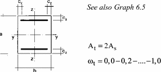
Table 6.10 Combined Biaxial Bending––Analytical Verification

Doubly symmetric reinforced concrete section subject to combined compression and biaxial bending.

Symbols

N _Ed :

design value of the applied axial force

M _Eyd :

design value of the applied moment about y

M _Ezd :

design value of the applied moment about z

y, z :

principal axes of inertia (of symmetry) of the section

M _Ryd :

resisting moment in uniaxial bending about y

M _Rzd :

resisting moment in uniaxial bending about z

Resistance Verification

$$ \left( {\frac{{M_{\text{Eyd}} }}{{M_{\text{Ryd}} }}} \right)^{\alpha } + \left( {\frac{{M_{\text{Ezd}} }}{{M_{\text{Rzd}} }}} \right)^{\alpha } \le 1 $$

For the rectangular sections described above, the exponents α are given in the tables as a function of the following parameters:

$$ \begin{array}{*{20}c} {\nu = \frac{{N_{\text{Ed}} }}{{(abf_{\text{cd}} )}}} \hfill & {{\text{adimentional}}\,{\text{axial}}\,{\text{force}}} \hfill \\ \end{array} $$

$$ \begin{array}{*{20}c} {\omega = \frac{{{\rm A}_{\text{s}} f_{{y{\text{d}}}} }}{{abf_{\text{cd}} }}} \hfill & {{\text{total}}\,{\text{mechanical}}\,{\text{reinforcement}}\,{\text{ratio}}} \hfill \\ \end{array} $$

$$ \begin{array}{*{20}c} {\kappa_{y} = c_{y} /a\quad \kappa_{z} = c_{z} /a} \hfill & {{\text{adimentional}}\,{\text{concrete}}\,{\text{covers}}\,} \hfill \\ \end{array} $$

ν − ω	0.00	0.10	0.20	0.30	0.40	0.50	0.60	0.70	0.80	0.90	1.00
0.00		2.846	2.126	1.875	1.714	1.578	1.499	1.430	1.379	1.335	1.304
0.05	3.503	2.284	1.930	1.728	1.578	1.491	1.420	1.363	1.323	1.303	1.292
0.10	2.620	2.023	1.752	1.589	1.488	1.407	1.352	1.326	1.312	1.299	1.286
0.15	2.198	1.819	1.616	1.486	1.403	1.365	1.342	1.320	1.303	1.289	1.277
0.20	1.978	1.670	1.508	1.435	1.387	1.354	1.325	1.311	1.290	1.272	1.258
0.25	1.829	1.593	1.477	1.405	1.365	1.328	1.300	1.278	1.259	1.245	1.232
0.30	1.728	1.529	1.430	1.366	1.322	1.290	1.266	1.247	1.232	1.219	1.208
0.35	1.652	1.478	1.385	1.326	1.287	1.258	1.237	1.220	1.207	1.196	1.187
0.40	1.599	1.437	1.350	1.296	1.259	1.233	1.214	1.198	1.186	1.176	1.168
0.45	1.566	1.414	1.324	1.269	1.236	1.211	1.192	1.181	1.173	1.165	1.157
0.50	1.549	1.443	1.365	1.310	1.272	1.244	1.223	1.206	1.193	1.183	1.175
0.55	1.544	1.467	1.399	1.346	1.305	1.274	1.249	1.230	1.215	1.204	1.194
0.60	1.556	1.492	1.432	1.382	1.339	1.305	1.278	1.256	1.238	1.224	1.213
0.65	1.582	1.519	1.462	1.416	1.373	1.337	1.307	1.283	1.264	1.247	1.233
0.70	1.627	1.553	1.494	1.446	1.407	1.369	1.337	1.311	1.288	1.269	1.254
0.75	1.698	1.597	1.532	1.478	1.441	1.401	1.368	1.339	1.314	1.293	1.275

Values of α for the section with 8 bars and with κ _y  = κ _z  = κ = 0.10 (δ _max = 2.1%).

ν − ω	0.00	0.10	0.20	0.30	0.40	0.50	0.60	0.70	0.80	0.90	1.00
0.00		2.540	2.072	1.848	1.730	1.644	1.590	1.543	1.509	1.484	1.463
0.05	3.501	2.225	1.901	1.750	1.652	1.588	1.538	1.504	1.477	1.456	1.444
0.10	2.619	2.002	1.781	1.668	1.587	1.533	1.498	1.470	1.453	1.434	1.419
0.15	2.198	1.841	1.690	1.592	1.533	1.493	1.467	1.443	1.424	1.408	1.395
0.20	1.978	1.730	1.608	1.536	1.492	1.458	1.432	1.412	1.396	1.384	1.374
0.25	1.830	1.641	1.543	1.488	1.449	1.421	1.401	1.384	1.372	1.361	1.352
0.30	1.729	1.570	1.493	1.445	1.412	1.389	1.371	1.358	1.348	1.340	1.333
0.35	1.652	1.517	1.448	1.406	1.378	1.359	1.345	1.334	1.326	1.319	1.314
0.40	1.599	1.473	1.407	1.370	1.346	1.330	1.319	1.311	1.304	1.299	1.296
0.45	1.566	1.441	1.377	1.341	1.320	1.305	1.296	1.289	1.284	1.281	1.278
0.50	1.549	1.453	1.386	1.340	1.310	1.289	1.273	1.268	1.265	1.263	1.261
0.55	1.544	1.477	1.420	1.376	1.342	1.317	1.299	1.285	1.275	1.267	1.260
0.60	1.556	1.501	1.451	1.408	1.374	1.347	1.327	1.310	1.297	1.286	1.278
0.65	1.582	1.527	1.479	1.439	1.405	1.376	1.352	1.334	1.319	1.308	1.297
0.70	1.627	1.560	1.509	1.470	1.434	1.404	1.379	1.358	1.342	1.327	1.315
0.75	1.698	1.602	1.543	1.498	1.463	1.431	1.405	1.383	1.365	1.348	1.335

Values of α with peripheral reinforcement and with κ _y  = κ _z  = κ = 0.05 (δ_max = 2.2%).

With a square section symmetric also about the diagonals, set

$$ \begin{array}{*{20}c} {M_{\text{o}} = M_{\text{Ryd}} = M_{\text{Rzd}} } \hfill & {{\text{resisting}}\,{\text{moment}}\,{\text{in}}\,{\text{uniaxial}}\,{\text{bending}}} \hfill \\ {} \hfill & {{\text{about}}\,{\text{a}}\,{\text{median}}\,{\text{axisy}}\,{\text{or}}\,z .} \hfill \\ {M_{\text{Rk}} = M_{{{\text{R}}\eta {\text d}}} = M_{{{\text{R}}\xi {\text{d}}}} } \hfill & {{\text{resisting}}\,{\text{moment}}\,{\text{in}}\,{\text{uniaxial}}\,{\text{bending}}} \hfill \\ {} \hfill & {{\text{about}}\,{\text{a}}\,{\text{diagonal}}\,{\text{axis}}\,{\eta }\,{\text{or}}\,\xi .} \hfill \\ \end{array} $$

one has

$$ \alpha = - \frac{\log 2}{{\lg (M_{\text{k}} /M_{\text{o}} )}} $$

with

$$ M_{\text{k}} = M_{\text{Rk}} /\sqrt 2 $$