
Abstract
In this chapter, the reader will gain knowledge and practical skills about preparing raw clinical data for secondary statistical analysis.
You have full access to this open access chapter, Download chapter PDF
Keywords
FormalPara Learning Objectives-
Understand the requirements for a “clean” database that is “tidy” and ready for use in statistical analysis.
-
Understand the steps of cleaning raw data, integrating data, reducing and reshaping data.
-
Be able to apply basic techniques for dealing with common problems with raw data including missing data inconsistent data, and data from multiple sources.
1 Introduction
Data pre-processing consists of a series of steps to transform raw data derived from data extraction (see Chap. 11) into a “clean” and “tidy” dataset prior to statistical analysis. Research using electronic health records (EHR) often involves the secondary analysis of health records that were collected for clinical and billing (non-study) purposes and placed in a study database via automated processes. Therefore, these databases can have many quality control issues. Pre-processing aims at assessing and improving the quality of data to allow for reliable statistical analysis.
Several distinct steps are involved in pre-processing data. Here are the general steps taken to pre-process data [1]:
-
Data “cleaning”—This step deals with missing data, noise, outliers, and duplicate or incorrect records while minimizing introduction of bias into the database. These methods are explored in detail in Chaps. 13 and 14.
-
“Data integration”—Extracted raw data can come from heterogeneous sources or be in separate datasets. This step reorganizes the various raw datasets into a single dataset that contain all the information required for the desired statistical analyses.
-
“Data transformation”—This step translates and/or scales variables stored in a variety of formats or units in the raw data into formats or units that are more useful for the statistical methods that the researcher wants to use.
-
“Data reduction”—After the dataset has been integrated and transformed, this step removes redundant records and variables, as well as reorganizes the data in an efficient and “tidy” manner for analysis.
Pre-processing is sometimes iterative and may involve repeating this series of steps until the data are satisfactorily organized for the purpose of statistical analysis. During pre-processing, one needs to take care not to accidentally introduce bias by modifying the dataset in ways that will impact the outcome of statistical analyses. Similarly, we must avoid reaching statistically significant results through “trial and error” analyses on differently pre-processed versions of a dataset.
2 Part 1—Theoretical Concepts
2.1 Data Cleaning
Real world data are usually “messy” in the sense that they can be incomplete (e.g. missing data), they can be noisy (e.g. random error or outlier values that deviate from the expected baseline), and they can be inconsistent (e.g. patient age 21 and admission service is neonatal intensive care unit).
The reasons for this are multiple. Missing data can be due to random technical issues with biomonitors, reliance on human data entry, or because some clinical variables are not consistently collected since EHR data were collected for non-study purposes. Similarly, noisy data can be due to faults or technological limitations of instruments during data gathering (e.g. dampening of blood pressure values measured through an arterial line), or because of human error in entry. All the above can also lead to inconsistencies in the data. Bottom line, all of these reasons create the need for meticulous data cleaning steps prior to analysis.
Missing Data
A more detailed discussion regarding missing data will be presented in Chap. 13. Here, we describe three possible ways to deal with missing data [1]:
-
Ignore the record. This method is not very effective, unless the record (observation/row) contains several variables with missing values. This approach is especially problematic when the percentage of missing values per variable varies considerably or when there is a pattern of missing data related to an unrecognized underlying cause such as patient condition on admission.
-
Determine and fill in the missing value manually. In general, this approach is the most accurate but it is also time-consuming and often is not feasible in a large dataset with many missing values.
-
Use an expected value. The missing values can be filled in with predicted values (e.g. using the mean of the available data or some prediction method). It must be underlined that this approach may introduce bias in the data, as the inserted values may be wrong. This method is also useful for comparing and checking the validity of results obtained by ignoring missing records.
Noisy Data
We term noise a random error or variance in an observed variable—a common problem for secondary analyses of EHR data. For example, it is not uncommon for hospitalized patients to have a vital sign or laboratory value far outside of normal parameters due to inadequate (hemolyzed) blood samples, or monitoring leads disconnected by patient movement. Clinicians are often aware of the source of error and can repeat the measurement then ignore the known incorrect outlier value when planning care. However, clinicians cannot remove the erroneous measurement from the medical record in many cases, so it will be captured in the database. A detailed discussion on how to deal with noisy data and outliers is provided in Chap. 14; for now we limit the discussion to some basic guidelines [1].
-
Binning methods. Binning methods smooth a sorted data value by considering their ‘neighborhood’, or values around it. These kinds of approaches to reduce noise, which only consider the neighborhood values, are said to be performing local smoothing.
-
Clustering. Outliers may be detected by clustering, that is by grouping a set of values in such a way that the ones in the same group (i.e., in the same cluster) are more similar to each other than to those in other groups.
-
Machine learning. Data can be smoothed by means of various machine learning approaches. One of the classical methods is the regression analysis, where data are fitted to a specified (often linear) function.
Same as for missing data, human supervision during the process of noise smoothing or outliers detection can be effective but also time-consuming.
Inconsistent Data
There may be inconsistencies or duplications in the data. Some of them may be corrected manually using external references. This is the case, for instance, of errors made at data entry. Knowledge engineering tools may also be used to detect the violation of known data constraints. For example, known functional dependencies among attributes can be used to find values contradicting the functional constraints.
Inconsistencies in EHR result from information being entered into the database by thousands of individual clinicians and hospital staff members, as well as captured from a variety of automated interfaces between the EHR and everything from telemetry monitors to the hospital laboratory. The same information is often entered in different formats by these different sources.
Take, for example, the intravenous administration of 1 g of the antibiotic vancomycin contained in 250 mL of dextrose solution. This single event may be captured in the dataset in several different ways. For one patient this event may be captured from the medication order as the code number (ITEMID in MIMIC) from the formulary for the antibiotic vancomycin with a separate column capturing the dose stored as a numerical variable. However, on another patient the same event could be found in the fluid intake and output records under the code for the IV dextrose solution with an associated free text entered by the provider. This text would be captured in the EHR as, for example “vancomycin 1 g in 250 ml”, saved as a text variable (string, array of characters, etc.) with the possibility of spelling errors or use of nonstandard abbreviations. Clinically these are the exact same event, but in the EHR and hence in the raw data, they are represented differently. This can lead to the same single clinical event not being captured in the study dataset, being captured incorrectly as a different event, or being captured multiple times for a single occurrence.
In order to produce an accurate dataset for analysis, the goal is for each patient to have the same event represented in the same manner for analysis. As such, dealing with inconsistency perfectly would usually have to happen at the data entry or data extraction level. However, as data extraction is imperfect, pre-processing becomes important. Often, correcting for these inconsistencies involves some understanding of how the data of interest would have been captured in the clinical setting and where the data would be stored in the EHR database.
2.2 Data Integration
Data integration is the process of combining data derived from various data sources (such as databases, flat files, etc.) into a consistent dataset. There are a number of issues to consider during data integration related mostly to possible different standards among data sources. For example, certain variables can be referred by means of different IDs in two or more sources.
In the MIMIC database this mainly becomes an issue when some information is entered into the EHR during a different phase in the patient’s care pathway, such as before admission in the emergency department, or from outside records. For example, a patient may have laboratory values taken in the ER before they are admitted to the ICU. In order to have a complete dataset it will be necessary to integrate the patient’s full set of lab values (including those not associated with the same MIMIC ICUSTAY identifier) with the record of that ICU admission without repeating or missing records. Using shared values between datasets (such as a hospital stay identifier or a timestamp in this example) can allow for this to be done accurately.
Once data cleaning and data integration are completed, we obtain one dataset where entries are reliable.
2.3 Data Transformation
There are many possible transformations one might wish to do to raw data values depending on the requirement of the specific statistical analysis planned for a study. The aim is to transform the data values into a format, scale or unit that is more suitable for analysis (e.g. log transform for linear regression modeling). Here are few common possible options:
Normalization
This generally means data for a numerical variable are scaled in order to range between a specified set of values, such as 0–1. For example, scaling each patient’s severity of illness score to between 0 and 1 using the known range of that score in order to compare between patients in a multiple regression analysis.
Aggregation
Two or more values of the same attribute are aggregated into one value. A common example is the transformation of categorical variables where multiple categories can be aggregated into one. One example in MIMIC is to define all surgical patients by assigning a new binary variable to all patients with an ICU service noted to be “SICU” (surgical ICU) or “CSRU” (cardiac surgery ICU).
Generalization
Similar to aggregation, in this case low level attributes are transformed into higher level ones. For example, in the analysis of chronic kidney disease (CKD) patients, instead of using a continuous numerical variable like the patient’s creatinine levels, one could use a variable for CKD stages as defined by accepted guidelines.
2.4 Data Reduction
Complex analysis on large datasets may take a very long time or even be infeasible. The final step of data pre-processing is data reduction, i.e., the process of reducing the input data by means of a more effective representation of the dataset without compromising the integrity of the original data. The objective of this step is to provide a version of the dataset on which the subsequent statistical analysis will be more effective. Data reduction may or may not be lossless. That is the end database may contain all the information of the original database in more efficient format (such as removing redundant records) or it may be that data integrity is maintained but some information is lost when data is transformed and then only represented in the new form (such as multiple values being represented as an average value).
One common MIMIC database example is collapsing the ICD9 codes into broad clinical categories or variables of interest and assigning patients to them. This reduces the dataset from having multiple entries of ICD9 codes, in text format, for a given patient, to having a single entry of a binary variable for an area of interest to the study, such as history of coronary artery disease. Another example would be in the case of using blood pressure as a variable in analysis. An ICU patient will generally have their systolic and diastolic blood pressure monitored continuously via an arterial line or recorded multiple times per hour by an automated blood pressure cuff. This results in hundreds of data points for each of possibly thousands of study patients. Depending on the study aims, it may be necessary to calculate a new variable such as average mean arterial pressure during the first day of ICU admission.
Lastly, as part of more effective organization of datasets, one would also aim to reshape the columns and rows of a dataset so that it conforms with the following 3 rules of a “tidy” dataset [2, 3]:
-
1.
Each variable forms a column
-
2.
Each observation forms a row
-
3.
Each value has its own cell
“Tidy” datasets have the advantage of being more easily visualized and manipulated for later statistical analysis. Datasets exported from MIMIC usually are fairly “tidy” already; therefore, rule 2 is hardly ever broken. However, sometimes there may still be several categorical values within a column even for MIMIC datasets, which breaks rule 1. For example, multiple categories of marital status or ethnicity under the same column. For some analyses, it is useful to split each categorical values of a variable into their own columns. Fortunately though, we do not often have to worry about breaking rule 3 for MIMIC data as there are not often multiple values in a cell. These concepts will become clearer after the MIMIC examples in Sect. 12.3
3 PART 2—Examples of Data Pre-processing in R
There are many tools for doing data pre-processing available, such as R, STATA, SAS, and Python; each differs in the level of programming background required. R is a free tool that is supported by a range of statistical and data manipulation packages. In this section of the chapter, we will go through some examples demonstrating various steps of data pre-processing in R, using data from various MIMIC dataset (SQL extraction codes included). Due to the significant content involved with the data cleaning step of pre-processing, this step will be separately addressed in Chaps. 13 and 14. The examples in this section will deal with some R basics as well as data integration, transformation, and reduction.
3.1 R—The Basics
The most common data output from a MIMIC database query is in the form of ‘comma separated values’ files, with filenames ending in ‘.csv’. This output file format can be selected when exporting the SQL query results from MIMIC database. Besides ‘.csv’ files, R is also able to read in other file formats, such as Excel, SAS, etc., but we will not go into the detail here.
Understanding ‘Data Types’ in R
For many who have used other data analysis software or who have a programming background, you will be familiar with the concept of ‘data types’.
R strictly stores data in several different data types, called ‘classes’:
-
Numeric – e.g. 3.1415, 1.618
-
Integer – e.g. -1, 0, 1, 2, 3
-
Character – e.g. “vancomycin”, “metronidazole”
-
Logical – TRUE, FALSE
-
Factors/categorical – e.g. male or female under variable, gender
R also usually does not allow mixing of data types for a variable, except in a:
-
List – as a one dimensional vector, e.g. c(“vancomycin”, 1.618, “red”)
-
Data-frame – as a two dimensional table with rows (observations) and columns (variables)
Lists and data-frames are treated as their own ‘class’ in R.
Query output from MIMIC commonly will be in the form of data tables with different data types in different columns. Therefore, R usually stores these tables as ‘data-frames’ when they are read into R.
Special Values in R
-
NA – ‘not available’, usually a default placeholder for missing values.
-
NAN – ‘not a number’, only applying to numeric vectors.
-
NULL – ‘empty’ value or set. Often returned by expressions where the value is undefined.
-
Inf – value for ‘infinity’ and only applies to numeric vectors.
Setting Working Directory
This step tells R where to read in the source files.
Command: setwd(“directory_path”)
Example: (If all data files are saved in directory “MIMIC_data_files” on the Desktop)

Reading in .csv Files from MIMIC Query Results
The data read into R is assigned a ‘name’ for reference later on.
Command: set_var_name <- read.csv(“filename.csv”)
Example:

Viewing the Dataset
There are several commands in R that are very useful for getting a ‘feel’ of your datasets and see what they look like before you start manipulating them.
-
View the first and last 2 rows. E.g.:

-
View summary statistics. E.g.:

-
View structure of data set (obs = number of rows). E.g.:

-
Find out the ‘class’ of a variable or dataset. E.g.:

-
View number of rows and column, or alternatively, the dimension of the dataset. E.g.:

-
Calculate length of a variable. E.g.:


Subsetting a Dataset and Adding New Variables/Columns
Aim: Sometimes, it may be useful to look at only some columns or some rows in a dataset/data-frame—this is called subsetting.
Let’s create a simple data-frame to demonstrate basic subsetting and other command functions in R. One simple way to do this is to create each column of the data-frame separately then combine them into a dataframe later. Note the different kinds of data types for the columns/variables created, and beware that R is case-sensitive.
Examples: Note that comments appearing after the hash sign (#) will not be evaluated.

To subset or extract only e.g., weight, we can use either the dollar sign ($) after the dataset, data, or use the square brackets, []. The $ selects column with the column name (without quotation mark in this case). The square brackets [] here selected the column weight by its column number:

Generally one can subset a dataset by specifying the rows and column desired like this: data[row number, column number]. For example:

The square brackets are useful for subsetting multiple columns or rows. Note that it is important to ‘concatenate’, c(), if selecting multiple variables/columns and to use quotation marks when selecting with columns names

To calculate the BMI (weight/height^2) in a new column—there are different ways to do this but here is a simple method:

Let’s create a new column, obese, for BMI > 30, as TRUE or FALSE. This also demonstrates the use of ‘logicals’ in R.

One can also use logical vectors to subset datasets in R. A logical vector, named “ob” here, is created and then we pass it through the square brackets [] to tell R to select only the rows where the condition BMI > 30 is TRUE:

Combining Datasets (Called Data Frames in R)
Aim: Often different variables (columns) of interest in a research question may come from separate MIMIC tables and could have been exported as separate.csv files if they were not merged via SQL queries. For ease of analysis and visualization, it is often desirable to merge these separate data frames in R on their shared ID column(s).
Occasionally, one may also want to attach rows from one data frame after rows from another. In this case, the column names and the number of columns of the two different datasets must be the same.
Examples: In general, there are a couple ways of combining columns and rows from different datasets in R:
-
merge()—This function merges columns on shared ID column(s) between the data frames so the associated rows match up correctly.
Command: merging on one ID column, e.g.:

Command: merging on two ID columns, e.g.:

-
cbind()—This function simply ‘add’ together the columns from two data frames (must have equal number of rows). It does not match up the rows by any identifier.
Command: joining columns. E.g.:

-
rbind()—The function ‘row binds’ the two data frames vertically (must have the same column names).
Command: joining rows. E.g.:

Using Packages in R
There are many packages that make life so much easier when manipulating data in R. They need to be installed on your computer and loaded at the start of your R script before you can call the functions in them. We will introduce examples of of a couple of useful packages later in this chapter.
For now, the command for installing packages is:

The command for loading the package into the R working environment:

Note—there are no quotation marks when loading packages as compared to installing; you will get an error message otherwise.
Getting Help in R
There are various online tutorials and Q&A forums for getting help in R. Stackoverflow, Cran and Quick-R are some good examples. Within the R console, a question mark, ?, followed by the name of the function of interest will bring up the help menu for the function, e.g.

3.2 Data Integration
Aim: This involves combining the separate output datasets exported from separate MIMIC queries into a consistent larger dataset table.
To ensure that the associated observations or rows from the two different datasets match up, the right column ID must be used. In MIMIC, the ID columns could be subject_id, hadm_id, icustay_id, itemid, etc. Hence, knowing the context of what each column ID is used to identify and how they are related to each other is important. For example, subject_id is used to identify each individual patient, so includes their date of birth (DOB), date of death (DOD) and various other clinical detail and laboratory values in MIMIC. Likewise, the hospital admission ID, hadm_id, is used to specifically identify various events and outcomes from an unique hospital admission; and is also in turn associated with the subject_id of the patient who was involved in that particular hospital admission. Tables pulled from MIMIC can have one or more ID columns. The different tables exported from MIMIC may share some ID columns, which allows us to ‘merge’ them together, matching up the rows correctly using the unique ID values in their shared ID columns.
Examples: To demonstrate this with MIMIC data, a simple SQL query is constructed to extract some data, saved as: “population.csv” and “demographics.csv”.
We will these extracted files to show how to merge datasets in R.
-
1.
SQL query:

Note: Remove the -- in front of the SELECT command to run the query.
-
2.
R code: Demonstrating data integration
Set working directory and read data files into R::

Merging pop and demo: Note to get the rows to match up correctly, we need to merge on both the subject_id and hadm_id in this case. This is because each subject/patient could have multiple hadm_id from different hospital admissions during the EHR course of MIMIC database.

As you can see, there are still multiple problems with this merged database, for example, the missing values for ‘marital_status_descr’ column. Dealing with missing data is explored in Chap. 13.
3.3 Data Transformation
Aim: To transform the presentation of data values in some ways so that the new format is more suitable for the subsequent statistical analysis. The main processes involved are normalization, aggregation and generalization (See part 1 for explanation).
Examples: To demonstrate this with a MIMIC database example, let us look at a table generated from the following simple SQL query, which we exported as “comorbidity_scores.csv”.
The SQL query selects all the patient comorbidity information from the mimic2v26.comorbidity_scores table on the condition of (1) being an adult, (2) in his/her first ICU admission, and (3) where the hadm_id is not missing according to the mimic2v26.icustay_detail table.
-
1.
SQL query:

-
2.
R code: Demonstrating data transformation:


Note the ‘class’ or data type of each column/variable and the total number of rows (obs) and columns (variables) in c_scores:

Here we add a column in c_scores to save the overall ELIXHAUSER. The rep() function in this case repeats 0 for nrow(c_scores) times. Function, colnames(), rename the new or last column, [ncol(c_scores)], as “ELIXHAUSER_overall”.

Take a look at the result. Note the new “ELIXHAUSER_overall” column added at the end:

Aggregation Step
Aim: To sum up the values of all the ELIXHAUSER comorbidities across each row. Using a ‘for loop’, for each i-th row entry in column “ELIXHAUSER_overall”, we sum up all the comorbidity scores in that row.

Let’s take a look at the head of the resulting first and last column:

Normalization Step
Aim: Scale values in column ELIXHAUSER_overall to between 0 and 1, i.e. in [0, 1]. Function, max(), finds out the maximum value in column ELIXHAUSER overall. We then re-assign each entry in column ELIXHAUSERoverall as a proportion of the max_score to normalize/scale the column.

We subset and remove all the columns in c_score, except for “subject_id”, “hadm_id”, and “ELIXHAUSER_overall”:

Generalization Step
Aim: Consider only the patient sicker than the average Elixhauser score. The function, which(), return the row numbers (indices) of all the TRUE entries of the logical condition set on c_scores inside the round () brackets, where the condition being the column entry for ELIXHAUSER_overall ≥0.5. We store the row indices information in the vector, ‘sicker’. Then we can use ‘sicker’ to subset c_scores to select only the rows/patients who are ‘sicker’ and store this information in ‘c_score_sicker’.

Saving the results to file: There are several functions that will do this, e.g. write.table() and write.csv(). We will give an example here:

If you check in your working directory/folder, you should see the new “c_score_sicker.csv” file.
3.4 Data Reduction
Aim: To reduce or reshape the input data by means of a more effective representation of the dataset without compromising the integrity of the original data. One element of data reduction is eliminating redundant records while preserving needed data, which we will demonstrate in Example Part 1. The other element involves reshaping the dataset into a “tidy” format, which we will demonstrate in below sections.
Examples Part 1: Eliminating Redundant Records
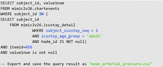
To demonstrate this with a MIMIC database example, we will look at multiple records of non-invasive mean arterial pressure (MAP) for each patient. We will use the records from the following SQL query, which we exported as “mean_arterial_pressure.csv”.
The SQL query selects all the patient subject_id’s and noninvasive mean arterial pressure (MAP) measurements from the mimic2v26.chartevents table on the condition of (1) being an adult, (2) in his/her first ICU admission, and (3) where the hadm_id is not missing according to the mimic2v26.icustay_detail table.
-
1.
SQL query:
-
2.
R code:

There are a variety of methods that can be chosen to aggregate records. In this case we will look at averaging multiple MAP records into a single average MAP for each patient. Other options which may be chosen include using the first recorded value, a minimum or maximum value, etc.
For a basic example, the following code demonstrates data reduction by averaging all of the multiple records of MAP into a single record per patient. The code uses the aggregate() function:

This step averages the MAP values for each distinct subject_id:

Examples Part 2: Reshaping Dataset
Aim: Ideally, we want a “tidy” dataset reorganized in such a way so it follows these 3 rules [2, 3]:
-
1.
Each variable forms a column
-
2.
Each observation forms a row
-
3.
Each value has its own cell
Datasets exported from MIMIC usually are fairly “tidy” already. Therefore, we will construct our own data frame here for ease of demonstration for rule 3. We will also demonstrate how to use some common data tidying packages.
R code: To mirror our own MIMIC dataframe, we construct a dataset with a column of subject_id and a column with a list of diagnoses for the admission.

Note that the dataset above is not “tidy”. There are multiple categorical variables in column “diagnosis”—breaks “tidy” data rule 1. There are multiple values in column “diagnosis”—breaks “tidy” data rule 3.
There are many ways to “tidy” and reshape this dataset. We will show one way to do this by making use of R packages “splitstackshape” [5] and “tidyr” [4] to make reshaping the dataset easier.
R package example 1—“splitstackshape”:
Installing and loading the package into R console.

The function, cSplit(), can split the multiple categorical values in each cell of column “diagnosis” into different columns, “diagnosis_1” and “diagnosis_2”. If the argument, direction, for cSplit() is not specified, then the function splits the original dataset “wide”.

One could possibly keep it as this if one is interested in primary and secondary diagnoses (though it is not strictly “tidy” yet).
Alternatively, if the direction argument is specified as “long”, then cSplit split the function “long” like so:

Note diag3 is still not “tidy” as there are still multiple categorical variables under column diagnosis—but we no longer have multiple values per cell.
R package example 2—“tidyr”:
To further “tidy” the dataset, package “tidyr” is pretty useful.

The aim is to split each categorical variable under column, diagnosis, into their own columns with 1 = having the diagnosis and 0 = not having the diagnosis. To do this we first construct a third column, “yes”, that hold all the 1 values initially (because the function we are going use require a value column that correspond with the multiple categories column we want to ‘spread’ out).

Then we can use the spread function to split each categorical variables into their own columns. The argument, fill = 0, replaces the missing values.

One can see that this dataset is now “tidy”, as it follows all three “tidy” data rules.
4 Conclusion
A variety of quality control issues are common when using raw clinical data collected for non-study purposes. Data pre-processing is an important step in preparing raw data for statistical analysis. Several distinct steps are involved in pre-processing raw data as described in this chapter: cleaning, integration, transformation, and reduction. Throughout the process it is important to understand the choices made in pre-processing steps and how different methods can impact the validity and applicability of study results. In the case of EHR data, such as that in the MIMIC database, pre-processing often requires some understanding of the clinical context under which data were entered in order to guide these pre-processing choices. The objective of all the steps is to arrive at a “clean” and “tidy” dataset suitable for effective statistical analyses while avoiding inadvertent introduction of bias into the data.
Take Home Messages
-
Raw data for secondary analysis is frequently “messy” meaning it is not in a form suitable for statistical analysis; data must be “cleaned” into a valid, complete, and effectively organized “tidy” database that can be analyzed.
-
There are a variety of techniques that can be used to prepare data for analysis, and depending on the methods use, this pre-processing step can introduce bias into a study.
-
The goal of pre-processing data is to prepare the available raw data for analysis without introducing bias by changing the information contained in the data or otherwise influencing end results.
References
Son NH (2006) Data mining course—data cleaning and data preprocessing. Warsaw University. Available at URL http://www.mimuw.edu.pl/~son/datamining/DM/4-preprocess.pdf
Grolemund G (2016) R for data science—data tidying. O’Reilly Media. Available at URL http://garrettgman.github.io/tidying/
Wickham H (2014) J Stat Softw 59(10). Tidy Data. Available at URL http://vita.had.co.nz/papers/tidy-data.pdf
Wickham H (2016) Package ‘tidyr’—easily tidy data with spread() and gather() functions. CRAN. Available at URL https://cran.r-project.org/web/packages/tidyr/tidyr.pdf
Mahto A (2014) Package ‘splitstackshape’—stack and reshape datasets after splitting concatenated values. CRAN. Available at URL https://cran.r-project.org/web/packages/splitstackshape/splitstackshape.pdf
Author information
Authors and Affiliations
Rights and permissions
Open Access This chapter is distributed under the terms of the Creative Commons Attribution-NonCommercial 4.0 International License (http://creativecommons.org/licenses/by-nc/4.0/), which permits any noncommercial use, duplication, adaptation, distribution and reproduction in any medium or format, as long as you give appropriate credit to the original author(s) and the source, a link is provided to the Creative Commons license and any changes made are indicated.
The images or other third party material in this chapter are included in the work’s Creative Commons license, unless indicated otherwise in the credit line; if such material is not included in the work’s Creative Commons license and the respective action is not permitted by statutory regulation, users will need to obtain permission from the license holder to duplicate, adapt or reproduce the material.
Copyright information
© 2016 The Author(s)
About this chapter
Cite this chapter
Malley, B., Ramazzotti, D., Wu, J.Ty. (2016). Data Pre-processing. In: Secondary Analysis of Electronic Health Records. Springer, Cham. https://doi.org/10.1007/978-3-319-43742-2_12
Download citation
DOI: https://doi.org/10.1007/978-3-319-43742-2_12
Published:
Publisher Name: Springer, Cham
Print ISBN: 978-3-319-43740-8
Online ISBN: 978-3-319-43742-2
eBook Packages: MedicineMedicine (R0)