Array Folds Logic

Abstract

We present an extension to the quantifier-free theory of integer arrays which allows us to express counting. The properties expressible in Array Folds Logic (AFL) include statements such as “the first array cell contains the array length,” and “the array contains equally many minimal and maximal elements.” These properties cannot be expressed in quantified fragments of the theory of arrays, nor in the theory of concatenation. Using reduction to counter machines, we show that the satisfiability problem of AFL is PSPACE-complete, and with a natural restriction the complexity decreases to NP. We also show that adding either universal quantifiers or concatenation leads to undecidability.

AFL contains terms that fold a function over an array. We demonstrate that folding, a well-known concept from functional languages, allows us to concisely summarize loops that count over arrays, which occurs frequently in real-life programs. We provide a tool that can discharge proof obligations in AFL, and we demonstrate on practical examples that our decision procedure can solve a broad range of problems in symbolic testing and program verification.

This research was supported in part by the European Research Council (ERC) under grant 267989 (QUAREM) and by the Austrian Science Fund (FWF) under grants S11402-N23 (RiSE and SHiNE) and Z211-N23 (Wittgenstein Award).

1 Introduction

Arrays and lists (or, more generally, sequences) are fundamental data structures both for imperative and functional programs: hardly any real-life program can work without processing sequentially-ordered data. Testing and verification of array- and list-manipulating programs is thus a task of crucial importance. Almost any non-trivial property about these data structures requires some sort of universal quantification; unfortunately, the full first-order theories of arrays and lists are undecidable. This has motivated researches to investigate fragments with restricted quantifier prefixes, and has given rise to numerous logics that can describe interesting properties of sequences, such as partitioning or sortedness. These logics have efficient decision procedures and have been successfully applied to verify some important aspects of programs working with arrays and lists: for example, the correctness of sorting algorithms.

However, an important class of properties, namely, counting over arrays, has eluded researchers’ attention so far. In addition to the examples from the abstract, this includes statements such as “the histogram of the input data satisfies the given distribution,” or “the packet adheres to the requirements of the given type-length-value (TLV) encoding (e.g., of the IPv6 options).” Such properties, though crucial for many applications, cannot be expressed in decidable fragments of the first-order theory of arrays, nor in the decidable extensions of the theory of concatenation.

Fig. 1.

A toy array problem

In this paper we present Array Folds Logic (AFL), which is an extension of the quantifier-free theory of integer arrays. But instead of introducing quantifiers, we introduce counting in the form of $fold$ terms. Folding is a well-known concept in functional languages: as the name suggests, it folds some function over an array, i.e., applies it to every element of the array in sequence, while preserving the intermediate result.

To illustrate the kind of problems we are dealing with, consider the following toy example: given an array, accept it if the number of minimum elements in the array is the same as the number of maximum elements in the array. E.g., the array [1, 2, 7, 4, 1, 3, 7, 5] is accepted (because there are two 1’s and two 7’s), while the array [1, 2, 7, 4, 1, 3, 6, 5] is rejected (because there is only one 7).

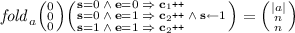
Written in a programming language like C, the problem can be solved by the piece of code shown in Fig. 1a, but such explicit solution cannot express verification conditions for symbolic verification and testing. We can use the quantified theory of arrays mixed with assertions about cardinality of sets, as in Fig. 1b. Unfortunately, such a combination is undecidable (by a reduction from Hilbert’s Tenth Problem: replace $fold$s with cardinalities in the proof of Theorem 2).

The solution we propose is shown in Fig. 1c: in the example formula, the first $fold$ applies a function to array a. The vector in the first parentheses gives initial values for the array index and counter $\mathbf {c}_1$; the function is folded over the array starting from the initial index. Index variable $\mathbf {i}$ is implicit, and it is incremented at each iteration. The function itself is given in the second parentheses, and has two branches. The first branch counts the number of positions with elements equal to $min$ in counter $\mathbf {c}_1$. The second branch $skip$s when the current array element $\mathbf {e}$ is greater than the (guessed, existentially quantified) variable $min$. When $\mathbf {e}< min$, the implicit $break$ statement is executed, and the $fold$ terminates prematurely. The result of the $fold$ is compared to the vector which asserts that the final value of the array index equals to the array size |a| (which means no $break$ was executed), and the final value of $\mathbf {c}_1$ equals to j. The positions where elements are equal to $max$, are counted in the second $fold$, and the equality between these two counts is asserted. The ability to count over arrays with unbounded elements is a unique feature of Array Folds Logic.

This paper makes the following contributions:

1. We define a new logic, called AFL, that can express interesting and non-trivial properties of counting over arrays, which are orthogonal to the properties expressible by other logics. Additionally, AFL can concisely summarize loops with internal branching that traverse arrays and perform counting, enabling verification and symbolic testing of programs with such loops.

2. We show that the satisfiability problem for AFL is $\mathbf {PSPACE}$-complete, and with a natural restriction the complexity decreases to $\mathbf {NP}$. We provide a decision procedure for AFL, which works by a reduction to the emptiness of (symbolic) reversal-bounded counter machines, which in turn reduces to the satisfiability of existential Presburger formulas. We show that adding either universal quantifiers or concatenation leads to undecidability.

3. We implemented tool AFolder [13] that can discharge proof obligations in AFL, and we demonstrate on real-life examples that our decision procedure can solve a broad range of problems in symbolic testing and program verification.

Related Work. Our logic is related to the quantified fragments of the theory of arrays such as [4, 10, 21, 22]. These logics allow restricted quantifier prefixes, and their decision procedures work by rewriting to the (parametric) theories of array indices and elements (Presburger arithmetic being the most common case) [4, 10], or by reduction to flat counter automata with difference bound constraints [21, 22]. An interesting alternative is provided in [35], where the quantification is arbitrary, but array elements must be bounded by a constant given a priori; the decision procedure works by a reduction to WS1S. A separate line of work is presented by the theory combination frameworks of [16, 18], where the quantifier-free theory of arrays is extended by $injective$ predicate and $domain$ function [18], or with $map$ and $constant$-$value$ combinators [16]. The theory of concatenation and its extensions [11, 17, 29] are also related; their decision procedures work by reduction to Makanin’s algorithm for solving word equations [30]. AFL can express some properties that are also expressible in these logics, such as boundedness, partitioning, or periodicity; other properties, such as sortedness, are not expressible in AFL. The counting properties that constitute the core of AFL are not expressible in any of the above logics. We compare the expressive power of AFL and other logics in Sect. 2.3.

There are numerous works on loop acceleration and summarization [8, 12, 27], also in the context of verification and symbolic testing [9, 19, 24, 33] and array-manipulating programs [3, 5, 7]. Our logic allows one to summarize loops with internal branching and counting, which are outside of the scope of these works.

The decision procedure for AFL is based on decidability results for emptiness of reversal-bounded counter machines [20, 25, 26], on the encoding of this problem into Presburger arithmetic [23], and on the computation of Parikh images for NFAs [34]. In Sect. 5 we extend the encoding procedure to symbolic counter machines, and present some substantial improvements that make it efficient for solving practical AFL problems.

2 Array Folds Logic

We assume familiarity with the standard syntax and terminology of many-sorted first-order logics. We use vector notation: ${{\varvec{v}}} = (v_1,\ldots ,v_n)$ denotes an ordered sequence of terms. For two vectors ${{\varvec{u}}}$ and ${{\varvec{v}}}$, we write their concatenation as ${{\varvec{u}}}{{\varvec{v}}}$.

Within this paper we consider the domains of arrays, array indices, and array elements to be $\mathbb {A}= \mathbb {Z}^*$, $\mathbb {N}= \{\,0,1,\ldots \,\}$, and $\mathbb {Z}= \{\,\ldots ,-1,0,1,\ldots \,\}$ respectively.

Presburger arithmetic has the signature $\varSigma _{\mathbb {Z}} = \{\,0,1,+,<\,\}$; we use it for array indices and elements, as well as other arithmetic assertions, possibly with embedded array terms. We write $true$ and $false$ to denote a valid and an unsatisfiable Presburger formula, respectively.

The theory of integer-indexed arrays extends Presburger arithmetic with functions $read$, and $write$, and has the signature $\varSigma _{A} = \varSigma _{\mathbb {Z}} \cup \{\,\cdot [\cdot ],\cdot \{\cdot \leftarrow \cdot \}\, \}$. The $read$ function a[i] returns the i-th element of array a, and the $write$ function $a\{i \leftarrow x\}$ returns array a where the i-th element is replaced by x. These functions should satisfy the read-over-write axioms as described by McCarthy [32].

2.1 Syntax

Array Folds Logic (AFL) extends the quantifier-free theory of integer arrays with the ability to perform counting. The extension works by incorporating $fold$ terms into arithmetic expressions; such a term folds some function over the array by applying it to each array element consecutively.

AFL contains the following sorts: array sort $\textsf {ASort}$, integer sort $\textsf {ISort}$, Boolean sort $\textsf {BSort}$, and two enumerable sets of sorts for integer vectors $\textsf {VSort}^m$ and functional constants $\textsf {FSort}^m = \textsf {VSort}^m \times \textsf {ISort}\rightarrow \textsf {VSort}^m$, for each $m \in \mathbb {N}$, $m>0$. The syntax of the AFL terms is shown in Table 1; a and b denote array variables, x denotes an integer variable, n and m denote integer constants.

Array terms A of sort $\textsf {ASort}$ are represented either by an array variable a, or by the $write$ term $a\{T \leftarrow T\}$.

Integer terms T of sort $\textsf {ISort}$ can be integer constants $n \in \mathbb {Z}$, integer variables x, integer addition, $read$ term a[T] for the index represented as an integer term, or the term |a|, which represents the length of array a.

Boolean terms B of sort $\textsf {BSort}$ are formed by array equality, usual Presburger and Boolean operators, and equality between vectors of sort $\textsf {VSort}^m$.

Vector terms $V^m$ of sort $\textsf {VSort}^m$ are either a list of m integer terms, or a $fold$ term. The former is written as a vertical list in parentheses; they can be omitted when $m=1$. The latter, written as $fold _{a}\,{v}\,{f}$, represents the result of the transformation of an input vector v of sort $\textsf {VSort}^m$ by folding a functional constant f of sort $\textsf {FSort}^m$ over an array a. The first element of v specifies an initial value of the array index; the remaining elements give initial values for the counters that can be used inside f. The resulting vector after the transformation gives the final values for the array index and the counters.

Functional constants (when no confusion can arise, we call them functions) $F^m$ of sort $\textsf {FSort}^m$ can only be a parenthesized list of branches (guarded commands); the length of the list is unrelated to m. A function f of sort $\textsf {FSort}^m$ can refer to the following implicitly declared variables: $\mathbf {e}$ for the currently inspected array element; $\mathbf {i}$ for the current array index; $\mathbf {c}_1,\ldots ,\mathbf {c}_{m-1}$ for the counters; $\mathbf {s}$ for the state (control flow) variable. All other variables that occur inside f are considered as free variables of sort $\textsf {ISort}$.

Guards are conjunctions of atomic guards, which can compare array elements, indices, and counters to integer terms; the state variable can only be compared to integer constants. Updates are lists of atomic updates; they can increment or decrease counters by a constant, assign a constant to the state variable, $skip$, i.e. perform no updates, or execute a $break$ statement, which terminates the $fold$ at the current position. Counter or state updates define a function $\mathbb {Z}\rightarrow \mathbb {Z}$. Guards and updates translate into logical formulas that either constraint the current variable values, or relate the current and the next-state (primed) variable values in the obvious way; we denote this translation by $\varPhi$. E.g., the update $upd \equiv (\mathbf {c}_1 \,\texttt {+=}\,n)$ defines the formula $\varPhi ( upd ) \equiv (\mathbf {c}_1' = \mathbf {c}_1+n)$.

Table 1. Syntax of AFL.

We require that guards of all branches are mutually exclusive. There is an implicit “catch-all” branch with the $break$ statement, whose guard evaluates to $true$ exactly when guards of all other branches evaluate to $false$. We also require that each branch contains at most one update for each implicit variable.

We restrict the control flow in functions, which is defined by state variable $\mathbf {s}$. Notice that $\mathbf {s}$ is syntactically finite state. Thus, given a set of function branches $Br$, we define an edge-labeled control flow graph $G = \langle S,E, \gamma \rangle$, where:

• states $S = \big \{ 0 \big \} \cup \big \{\, n \;|\; \mathbf {s}\!\leftarrow \! n \in Br \,\big \}$;

• edges $E = \bigcup _{ grd \!\!\;\Rightarrow \;\!\! upd \,\in \, Br } \big \{\, (s_1,s_2) \;|\; s_1 \!\models \! grd \wedge s_2 \!=\! ite (\mathbf {s}\!\leftarrow \! n \in upd ,n,s_1) \,\big \}$;

• $\gamma$ is the labeling of edges with the set of formulas $\varPhi ( grd )$ and $\varPhi ( upd )$ for each guard or update which occurs in the same branch.

We require that edges in the strongly-connected components of G are labeled with counter updates that are, for each counter, all non-decreasing, or all non-increasing. Thus, G is a DAG of SCCs, where counters within each SCC behave in a monotonic way. We use this restriction to derive from f a reversal-bounded counter machine (see Definition 2).

The presented syntax is minimal and can be extended with convenience functions and predicates such as $\{-, n \cdot , \le , \ge , \,\vee \,, \texttt {++},\texttt {--},\texttt {-=}n \}$ in the usual way. We allow to use $*$ to denote the absence of constraints: this is useful for vector notation. We replace each $*$ in the formula with a unique unconstrained variable.

2.2 Semantics

For a given AFL formula $\phi$, we denote the sets of free variables of $\phi$ of sort $\textsf {ASort}$ and $\textsf {ISort}$ by $Var _A$ and $Var _I$, respectively. All free variables are implicitly existentially quantified. For functions of sort $\textsf {FSort}^m$, we denote by $FV ^m$ the set of their implicit variables $\{\mathbf {i},\mathbf {c}_1,\ldots ,\mathbf {c}_{m-1},\mathbf {s}\}$.

Array equalities partition the set of array variables into equivalence classes; all other constraints are then translated into constraints over a representative of the corresponding equivalence class.

An interpretation for AFL is a tuple $\sigma = \langle \lambda ,\mu \rangle$, where $\lambda : Var _I\rightarrow \mathbb {Z}$ assigns each integer variable an integer, and $\mu : Var _A\rightarrow \mathbb {Z}^*$ assigns each array variable a finite sequence of integers.

Table 2. Semantics of AFL

The semantics of an AFL term t under the given interpretation $\sigma$ is defined by the evaluation $\left[ t \right] ^\sigma$. Terms that constitute functions are evaluated in the additional context $\kappa$. For a function f of sort $\textsf {FSort}^m$, $\kappa : FV ^m\rightarrow \mathbb {Z}^{m+1}$ maps internal variables of f to integers. The evaluation of Presburger, Boolean, and array terms is standard; the remaining ones are shown in Table 2. We give some explanations here (the remaining semantic rules are self-explanatory):

• 1. Vector equality resolves to a conjunction of equalities between components.

• 2. A $fold$ term evaluates in the initial context that is defined by the given initial vector of counters v, and assigns 0 to state variable $\mathbf {s}$.

• 3. A contextual $fold$ term checks whether the array index is out of bounds, or a $break$ statement is executed in the current context (this is the only way for $\left[ f \right] ^{\sigma ,\kappa }$ to contain $false$). If yes, $fold$ terminates, and returns the current vector v. Otherwise $fold$ continues with the updated vector and context.

• 4. If an update $upd (v_j)$ for some variable $v_j$ is present in the function evaluation, then it is applied. Otherwise, the old variable value is preserved.

• 5. An evaluation of a function, represented by a list of branches, is a union of updates from its branch evaluations. Index $\mathbf {i}$ is always incremented by 1.

• 6. A guarded command evaluates to its update if its guard evaluates to $true$.

• 7. A comparison over an internal variable evaluates it in the context $\kappa$, and the comparison term is evaluated in the interpretation $\sigma$.

2.3 Expressive Power

Here we give some example properties that are expressible in AFL, and compare its expressive power to other decidable array logics.

• 1. Boundedness. All elements of array a belong to the interval [l, u].

  

• 2. Partitioning. Array a is partitioned if there is a position p such that all elements before p are smaller or equal than all elements at or after p.

  

• 3. Periodicity. Array a is of the form $(01)^*$:

  

• 4. Pumping. Array a is of the form $0^n 1^n$ (a canonical non-regular language; $0^n 1^n 2^n$, a non-context-free language, is equally expressible):

  

• 5. Equal Count. Arrays a and b have equal number of elements greater than l:

  

• 6. Histogram. The histogram of the input data in array a satisfies the distribution $H\big (\{ i \,|\, a[i]<10 \}\big ) \ge 2 H\big (\{ i \,|\, a[i] \ge 10 \}\big )$:

  

• 7. Length of Format Fields. The array contains two variable-length fields. The first two elements of the array define the length of each field; they are followed by the fields themselves, separated by 0:

  

Comparison with Other Logics. Most decidable array logics can specify universal properties over a single index variable like (1) above; AFL uses folds to express such universal quantification. Properties that require universal quantification over several index variables, like sortedness, are inexpressible in AFL (it can simulate some of such properties, like partitioning (2), using a combination of folds with existential guessing). Periodic facts like (3) are inexpressible in [10], but AFL as well as [17, 21] can express it. Counting properties such as (4)–(7), which constitute the core of AFL, are not expressible in other decidable logics over arrays and sequences.

3 Motivating Example

As a motivating example to illustrate applications of our logic, we consider a parser for the Markdown language as implemented in the Redcarpet project, hosted on GitHub [2]. Redcarpet is a popular implementation of the language, used by many other projects, in particular by the GitHub itself. Figure 2 shows the excerpt from the function parse_table_header, which can be found in the file markdown.c.

Fig. 2.

An excerpt from the Redcarpet Markdown parser with AFL annotations

The function considered in the example parses the header of a table in the Markdown format. The first line of the header specifies column titles; they are separated by pipe symbols (‘|’); the first pipe is optional. Thus, the number of pipes defines the number of columns in the table. The second line describes the alignment for each column, and should contain the same number of columns; in between each pair of pipes there should be at least three dash (‘-’) or colon (‘:’) symbols. A colon on the left or on the right side of the dashes defines left or right alignment; colons on both sides mean centered text. Thus, the two lines “|One|Two|Three|” and “|:- -|:- -:|- -:|” specify three columns which are left-, center-, and right-aligned. Replacing the second line with either “|:-|:- -:|- -:|” or “|:- -|:- -:|” would result in the ill-formed input: the former doesn’t contain enough dashes in the first column, while the latter doesn’t specify the format for the last column.

Suppose, we are interested in the symbolic testing of the parser implementation; in particular, we want to cover all branches in the code for a reasonably long input. For that we postulate that the first input line contains at least n columns (we add the condition assert(col>=n) after line 19).

Now, consider the last conditional statement at line 19. The if branch is satisfied by an empty second input line; and indeed, such concolic testers as Crest can easily cover it. The else branch, however, poses serious problems. In order to cover it, a well-formed input that respects all constraints should be generated; in particular the smallest length of such input, e.g., for n equal to 3, is 17. The huge number of combinations to test exceeds the capabilities of the otherwise very efficient concolic tester: for $n=2$ Crest needs 800 s to generate a test, and for $n=3$ it is not able to finish within 3 h.

Let us now examine the encoding of the implementation semantics in Array Folds Logic. The AFL assertions are shown in Fig. 2 intertwined with the source code: they encode the semantics of the preceding code lines in the SSA form. To shorten the presentation we use the following conventions: variables i, a, pipes, end, col, and dashes are represented by (SSA-indexed) logical variables i, a, p, e, c, and d respectively; characters ‘’, ‘|’, ‘:’, ‘-’, and ‘+’ by logical constants N, P, C, D, and A respectively; finally, the subscript denotes the SSA index of a variable.

The Presburger constraints such as those after line 2 are standard and we do not elaborate on them here. The first AFL-specific annotation goes after line 4: it directly reflects the loop semantics. The $fold$ term encodes the computation of the number of pipes: they are computed in the counter $\mathbf {c}_1$, which gets its initial value equal to $p_0$, and its final value is equal to $p_1$. Similarly, array index $\mathbf {i}$ is initialized with $i_0$; and its final value is asserted to be equal to $i_1$. Both for counter $\mathbf {c}_1$ and for index $\mathbf {i}$ (which is a special type of a counter) their initial and final values can be both constant and symbolic: in fact, arbitrary Presburger terms are allowed.

Notice that the loop at lines 3-4 is outside of the class of loops that can be accelerated by previous approaches. In particular, the difficulty here is the combination of the iteration over arrays with the branching structure inside the loop. On the contrary, AFL can summarize the loop in a concise logical formula.

The next conditional statement at line 5, takes care of the optional pipe at the beginning of the input. The annotation shown demonstrates that conditional statements are also easily represented by $fold$ terms. In particular, here the function is folded over a starting from 0; the final index is unconstrained. The branch checks that the index is 0 (to prevent going further over the array), and that the symbol at this position is ‘|’. Counter $\mathbf {c}_1$ is decremented only if these two conditions are met; otherwise, the $fold$ terminates. An equivalent encoding using only array reads is possible: $(a[0]=P \,\wedge \,p_2=p_1-1) \,\vee \,(a[0] \ne P \,\wedge \,p_2 = p_1)$, but this encoding involves a disjunction.

The other program statements of the motivating example are encoded in a similar fashion. The encoding shown is for one unfolding of the for loop at line 10; several unfoldings are encoded similarly. We have checked the resulting proof obligations with our solver for AFL formulas, called AFolder; it can discharge them and generate the required test input in less than 2 minutes for $n=3$.

4 Complexity

A counter machine is a finite automaton extended by a vector ${\varvec{\eta }}= (\eta _1, \ldots , \eta _k)$ of k counters. Every counter in ${\varvec{\eta }}$ stores a non-negative integer, and a counter machine can compare it to constant, and increment/decrease its value by a constant. For the formal definition of counter machines consult, e.g., [26].

We extend counter machines to symbolic counter machines (SCMs), which accept sequences (arrays) of integers. We denote the symbolic value of an array cell by a special integer variable $x_\mathbf {e}$. Let X be a set of integer variables, where $x_\mathbf {e}\not \in X$. An atomic input constraint is of the form $x_\mathbf {e}\approx c$ or $x_\mathbf {e}\approx x$, where $c\in \mathbb {N}$, $x\in X$, and $\approx \; \in \{<,\le ,>,\ge ,=, \ne \}$. Similarly, an atomic counter constraint is a formula of the form $\eta _i \approx c$ or $\eta _i \approx x$. An input constraint (resp. a counter constraint) is either a conjunction of $n\ge 1$ atomic input constraints (resp. atomic counter constraints), or the formula $true$. We denote by $\mathsf {IC}(X)$ (resp. $\mathsf {CC}_k(X)$) the set of all input constraints (resp. counter constraints with counters not greater than k) over variables in X.

Definition 1

A symbolic k-counter machine is a tuple $\mathcal {M}= ({\varvec{\eta }}, X, Q, \delta , q^\mathrm {init})$, where:

• ${\varvec{\eta }}= (\eta _1, \ldots , \eta _k)$ is a vector of k counter variables,

• $X$ is a finite set of integer variables,

• $Q$ is a finite set of states,

• $\delta \subseteq Q\times \mathsf {CC}_k(X)\times \mathsf {IC}(X)\times Q\times \mathbb {Z}^k$ is a transition relation,

• $q^\mathrm {init}\in Q$ is the initial state.

A transition $(q_1,\alpha ,\beta ,q_2,\varvec{\kappa }) \in \delta$ moves the SCM from state $q_1$ to $q_2$ if the counters satisfy the constraint $\alpha$ and the inspected array cell satisfies $\beta$; the counters are incremented by $\varvec{\kappa }$, and the machine moves to the next cell. A machine is called deterministic if $\delta$ is functional. A counter machine makes a reversal if it makes an alternation between non-increasing and non-decreasing some counter. A machine is reversal-bounded if there exists a constant $c\ge 0$ such that on all accepting runs every counter makes at most c reversal.

Definition 2

We define the translation of a functional constant f of sort $\textsf {FSort}^m$, occurring in a formula $\phi$, as an SCM $\mathcal {M}(f) = ({\varvec{\eta }}, X, Q, \delta , q^\mathrm {init})$. Let $G = \langle S,E, \gamma \rangle$ be the edge-labeled graph for f as defined in Sect. 2.1. Then ${\varvec{\eta }}= \{\mathbf {i},\mathbf {c}_1,\ldots ,\mathbf {c}_{m-1}\}$, $X$ are fresh free variables for each integer term T in f, $Q= S$, $q^\mathrm {init}= 0$, and for each edge $(s_1,s_2) \in E$, $\delta$ contains a transition from $s_1$ to $s_2$ labeled with a conjunction of all constraints labeling the edge. For each integer term T in f and the corresponding variable $x \in X$, we replace T by x in f, and add the assertion $(x=T)$ as a conjunction at the outermost level of $\phi$. Due to the constraint on G, we have that $\mathcal {M}(f)$ is reversal-bounded.

Thus, we can translate a $fold$ term into an SCM. A parallel composition of SCMs captures the scenario when several $fold$s operate over the same array.

Definition 3

The parallel composition (product) of two SCMs $\mathcal {M}_1$ and $\mathcal {M}_2$, where $\mathcal {M}_i = ({\varvec{\eta }}_i, X_i, Q_i, \delta _i, q^\mathrm {init}_i)$, is an SCM $\mathcal {M}= ({\varvec{\eta }}, X, Q, \delta , q^\mathrm {init})$ such that:

• ${\varvec{\eta }}= {\varvec{\eta }}_1{\varvec{\eta }}_2$,

• $X= X_1 \cup X_2$,

• $Q= Q_1\times Q_2$,

• for each pair of transitions $(q_i, \alpha _i, \beta _i, p_i, {{\varvec{w}}}_i)\in \delta _i$, where $i=1..2$, there is the transition $\big ((q_1, q_2),\alpha _1\wedge \alpha _2, \beta _1 \wedge \beta _2, (p_1, p_2),{{\varvec{w}}}_1{{\varvec{w}}}_2 \big )\in \delta$, which are the only transitions in $\delta$,

• $q^\mathrm {init}= (q^\mathrm {init}_1, q^\mathrm {init}_2)$.

One of the fundamental questions that can be asked about a logic concerns the size of its models. The following lemma shows that models of bounded size are enough to check satisfiability of an AFL formula.

Lemma 1

(Small model property). There exists a constant $c\in \mathbb {N}$, such that an AFL formula $\phi$ is satisfiable iff there exists a model $\sigma$ such that a) for each integer variable x in $\phi$, $\sigma$ maps x to an integer $\le 2^{|\phi |^c}$, and b) for each array variable in $\phi$, $\sigma$ maps the variable to a sequence of $\le 2^{|\phi |^c}$ integers, where each integer is $\le 2^{|\phi |^c}$.

Proof

(sketch; see [14] for the full proof). One direction of the proof is trivial. For the other direction, assume that $\phi$ has a model $\sigma$. We construct a formula $\psi$ that is a conjunction of all atomic formulas of $\phi$: in positive polarity if $\sigma$ satisfies the atomic formula, and in negative otherwise. Let $s=|\psi |$, and note that $s\le 3|\phi |$. We observe that (1) $\sigma$ is a model of $\psi$, (2) every model of $\psi$ is a model of $\phi$. In the remaining part of the proof we show that $\psi$ has a small model, and as a consequence so does $\phi$.

Let a be some array in $\psi$. We translate each $fold$ term over a to an SCM $\mathcal {M}_j$ as in Definition 2; let SCM $\mathcal {M}$ be the product of all $\mathcal {M}_j$. We extend the technique of [20] to show that there exist a sufficiently short run of $\mathcal {M}$. Under the interpretation $\sigma$, all variables in counter constraints become constants. Let ${{\varvec{c}}}=(c_1, \ldots c_n)$ be a non-decreasing vector of constants that appear in the counter constraints of $\mathcal {M}$ after fixing $\sigma$. Vector ${{\varvec{c}}}$ gives rise to the set of regions

$$\begin{aligned} \mathcal {R}= \{[0,c_1],[c_1,c_1],[c_1+1,c_2-1],[c_2,c_2],\ldots ,[c_l,\infty ]\}. \end{aligned}$$

The size of $\mathcal {R}$ is at most $2\dim ({{\varvec{c}}})+1 \le 3s$. A mode of $\mathcal {M}$ is a tuple in $\mathcal {R}^k$ that describes the region of each counter. Let us observe that each counter can traverse at most $|\mathcal {R}|$ modes before it makes an additional reversal. Thus, $\mathcal {M}$ in any run can traverse at most $max=r\cdot k\cdot |\mathcal {R}|\le \mathcal {O}(s^3)$ different modes.

We take some accepting run Tr of $\mathcal {M}$ that traverses at most max modes, and partition sequences of transition in Tr into equivalence classes. We create an integer linear program LP that encodes an accepting run of $\mathcal {M}$ that traverses at most max modes, as well as all non-fold constraints of $\psi$. The variables of LP correspond to (1) the integer variables of $\psi$, (2) the counter values of $\mathcal {M}$, (3) the number of times sequences from each equivalence class are taken, and (4) the solutions to each input constraint of $\mathcal {M}$.

We show that LP has a solution p, where each variable is at most $\le 2^{|\phi |^c}$, for a fixed c. We use p to construct a small model for $\psi$. From p we immediately get interpretation for integer variables of $\psi$. Solution p implies that there is an accepting run of $\mathcal {M}$ of length at most $\le 2^{|\phi |^c}$, which also gives a bound on the length of the input array. Finally, for every array cell we may use a solution to the specific input constraint.    $\square$

As a consequence of Lemma 1 we obtain a result on the complexity of AFL satisfiability checking.

Theorem 1

The satisfiability problem of AFL is $\mathbf {PSPACE}$-complete.

Proof

Membership. By Lemma 1, if an AFL formula $\phi$ is satisfiable, then it has a model where integer variables have value $\le 2^{|\phi |^c}$, and arrays have length $\le 2^{|\phi |^c}$, and where each array cell stores a number $\le 2^{|\phi |^c}$. A non-deterministic Turing machine can use a polynomial number of bits to: (1) guess the value of integer variables and store them using $|\phi |^c$ bits, (2) guess one-by-one the value of at most $2^{|\phi |^c}$ array cells, and simulate the $fold$s. The Turing machine needs $|\phi |^c$ bits for counting the number of simulated cells. The maximum constant used in a counter increment can be at most $2^{|\phi |}$. Then, the maximal value a $fold$ counter can store after traversing the array is at most $2^{|\phi |^{c+1}}$, therefore polynomial space is also sufficient to simulate $fold$ counters.

Hardness. We reduce from the emptiness problem for intersection of deterministic finite automata, which is $\mathbf {PSPACE}$-complete [28]. We are given a sequence $A_1,\ldots , A_n$ of deterministic finite automata, where each automaton $A_i$ accepts the language $\mathcal {L}(A_i)$. The problem is to decide whether $\bigcap _{i=1}^{n} \mathcal {L}(A_i)\ne \emptyset$. We simulate automata $A_i$ with a $fold$ expression $fold _{a}^i$ over a single counter, where input constraints correspond to the alphabet symbols of the automata. The expression $fold _{a}^i$ returns an even number on array a if and only if the interpretation of a represents a word in $\mathcal {L}(A_i)$. To check emptiness of the automata intersection, it is enough to check whether there exists an array such that all folds $fold _{a}^1,\ldots , fold _{a}^n$ return an even number. The reduction can be done in polynomial time.    $\square$

4.1 Undecidable Extensions

We show that two natural extensions to our logic lead to undecidability.

Theorem 2

Array Folds Logic with an $\exists ^*\forall ^*$ quantifier prefix is undecidable.

Proof

We prove by a reduction from Hilbert’s Tenth Problem [31]; since addition is already in the logic, we only show how to encode multiplication. The following $\exists ^*\forall ^*$ AFL formula has a model iff array a is a repetition of z segments, and each segment is of length y and has the shape 00...01; thus, it asserts that $x = y\cdot z$:

   $\square$

In [11], the following is proved about the theory of concatenation:

Theorem 3

([11], Corollary 4; see also [17], Proposition 1).

Solvability of equations in the theory $\langle \{1,2\}^*,e,\circ , Lg _1, Lg _2 \rangle$, where $Lg _p(x) \equiv \{y \in p^* \;|\; y \text { has the same number of }p\text {'s as } x\}$, is undecidable.

Corollary 1

Extension of AFL with concatenation operator $\circ$ is undecidable.

Proof

For an array x, we can define another array $Lg _1(x)$ in AFL as follows:

   $\square$

5 Decision Procedure

In Sect. 4 we described how a non-deterministic Turing machine can decide AFL satisfiability in $\mathbf {PSPACE}$. Now we present a deterministic procedure that translates AFL formulas to equisatisfiable quantifier-free Presburger formulas. As a consequence of the procedure, we show that under certain restrictions satisfiability of AFL is $\mathbf {NP}$-complete.

Deterministic Procedure. We are given an AFL formula $\phi$ such that there are at most m $fold$s over each array; clearly m can be at most $|\phi |$. We translate $\phi$ to the quantifier-free Presburger formula $\psi = \psi _{n} \wedge \psi _{e} \wedge \psi _{l}$. For the procedure we assume that there exists a fixed order $x_1\le \cdots \le x_n$ on variables that appear in the counter constraints.

Formula $\psi _n$ . The formula $\psi _n$ is the part of $\phi$ that does not contain $fold$s.

Formula $\psi _e$ . For an array $a_j$ in $\phi$, let $F_j = \{ fold ^1_{a},\ldots , fold ^m_{a}\}$ be the set of $fold$s in $\phi$ over $a_i$. We translate each $fold ^i_{a}\in F_j$ to a symbolic counter machine $\mathcal {M}^i_j$. Each $\mathcal {M}^i_j$ has at most $|\phi |$ transitions, and the sum of the counters and the number of reversals among all $\mathcal {M}^i_j$ is at most $|\phi |$. Next, we construct the symbolic counter machine $\mathcal {M}_j$ as the product of all machines $\mathcal {M}^i_j$. The machine $\mathcal {M}_j$ has at most $k=|\phi |$ counters, $t=|\phi |^m$ transitions and makes at most $r=|\phi |$ reversals.

We translate the reachability problem of $\mathcal {M}_j$ to the quantifier-free Presburger formula $\psi _e^j$ by applying an extension of the method described in [23]. In formula $\psi _e^j$, two configurations of $\mathcal {M}_j$ are described symbolically: initial $\zeta$, and final $\zeta '$. The formula $\psi _e^j$ is satisfiable iff there is an array $a_j$ such that $\mathcal {M}_j$ reaches $\zeta '$ from $\zeta$ on reading $a_j$. The formula $\psi _e$ is the conjunction $\psi _e^j$ for all arrays $a_j$.

The formula $\psi _e^j$ consists of two parts $\psi _e^j = \psi _p^j \wedge \psi _c^j$. For simplicity we assume that the counter constrains of $\mathcal {M}_j$ are defined only over variables $\{x_1,\cdots ,x_n\}$. By assumption, there is a fixed order $x_1\le \ldots \le x_n$, which gives rise a to the set of $\le 2|\phi |+1$ regions $\mathcal {R}= \{[0,x_1],[x_1,x_1],[x_1+1,x_2-1],\cdots ,[c_l,\infty ]\}.$ As an optimization, we construct regions separately for each counter, which allows us to obtain a tighter bound on the number of regions that need to be encoded.

Each counter may traverse at most $|\mathcal {R}|$ regions before it makes a reversal, so an accepting computation of $\mathcal {M}_j$ traverses at most $max = r\cdot k\cdot |\mathcal {R}| = \mathcal {O}(|\phi |^3)$ modes. We construct an NFA $\mathcal {A}_j$ by making max copies of the control-flow structure of $\mathcal {M}_j$. Every run of $\mathcal {A}_j$ gives a correct sequence of states in $\mathcal {M}_j$, but may violate counter constraints. By using the procedure of [34] we can encode the Parikh image of $\mathcal {A}_j$ as the formula $\psi _j^p$ that is polynomial in the size of $\mathcal {A}$. Similar to [23], the formula $\psi ^j_c$ puts additional constraints on the Parikh image to ensure that by executing the transitions of $\mathcal {A}_j$ we obtain counter values that satisfy the counter constraints of $\mathcal {M}_j$.

The size $\psi _e^j$ is of the order $\mathcal {O}(|\phi |^3 t)=\mathcal {O}(|\phi |^{m+3})$. The formula $\psi _e$ is the conjunction of formulas $\psi _e^j$ for each array $a_j$. There can be at most $|\phi |$ arrays, so the size of $\psi _e$ is $\mathcal {O}(|\phi |^{m+4})$.

Formula $\psi _l$ . Finally, formula $\psi _l$ links the initial and final configurations in $\psi _e$ to the variables in $\psi _p$.

Formula size. The size of the formula $\psi$ is $\mathcal {O}(|\phi |^{m+4})$. By keeping m constant, the encoding size is polynomial in the size of the AFL formula $\phi$.

Restricted Fragment of AFL. We write m-AFL for formulas that have at most m $fold$ expressions per array. As a consequence of the deterministic decision procedure, restriction on m reduces the complexity of deciding satisfiability.

Lemma 2

The m-AFL satisfiability problem, for a fixed m, is $\mathbf {NP}$-complete.

Proof

Membership follows from the decision procedure above. For hardness observe that any quantifier-free Presburger formula is an 0-AFL formula.    $\square$

Model Generation. Given a Presburger encoding $\psi$ of an AFL formula $\phi$, we may use the solution to $\psi$ to generate a model of $\phi$. The solution to $\psi$ immediately gives us interpretation for the integer variables in $\phi$. To obtain an interpretation for the array variables in $\phi$, we observe that folds are implicitly encoded in $\psi$ as counter machines, and that the solution to $\psi$ describes the Parikh vector for each machine. We use the method of [34] to get a concrete sequence of transitions in each counter machine that produces the specific Parikh vector. We construct a multigraph by repeating each transition in $\mathcal {A}_j$ according to its Parikh image, and then find an Eulerian path in the multigraph. From the sequence of transitions in counter machines, and the interpretation of input constraints in $\psi$ we obtain an interpretation for the arrays in $\phi$.

6 Experiments

We implemented the decision procedure described in Sect. 5 in a prototype tool AFolder; the tool is available at [13]. The tool is written in C++ and uses Z3 [15] as the solver for Presburger formulas. We evaluated our decision procedure on a number of testing and verification tasks described below.

The experimental results are shown in Table 3; all experiments were performed on a Ubuntu-14.04 64-bit machine running on an Intel Core i5-2540M CPU of 2.60 GHz. For every example we report the size $|\phi |$ of the AFL formula measured as “the number of logical operators” + “the number of branches in folds.” The table also shows the number of $fold$ expressions in a formula, and the maximum number of folds per array (MFPA). Next, we report the time for translating the problem to a Presburger formula, the time for solving the formula, and whether the formula is satisfiable. If this is the case, we report the length of a satisfying array generated by our tool; in case of several arrays, we show the longest.

Table 3. Experimental results for AFolder.

Markdown. This program is described in Sect. 3. The experiments are parametrized by the required number n of columns in the input.

perf_bench_numa. This example is part of a benchmark program for non-uniform memory access (NUMA) [1]. The program maintains a list of threads, and for each thread a separate array of size 100 that describes processors assigned to the thread. The data is processed in a nested loop: the outer loop iterates over threads, and the inner loop counts the number of assigned processors. The outer loop also maintains the minimum, and maximum number of processors assigned to any thread. We model a testing scenario like in Sect. 3, where a symbolic execution tool unrolls the outer loop n times, and the inner loop is summarized by a fold expression. The testing goal is to provide a valid processor mapping such that each thread is assigned to exactly one processor. In Table 3 we show results for this benchmark parametrized by the number n of threads. The example scales well, since there a single fold per each processor array (see Lemma 2).

SV-COMP. Examples “standard_minInArray” to “standard_vararg” are taken from the SV-COMP benchmarks suite [6]. They model simple verification problems for loops, such as finding the position of an element in array, finding the minimum, or counting the number of positive elements. We model these programs as formulas that are unsatisfiable if the program is safe. Although the programs are simple, most verification tools competing in SV-COMP fail to prove their safety.

Histogram. We performed experiments on the histogram example in Sect. 2.3, parametrized by the number of range values. We observe that solving time grows rapidly with the number of folds. Example “histogram_unsat” is an unsatisfiable variation that requires two different counts in the same range.

7 Conclusion and Future Work

We presented Array Folds Logic (AFL), which extends the quantifier-free theory of arrays with folding, a well-known concept from functional languages. The extension allows us to express counting properties, occurring frequently in real-life programs. Additionally, AFL is able to concisely summarize loops with internal branching and counting over arrays. We have analyzed the complexity of satisfiability checking for AFL formulas, and presented an efficient decision procedure via an encoding to the quantifier-free Presburger arithmetic. Finally, we have implemented a tool called AFolder, which efficiently discharges AFL proof obligations, and demonstrated its practical applicability on numerous examples.

For the future work, we plan to investigate possible combinations with other decidable fragments of the theory of arrays (to allow some restricted form of quantifier alternation). We also plan to automate the generation of proof obligations and the summarization of loops, and want to improve the efficiency of our decision procedure by implementing suitable optimizations and heuristics.

References

Benchmark for non-uniform memory access (NUMA). http://lxr.free-electrons.com/source/tools/perf/bench/numa.c?v=3.9. Accessed 29 Jan 2016
Markdown parser of the Redcarpet project. https://github.com/vmg/redcarpet/blob/master/ext/redcarpet/markdown.c. Accessed 20 Jan 2016
Alberti, F., Ghilardi, S., Sharygina, N.: Booster: an acceleration-based verification framework for array programs. In: Cassez, F., Raskin, J.-F. (eds.) ATVA 2014. LNCS, vol. 8837, pp. 18–23. Springer, Heidelberg (2014)
Alberti, F., Ghilardi, S., Sharygina, N.: Decision procedures for flat array properties. J. Autom. Reason. 54(4), 327–352 (2015)
Alberti, F., Ghilardi, S., Sharygina, N.: A new acceleration-based combination framework for array properties. In: Lutz, C., Ranise, S. (eds.) FroCoS 2015. LNCS, vol. 9322, pp. 169–185. Springer, Heidelberg (2015). doi:10.1007/978-3-319-24246-0_11
Beyer, D.: Software verification and verifiable witnesses. In: Baier, C., Tinelli, C. (eds.) TACAS 2015. LNCS, vol. 9035, pp. 401–416. Springer, Heidelberg (2015)
Bozga, M., Habermehl, P., Iosif, R., Konečný, F., Vojnar, T.: Automatic verification of integer array programs. In: Bouajjani, A., Maler, O. (eds.) CAV 2009. LNCS, vol. 5643, pp. 157–172. Springer, Heidelberg (2009)
Bozga, M., Iosif, R., Konečný, F.: Fast acceleration of ultimately periodic relations. In: Touili, T., Cook, B., Jackson, P. (eds.) CAV 2010. LNCS, vol. 6174, pp. 227–242. Springer, Heidelberg (2010)
Bozga, M., Iosif, R., Konecný, F., Vojnar, T.: Tool demonstration of the FLATA counter automata toolset. In: Voronkov, A., Kovács, L., Bjørner, N. (eds.) Second International Workshop on Invariant Generation, WING 2009, York, UK, 29 March 2009 and Third International Workshop on Invariant Generation, WING 2010, Edinburgh, UK, 21 July 2010. EPiC Series, vol. 1, p. 75. EasyChair (2010)
Bradley, A.R., Manna, Z., Sipma, H.B.: What’s decidable about arrays? In: Emerson, E.A., Namjoshi, K.S. (eds.) VMCAI 2006. LNCS, vol. 3855, pp. 427–442. Springer, Heidelberg (2006)
Büchi, J.R., Senger, S.: Definability in the existential theory of concatenation and undecidable extensions of this theory. Math. Log. Q. 34(4), 337–342 (1988)
Comon, H., Jurski, Y.: Multiple counters automata, safety analysis and presburger arithmetic. In: Hu, A.J., Vardi, M.Y. (eds.) CAV 1998. LNCS, vol. 1427, pp. 268–279. Springer, Heidelberg (1998)
Daca, P.: AFolder. https://github.com/pdaca/AFolder
Daca, P., Henzinger, T.A., Kupriyanov, A.: Array folds logic. CoRR, abs/1603.06850 (2016)
de Moura, L.M., Bjørner, N.S.: Z3: an efficient SMT solver. In: Ramakrishnan, C.R., Rehof, J. (eds.) TACAS 2008. LNCS, vol. 4963, pp. 337–340. Springer, Heidelberg (2008)
de Moura, L.M., Bjørner, N.: Generalized, efficient array decision procedures. In: Proceedings of 9th International Conference on Formal Methods in Computer-Aided Design, FMCAD 2009, 15–18 November 2009, Austin, Texas, USA, pp. 45–52. IEEE (2009)
Furia, C.A.: What’s decidable about sequences? In: Bouajjani, A., Chin, W.-N. (eds.) ATVA 2010. LNCS, vol. 6252, pp. 128–142. Springer, Heidelberg (2010)
Ghilardi, S., Nicolini, E., Ranise, S., Zucchelli, D.: Decision procedures for extensions of the theory of arrays. Ann. Math. Artif. Intell. 50(3–4), 231–254 (2007)
Godefroid, P., Luchaup, D.: Automatic partial loop summarization in dynamic test generation. In: Proceedings of the 20th International Symposium on Software Testing and Analysis, ISSTA 2011, Toronto, ON, Canada, 17–21 July 2011, pp. 23–33 (2011)
Gurari, E.M., Ibarra, O.H.: The complexity of decision problems for finite-turn multicounter machines. In: Even, S., Kariv, O. (eds.) Automata, Languages and Programming. LNCS, vol. 115, pp. 495–505. Springer, Berlin (1981)
Habermehl, P., Iosif, R., Vojnar, T.: A logic of singly indexed arrays. In: Cervesato, I., Veith, H., Voronkov, A. (eds.) LPAR 2008. LNCS (LNAI), vol. 5330, pp. 558–573. Springer, Heidelberg (2008)
Habermehl, P., Iosif, R., Vojnar, T.: What else is decidable about integer arrays? In: Amadio, R.M. (ed.) FOSSACS 2008. LNCS, vol. 4962, pp. 474–489. Springer, Heidelberg (2008)
Hague, M., Lin, A.W.: Model checking recursive programs with numeric data types. In: Gopalakrishnan, G., Qadeer, S. (eds.) CAV 2011. LNCS, vol. 6806, pp. 743–759. Springer, Heidelberg (2011)
Hojjat, H., Iosif, R., Konečný, F., Kuncak, V., Rümmer, P.: Accelerating interpolants. In: Chakraborty, S., Mukund, M. (eds.) ATVA 2012. LNCS, vol. 7561, pp. 187–202. Springer, Heidelberg (2012)
Ibarra, O.H.: Reversal-bounded multicounter machines and their decision problems. J. ACM 25(1), 116–133 (1978)
Ibarra, O.H., Su, J., Dang, Z., Bultan, T., Kemmerer, R.A.: Counter machines and verification problems. Theoret. Comput. Sci. 289(1), 165–189 (2002)
Knoop, J., Kovács, L., Zwirchmayr, J.: Symbolic loop bound computation for WCET analysis. In: Clarke, E., Virbitskaite, I., Voronkov, A. (eds.) PSI 2011. LNCS, vol. 7162, pp. 227–242. Springer, Heidelberg (2012)
Kozen, D.: Lower bounds for natural proof systems. In: FOCS, pp. 254–266 (1977)
Lin, A.W., Barceló, P.: String solving with word equations and transducers: towards a logic for analysing mutation XSS. In: Proceedings of the 43rd Annual ACM SIGPLAN-SIGACT Symposium on Principles of Programming Languages, POPL 2016, St. Petersburg, FL, USA, 20–22 January 2016, pp. 123–136 (2016)
Makanin, G.S.: The problem of solvability of equations in a free semigroup. Sb. Math. 32(2), 129–198 (1977)
Matijasevič, J.V.: The Diophantineness of enumerable sets. Dokl. Akad. Nauk SSSR 191, 279–282 (1970)
McCarthy, J.: Towards a mathematical science of computation. In: IFIP Congress, pp. 21–28 (1962)
Saxena, P., Poosankam, P., McCamant, S., Song, D.: Loop-extended symbolic execution on binary programs. In: Proceedings of the Eighteenth International Symposium on Software Testing and Analysis, ISSTA 2009, Chicago, IL, USA, 19–23 July 2009, pp. 225–236 (2009)
Seidl, H., Schwentick, T., Muscholl, A., Habermehl, P.: Counting in trees for free. In: Díaz, J., Karhumäki, J., Lepistö, A., Sannella, D. (eds.) ICALP 2004. LNCS, vol. 3142, pp. 1136–1149. Springer, Heidelberg (2004)
Zhou, M., He, F., Wang, B.-Y., Gu, M., Sun, J.: Array theory of bounded elements and its applications. J. Autom. Reason. 52(4), 379–405 (2014)
Author information
Authors and Affiliations
Corresponding authors
Editor information
Editors and Affiliations
Rights and permissions
Copyright information
© 2016 Springer International Publishing Switzerland
About this paper
Cite this paper
Daca, P., Henzinger, T.A., Kupriyanov, A. (2016). Array Folds Logic. In: Chaudhuri, S., Farzan, A. (eds) Computer Aided Verification. CAV 2016. Lecture Notes in Computer Science(), vol 9780. Springer, Cham. https://doi.org/10.1007/978-3-319-41540-6_13
Download citation
DOI: https://doi.org/10.1007/978-3-319-41540-6_13
Published:
Publisher Name: Springer, Cham
Print ISBN: 978-3-319-41539-0
Online ISBN: 978-3-319-41540-6
eBook Packages: Computer ScienceComputer Science (R0)