
Abstract
This paper considers the principles of architecture models of quantum calculators. It describes the existing problems of construction and implementation of their work, as well as ways to overcome these problems. The distinction model of the relevant modules in its composition is achieved. Withdrawal functionality number of three parts modules, their graphics (interface) components, which are produced as a result of differentiation of the model into separate modules included in its composition. We describe the interface of the model and place it in the auxiliary modules and libraries.
Keywords
- Qubit
- Schrödinger equation
- Decoherence
- Quantum register
- Entangled state
- Modeling
- Quantum computing
- Model
- Module
- Modular structure
- Calculator
- Model of quantum calculator
1 Introduction
Currently in the world, including Russia, the company is actively working the study and physical implementation of quantum calculator. Prototypes of computers have already been built in various parts of the world at different times, but had not released yet been a full-fledged quantum computer that makes sense to perform simulation of quantum computation on a computer with a classical architecture to explore and further construct quantum calculator. The goals of the construction of models are very different from modeling quantum channel data in cryptography to the simulation of quantum algorithms on the group qubit [1], so the models are constructed in completely different ways and approaches.
Model quantum computer is a kind of quantum calculator model interface, in which one party is represented by a person (user), and the other—by the model itself, which is a set of tools and methods of interaction with the real quantum device.
2 Architecture Calculator
Quantum methods for performing computing operations, as well as the transmission and processing of information, are already beginning to be translated into actual functioning experimental devices that stimulate efforts to implement quantum computers. A quantum computer consists of n qubits and allows one- and two-qubit operations on any of them (or any pair). These operations are performed under the influence of external field pulses controlled by classical computer.
Quantum register [2] is a collection of a number L qubits. Before entering information into the computer all of the qubits of quantum register should be listed in the base states |0>. This operation is called a preparation or initialization. Next, qubits certainly (not all) are subjected to selective external influence (for example, by external electromagnetic field pulses controlled by a classical computer), which changes the value of qubits, i.e., from the state |0> they pass to the state |1> (Fig. 1).

Schematic structure of a quantum computer
In this state the quantum register just goes into superposition of basic states, i.e. the state of the quantum register initially time will be determined by function:
In the quantum processor entries are subjected to a sequence of quantum logic operations. As a result, after a number of cycles of the quantum processor operation the initial quantum state of the system becomes a new kind of superposition:
After the implementation of reforms in quantum computer, a new feature of superposition is the result of calculations in a quantum processor. We can only assume the values obtained, which are measured values of the quantum system. The final result, a sequence of zeros and ones, and, because of the probabilistic nature of the measurements, it can be any. Thus, quantum computer could have a chance to give any answer. In this scheme quantum computing is considered to be correct, if the correct answer is obtained with a probability sufficiently close to one. After repeating the calculation several times and selecting the answer that occurs most often, you can reduce the possibility of error to an arbitrarily small value.
One of the basic concepts of quantum, as well as classical information theory is the concept of entropy being a measure of the lack of (or uncertainty) information about the actual state of physical system. The description of a quantum system isolated from the environment needs to use the concept of net state, which is characterized by inexact values of coordinates and momenta, and a psi-function ψ [psi] (x, t) (x—a complete set of all continuous and discrete variables that determine the state of a quantum system, for example, it can be coordinate points, the polarization, the spin variables of all the particles, etc.). This complex wave function [3] allows to describe the properties of particles and determine the probability of certain events. The equation in the coordinate representation of Schroedinger [4] or the Heisenberg energy, which is subjected to this function, is a linear differential equation, and in this respect the behavior of the psi-function is perfectly computable and predictable, unlike the behavior described by its quantum objects:
where ħ—Planck’s constant, and Ĥ—some special self-adjoint operator, which is called the Hamiltonian operator or Hamiltonian of the system and is defined as the sum of the kinetic energy T and the potential function U:
3 The Interface of Model Quantum Calculator
Consider the algorithm of the calculator and the interaction of its various components. The dependence of the components from each other is very high. To begin with, consider the algorithm initialization components and analyze the relationship between the components as shown in Fig. 2.

The initialization of the system
After frame initialization you should first initialize the modeling kernel that has a default number of qubits in the system. Based on these data the quantum system is initialized, and the modeling of kernel displays the data on the qubits from the nucleus.
3.1 Common Interface Model
Common Interface of developed model [5] is shown in Fig. 3. In left-hand side are control buttons of quantum circuit. This area of the program allows automatic or incremental progress of model forward or backwards, you can also remove the last selected and entered into the scheme member or to completely clean the entire scheme. Above is a menu bar to control and configure the model, the top center is a set of quantum gates, below a state diagram of x-register and y-registers of entangled/not entangled qubits involved directly in the model. Quantum entanglement is a quantum mechanical phenomenon in which the quantum states of two or more qubits are interdependent. The entanglement between the qubits as a prerequisite for any quantum model of the calculator is a key factor responsible for determining the quantum parallelism and quantum advantage over conventional calculator. It is worth noting that the range of objects simulation of developed model is quite wide: gates, quantum algorithms and schemes that we ourselves create by adding the necessary gates, the behavior of particles, not to mention the intricacies of modeling implicitly.

The interface developed simulation environment
To get started with MQS you should initialize quantum circuit by pressing  . This will lead to the conclusion of the window “Dimensions registers”. It sets the number of branches of x-register and y-register. The field “design scheme” displays an empty quantum circuit in accordance with the entered values form “Dimensions registers”.
Quantum scheme [6] is generated and updated automatically after adding a new gate in the scheme. Figure 4 shows the operation of model, in which intricate interconnected quantum states of the system are presented in different colors (one-color cell, color chart), indicating that the ability of entanglement of states of the developed model. Entangled states can be characterized by the magnitude (extent) of entanglement. The absence of confusion is indicated by y-register (one red cell), with is due to the lack of gates on the branches of the register, in other words, the model in this case has nothing to confuse.

The quantum circuit simulation environment
After selecting the qubit, which will be applied to the gate, and agreements with the dialogue in the quantum circuit will add a new gate in the case of pressing the button  , which is used to automatically perform quantum circuits, mathematical modeling of the core will perform the corresponding operation. Sometimes it is useful to consider the entire process step by step implementation of quantum circuits. For this purpose, there is a button
  . This is particularly useful for the study of the intermediate results of a quantum simulator. Each user who logs on to the simulator is given two quantum registers: x-y-register and register. You can use one of them.
State of the quantum register at time t is not exactly the definition and is described by a linear combination with complex coefficients of m-bit states of the form
and the likelihood that the case is in the state \( | 0 1 0 0 1 0 1 1 1 0\, 0 0 1 1> \) is \({{{\left| {c_{1} } \right|}}}^{2} \), the probability of being in state \( | 1 1 0 0 1 0 1 1 1 0 0 0 1 1> \) is \( {{{\left| {c_{2} } \right|}}}^{2} \), etc.
3.2 Auxiliary Modules and Libraries in the Model of Quantum Calculator
One of the most productive methods to increase the functionality of the model is to supplement the model with the subsidiary external libraries and modules. Developed and described earlier model [7] has been supplemented by external functionality, displayed in Fig. 1 in the lower left corner (highlighted in red), and called by pressing the corresponding button on the main form (Fig. 5).

Main window module (MQS) model of quantum calculator
The structure of plugins includes:
-
1.
Open QCL. By clicking the button «Open QCL» started to write programs form a quantum programming language QCL (Fig. 2). QCL simulates a software environment, providing a classical program structure quantum data types and special functions to perform operations on them (Fig. 6).
Fig. 6 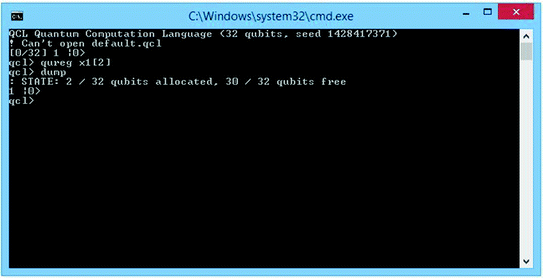
Interface QCL
-
2.
One Particle. Java-applet simulating quantum mechanics, which describes the behavior of a single particle in bound states in one dimension. It solves the Schrödinger equation and allows visualization solutions.
-
3.
Shor. If you press one of the keys located in the lower left corner, there will be an emulation of the corresponding quantum algorithm [8]: Shore (Fig. 3), Grover, Simon, Deutsch or the quantum Fourier transform (Fig. 7).
Fig. 7 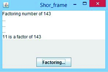
Interface module factorization


The result of the model should be considered:
-
quantum circuits to store it in a separate file and load the parties;
-
color chart model quantum computer;
The result of the quantum register in Fig. 4 can be interpreted and presented in mathematical (complex) with the help of a color table of probabilities/amplitude states of the qubit, which can then be used to study the degree of entanglement of certain pairs qubit model. Displays information about the state of the qubit system using colors provides a more visual data that is easier to take than the numbers, but for the sake of completeness that it is sometimes not enough (Fig. 8).

Decomposition of flowers coloring cells
-
The result of the form to write programs on a quantum programming language QCL;
Naturally, that is QCL can be programmed only very small quantum computing. But this is enough to test the basic algorithms of quantum computing and work them before they will be able to use in full-scale quantum device, which is very useful.
-
Visualization of the behavior of a single particle in bound states in one dimension;
This external unit is able to visualize and simulate the behavior of a single particle in bound states in one dimension and, as a consequence, analyze and predict its future behavior by varying the available parameters. For example, changing the amplitude.
-
The results of calculations of specific quantum algorithms.
The developed model is equipped with a set of specific simulation of quantum algorithms. The article is illustrated by simulation and made a conclusion the results of Shor’s algorithm, the factorization of the number 143 (Fig. 7).
4 Conclusion
The interface of the program is no means the last aspect, which should be given to the development of quantum model of the calculator. It is intuitive and visually intuitive user interface simplifies the process of learning and working. The developed model stands out among its peers convenience, features and clarity. The main advantage of the developed modeling tools to the existing analogues is a modular architecture that allows use of mathematical models of several nuclei. Further studies will improve the GUI environment modeling and the possibility of its setting, as well as increase the functionality through the development of the following areas:
-
Use other libraries, API, for comparative analysis of the performance and capabilities;
-
Increasing the number of operators used;
-
Update the graphics editor of quantum circuits new functionality that extends the current editing quantum circuits;
Analyzed and developed a set of features that will be implemented in a computer and described the core of the interface model and place it in the auxiliary modules and libraries. Was launched a series of third-party modules, the functionality of their graphics (interface) components that run as a result of the model in separate modules, included in its composition.
References
Guzik, V.F., Gushansky, S.M., Potapov, V.S.: The operation algorithm of fundamental elements model of quantum calculator. In: Krukier, L.A., Muratov, G.V., Topolov, V.Y. (eds.) Modern Information Technology: Trends and Prospects: Materials of Conference, pp. 160–162. Southern Federal University Publishing House, South Federal University—Rostov-on-Don (2015)
Guzik, V., Gushanskiy, S., Polenov, M., Potapov, V.: Models of a quantum computer, their characteristics and analysis. In: 2015 9th International Conference on Application of Information and Communication Technologies (AICT), pp. 583–587. Institute of Electrical and Electronics Engineers (2015)
The wave function. https://ru.wikipedia.org/wiki/Wave_function. Accessed 27 Nov 2015
Schrödinger equation. https://ru.wikipedia.org/Schrödinger_equation. Accessed 28 Nov 2015
Guzik, V.F., Gushansky, S.M., Potapov, V.S.: Simulation models of quantum calculator. RF Patent number 2015662926, Russian Patent № 2015619794. Accessed 07 Dec 2015
Guzik, V.F., Gushansky, S.M., Polenov, M.Yu., Potapov, V.S.: Implementation of the components for the construction of an open modular models of quantum computing devices. Informatization Commun. 1, 44–48 (2015)
Guzik, V.F., Gushansky, S.M., Potapov, V.S.: The model of quantum computing. Education and science: the current state and prospects of development. In: Collection of Articles of the International Scientific and Practical Conference, pp. 761–765. Tambov. Accessed 29 Sept 2015
Guzik, V.F., Gushansky, S.M., Potapov, V.S.: Difficulty rating quantum algorithms. Technology of development of information systems. In: Collection of Articles of the International Scientific and Practical Conference, pp. 81–85. Gelendzhik. Accessed 01 Sept 2014
Acknowledgments
This work was supported by RFBR, grant number 15-01-01270 NC\15.
Author information
Authors and Affiliations
Corresponding author
Editor information
Editors and Affiliations
Rights and permissions
Copyright information
© 2016 Springer International Publishing Switzerland
About this paper
Cite this paper
Potapov, V., Gushansky, S., Guzik, V., Polenov, M. (2016). Architecture and Software Implementation of a Quantum Computer Model. In: Silhavy, R., Senkerik, R., Oplatkova, Z.K., Silhavy, P., Prokopova, Z. (eds) Software Engineering Perspectives and Application in Intelligent Systems. ICTIS CSOC 2017 2016. Advances in Intelligent Systems and Computing, vol 465. Springer, Cham. https://doi.org/10.1007/978-3-319-33622-0_6
Download citation
DOI: https://doi.org/10.1007/978-3-319-33622-0_6
Published:
Publisher Name: Springer, Cham
Print ISBN: 978-3-319-33620-6
Online ISBN: 978-3-319-33622-0
eBook Packages: EngineeringEngineering (R0)