Mean–Field Approximation. Quantum Vlasov Equation. Collective Effects

Bonitz, Michael

doi:10.1007/978-3-319-24121-0_4

Mean–Field Approximation. Quantum Vlasov Equation. Collective Effects

Michael Bonitz²

Chapter
First Online: 18 November 2015

2363 Accesses

Abstract

This chapter discusses the simplest many-body approximation—the mean field approximation which amounts to the complete neglect of correlations. Alternative names are Vlasov approximation (in the classical limit) or time-dependent Hartree (or Hartree-Fock), in the quantum literature. Performing a linearization with respect to the perturbing field we derive linear response quantities such as the longitudinal polarization and the dielectric function $\epsilon (\mathbf{k},\omega )$. In the following, collective plasma oscillations and instabilities are discussed for 1D, 2D and 3D quantum systems. The chapter concludes with extensions beyond the linear regime, in particular with the formulation of a quasi-linear theory for quantum systems.

This is a preview of subscription content, log in via an institution.

Chapter: USD 29.95; Price excludes VAT (USA)

eBook: USD 119.00; Price excludes VAT (USA)

Softcover Book: USD 159.99; Price excludes VAT (USA)

Hardcover Book: USD 159.99; Price excludes VAT (USA)

Tax calculation will be finalised at checkout

Purchases are for personal use only

Learn about institutional subscriptions

Notes

1.
In the latter case, this approximation is usually called TDHF (time-dependent Hartree-Fock approximation). For examples of its application to nuclear systems see [145] and references therein.
2.
The more general case, where $U^\mathrm{eff}$ contains also the influence of transverse (electromagnetic) fields, will be discussed in Chaps. 12 and 13.
3.
Much slower than the disturbing potential U(t).
4.
The infinitesimal positive imaginary part of the complex frequency assures the existence of the Laplace transform (4.10). The case of negative imaginary parts is more difficult and requires analytical continuation of $\Pi ^R$ what will be discussed below.
5.
We underline that the above long wavelength limit is not uniquely defined if we take the vector character of $\vec {k}$ serious. The result will depend on the path in momentum space (except for one-dimensional systems or isotropic 2D or 3D systems). Another way to look at this problem is to introduce the Cartesian components of $\vec {k}$ and $\vec {v}$, $(\alpha , \beta )=x,y,z$, which leads to a tensor expression for the polarization
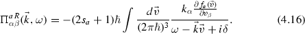
The previous result (4.15) is just the trace of this tensor, i.e. $\Pi ^R_a=\Pi ^{aR}_{xx}+\Pi ^{aR}_{yy}+\Pi ^{aR}_{zz}$.
Of course, the full quantum expression (4.14) has the same tensor structure. We will return to this question in Sect. 4.2, where we consider the electrodynamic definition of the dielectric function.
6.
There, in fact, the kinetic equation contains on the l.h.s. the single-particle energy E(p), which is due to the effect of the lattice on the electrons, as will be shown in Chap. 12.
7.
$\Pi (k,z)$ has a branch cut along the real axis. With the Plemlj formula we have ($\mathcal{P}$ denotes the principal value, cf. Appendix A)
where the discontinuity at the cut is defined by the spectral function
8.
We mention that this approach which gives rise to (“Landau”) damping of collective excitations in a collisionless theory, was heavily debated in the 1950s. Van Kampen demonstrated that the Vlasov equation has solutions (“Van Kampen modes”) which are not damped [152, 153], giving rise e.g. to the Bernstein waves [154]. Later it was shown that both concepts agree if the superposition of all modes is considered [155].
9.
Inserting (4.31, 4.32) into (4.29), we can write down the result for the retarded RPA polarization function on the whole complex frequency plane
$$\begin{aligned} \frac{ \tilde{\Pi }^R(\vec {k},\omega ,\gamma )}{2s+1}=&\left\{ \begin{array}{lcr} \displaystyle {\int \frac{d \vec {p}}{(2\pi \hbar )^3} \frac{ f(E_{\vec {p}}) - f(E_{\vec {p}+\hbar \vec {k}})}{\hbar \omega -i\hbar \gamma -E_{\vec {p}}+E_{\vec {p}+\hbar \vec {k}} } } &{},&{} \gamma <0 \\ \displaystyle { \mathcal{P} \int \frac{d \vec {p}}{(2\pi \hbar )^3} \frac{ f(E_{\vec {p}}) - f(E_{\vec {p}+\hbar \vec {k}})}{\hbar \omega -E_{\vec {p}}+E_{\vec {p}+\hbar \vec {k}} } }\;\;-\nonumber \\ \displaystyle {\frac{i}{2}\int \frac{d\vec {p}}{(2\pi \hbar )^2} \left\{ f(E_{\vec {p}}) - f(E_{\vec {p}}+\hbar \omega ) \right\} } \nonumber \\ \displaystyle { \quad \times \delta [\hbar \omega +E_{\vec {p}}-E_{\vec {p}+\hbar \vec {k}}] } &{},&{} \gamma =0 \\ \displaystyle {\int \frac{d \vec {p}}{(2\pi \hbar )^3} \frac{ f(E_{\vec {p}}) - f(E_{\vec {p}+\hbar \vec {k}})}{\hbar \omega -i\hbar \gamma -E_{\vec {p}}+E_{\vec {p}+\hbar \vec {k}} } } \;\;-\nonumber \\ \displaystyle { i\int _{AC} \frac{d \vec {p}}{(2\pi \hbar )^2} \left\{ f(E_{\vec {p}}) - f(E_{\vec {p}}+\hbar \omega ) \right\} } \nonumber \\ \displaystyle { \quad \times \delta [\hbar \omega +E_{\vec {p}}-E_{\vec {p}+\hbar \vec {k}}] } &{},&{} \gamma >0. \end{array} \right. \end{aligned}$$
In the last line the symbol “AC” denotes that after integration with $\omega $ being real, the result has to be analytically continued into the lower frequency half plane. Usually, this reduces to the substitution of $\omega \rightarrow \omega -i\gamma $ in the argument of the distribution functions. We mention that the complex frequency leads to a complex (momentum) argument in the distribution function. This sometimes gives rise to oscillations in the dielectric function vs. Im $\,\omega $, in particular, if f contains exponentials, as is the case in equilibrium (Maxwell or Fermi/Bose distributions), see for example Fig. 4.2a.
10.
Depending on the system symmetry and the application of external electric or magnetic fields, the solution of (4.41) can be very complicated. In special cases, simplifications are possible. These include
1. (i)
  Dispersion of longitudinal oscillations: if there exists a potential $\phi $ with $\mathbf{E}(\mathbf{q},\omega )=-i \mathbf{q}\phi (\mathbf{q},\omega )$, the dispersion relation is given by $\displaystyle {\sum _{\alpha \beta }\frac{q_{\alpha }q_{\beta }}{q^2} \epsilon _{\alpha \beta }(\mathbf{q},\omega )=0}$.
2. (ii)
  Isotropic plasmas, see below,
3. (iii)
  Two-dimensional plasmas: the exact dispersion relation reads $\displaystyle {\frac{\omega ^4}{c^4}[\epsilon _{1 1}\epsilon _{2 2}-\epsilon _{1 2}\epsilon _{2 1}] -\frac{\omega ^2}{c^2}q_1 q_2[\epsilon _{1 2}+\epsilon _{2 1}]}-q_1^2 q_2^2=0$
4. (iv)
  One-dimensional plasmas: the dielectric function is a scalar, and (4.41) reduces to $\epsilon (\mathbf{q},\omega ) = 0$.
11.
Alternatively, one can solve (4.42) for complex $\mathbf{q}$ as a function of real $\omega $, which yields the spatial behavior of the modes.
12.
The term in brackets is just $-\epsilon ^{a}$, cf. (4.40).
13.
Here we took into account that, in this case, the hermitean and anti-hermitean part of $\epsilon $ coincide with the real and imaginary part, respectively. This result applies also to longitudinal oscillations in an isotropic plasma (with $\epsilon \rightarrow \epsilon ^l$). In 2D, one has to solve $R_{11}I_{22}+ R_{22}I_{11}-R_{12}I_{21}-R_{21}I_{12}=0$ with the result
and, in 3D, $I_{11}R_{22}R_{33}+\dots - I_{33}R_{21}R_{12}=0$, with the solution
where $``\, '\, $” denotes the derivative with respect to $\omega $ at the eigenfrequency $\Omega _s(\mathbf{q})$.
14.
This statement holds also for homogeneous 3D and 2D systems, if their 1D distribution (integrated over the transverse directions) has only one maximum.
15.
Basically, the wavenumber must “fit” in the minimum in order for the wave to gain energy from the particles. We will explicitly confirm this for one-dimensional plasmas below. Interestingly, it turns out that this is not an artifact of the linear approximation. This sensitivity to the wave number is confirmed also in solutions of the full nonlinear kinetic equation, cf. Sect. 4.6.
16.
This is an exceptionally broad field where much work has been done, both experimentally and theoretically. For illustration purposes, we limit ourselves to simple examples of longitudinal plasma oscillations in isotropic systems. For the discussion of transverse (electromagnetic) modes, surface plasmons, interband excitations or magnetic field effects, we will refer to the more specialized literature.
17.
In contrast to 3D systems, where the Coulomb potential is $V(q)=4\pi e^2/(\epsilon _b q^2)$, in a quantum confined system (e.g. quantum wire), V(q) is better approximated by $V(q)=\displaystyle {2\,e^2 K_0(qd)/\epsilon _b}$, where $K_0$ is the modified Bessel function, and $\epsilon _b$ and d are the background dielectric constant and the wire diameter, respectively.
18.
For the analytic continuation of the step function, we use the continuous representation
For complex k, the arctan is a complex function, but the imaginary part vanishes if $\Delta $ goes to zero, and we can drop it.
19.
The $ \Delta \rightarrow 0$ terms arise from the residua of the polarization function’s denominator (4.60). This guarantees that $\mathrm{Im}\Pi $ will be continuous when it crosses the real frequency axis (notice $F_{-\alpha } = - F_{\alpha }$).
20.
These lines include, for example, the $\omega =0$ divergencies at $q=0$ and $q=2k_F$, which are related to the Peierls instability [188].
21.
This mode follows the upper edge of the pair continuum $\Omega _{ac}(q)\approx \omega _1(q)$ and is always strongly damped. Notice also that there exists an undamping region (where $\mathrm{Im}\Pi =0$) which is enclosed by the line $\omega _-(q)$ and the momentum axis [189]. This is a peculiarity of 1D systems, which occurs in 2D or 3D only in non-equilibrium.
22.
Since the mode is undamped, one has to solve only $\mathrm{Re}\,\epsilon =0$ at $\gamma =0$, and we recover from (4.62), (4.63) the result of [189]
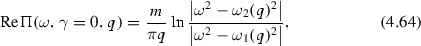
and the imaginary part is $\mathrm{Im}\, \Pi (\omega ,\gamma =0,q)= \frac{m}{\pi q}$ for $\omega _- \le \omega \le \omega _1$ and zero otherwise. The solution of $\mathrm{Re}\,\epsilon (\omega ,\gamma =0,q) = 1-V(q) \mathrm{Re}\,\Pi (\omega ,\gamma =0,q)=0$ is [191]
The long-wavelength ($q\rightarrow 0$) limit for the real part of the polarization is $\mathrm{Re} \Pi (\omega ,\gamma =0,q)= \frac{2 k_F}{\pi m} \frac{q^2}{\omega ^2}+O(q^4)$, where the Fermi momentum is connected with the 1D density via $k_F=n\pi /2$. Taking into account $\lim _{q\rightarrow 0}K_0(qd) \approx - \mathrm{ln}(qd)$, (4.65), gives (4.66).
23.
Formulas of this type are most easily derived from the classical limit of the inverse dielectric function, i.e. the Vlasov dielectric function (4.15). They can be improved phenomenologically to reproduce also the pair continuum. Furthermore, these formulas are straightforwardly generalized to multi-component systems.
24.
The reason for the more complicated shape of the curves $\mathrm{Im}\,\epsilon =0$ and $\mathrm{Re}\,\epsilon =0$ and their additional crossing points is the complicated pole structure of the analytic continuation of the Fermi function . These poles are located at the Matsubara frequencies and give rise to a periodic fractal-like pattern. Only the “original” points carry physical information, and their replicas should be excluded from the plasmon analysis. We mention that this question has been extensively discussed for classical (Maxwell) plasmas, e.g. [193–195].
25.
The same effect occurs in 2D and 3D. For example, for small q, one finds for the frequency of the optical plasmon $\Omega ^{2}(q)\approx \omega _{p}^{2}[1+\alpha (q,n,T)]$, with $\alpha ^{3D}=q^{2}r_{3D}^{2}$ and $\alpha ^{2D}=qr_{2D}$, e.g. [196].
26.
The following model distribution was used, $f_\mathrm{NEQ}(k)=\Theta (k_F-k)\Theta (k)+\Theta (k_4-k)\Theta (k-k_3),\; k_F < k_3 < k_4; k\ge 0; k_F=1.9/a_B, k_3=1.84 k_F, k_4=k_3+k_F$.
27.
Due to (4.21), it is sufficient to prove that $\mathrm{Im}\,\Pi _{a}(\omega ,\gamma ,q)<0$ for any plasma component. The complex polarization function for isotropic 3D systems can be evaluated by introducing spherical coordinates. Defining $z=cos\theta , y=k\,z, u=\frac{m_{a}}{q}\omega \;(\omega \ge 0)$ and $\delta =\frac{m_{a}}{q}\gamma $, one angle integration can be carried out
$$\begin{aligned} \frac{\Pi _a(\omega ,\gamma ,q)}{(2\,s_{a}+1)}=\frac{m_{a}}{q} \int _{0}^{\infty } \frac{dk}{(2 \pi )^{2}}k\,f_{a}(k) \int _{-k}^{k} dy \left\{ \frac{1}{y-\frac{q}{2}-(u-i\delta )}- \frac{1}{y+\frac{q}{2}-(u-i\delta )} \right\} . \nonumber \end{aligned}$$
The imaginary part is easily separated:
$$\begin{aligned} \mathrm{Im}\,\Pi _a(\omega ,\gamma ,q) = - (2\,s_{a}+1)\frac{m_{a}}{q} \int _{0}^{\infty } \frac{dk}{(2 \pi )^{2}}k\,f_{a}(k) \big \{A_{+}-A_{-}\big \}, \nonumber \\ \nonumber \text{ with }\quad A_{\pm }=\arctan \frac{k-(\pm u-\frac{q}{2})}{|\delta |}- \arctan \frac{k-(\pm u+\frac{q}{2})}{|\delta |}. \end{aligned}$$
It is readily verified that $A_{+}-A_{-} \sim \text{ sign }(k)$, so it does not change its sign for non-negative k, and, therefore $\mathrm{Im}\,\Pi _{a}\le 0$.
28.
Of course, in reality, the distribution is never strictly isotropic, already due to fluctuations.
29.
The average can be over a time much larger than the relevant oscillation period, or it can be an average over the spectrum of field fluctuations (plasma turbulence).
30.
Due to the averaging procedure the original reversible Vlasov equation transformed into an irreversible which describes the evolution toward a stationary nonequilibrium state which is accompanied by an entropy increase [225].
31.
More precisely, it has a plateau along the direction of the excited wavenumber.
32.
In contrast to the classical quasilinear equations, the system of equations for the harmonics is reversible and does not lead to a stationary state.
33.
This chapter (as all sections marked with “*”) may be skipped on first reading.
34.
A selfconsistent approach which treats particles and electromagnetic fields (including transverse fields and plasmons) fully selfconsistently, is possible only within quantum electrodynamics and will be considered in Chap. 13.
35.
Of course, strictly speaking, such a subdivision is not possible. There is no unique prescription for it. Moreover, short-range and long-range interactions do overlap and influence each other. However, in the case of dilute systems, where short-range collisions are very rare, this approach may be expected to allow for a qualitative analysis.
36.
For the connection of $b^{\dag }_\mathbf{q}$ and $b_\mathbf{q}$ with the field variables and subsidiary conditions on the latter which guarantee that Maxwell’s equations (12.2) are satisfied, cf. [231].
37.
Of course, there are several problems: The critical momentum $k_c$ is not defined selfconsistently. For quantum plasmas, it is of the order of $k_c \sim \omega _{p}/v_F$, and for classical plasmas of the order of the inverse Debye radius, $k_c \sim k_D=\omega _{p}/(kT/m)^{1/2}$ [126]. Furthermore, the plasmon dispersion $\Omega (q)$ which enters the Hamiltonian, is difficult to calculate selfconsistently too.
38.
The electron equation has the form
$$\begin{aligned}&\frac{\partial f(\mathbf{k})}{\partial t} = \frac{\pi }{\mathcal{V}} \sum _{q<q_c} V_q \Omega (\mathbf{q})\Big \{ \nonumber \\&N_q \; \left\{ [ f(\mathbf{k+q})-f(\mathbf{k}) ] \; \delta \left( \hbar \Omega (\mathbf{q}) - E_\mathbf{k,q} \right) + [ f(\mathbf{k-q})-f(\mathbf{k}) ] \; \delta \left( \hbar \Omega (\mathbf{q}) - E_\mathbf{k,-q} \right) \right\} \nonumber \\+ & {} \left\{ f(\mathbf{k+q})\;[1-f(\mathbf{k}) ] \; \delta \left( \hbar \Omega (\mathbf{q}) - E_\mathbf{k,q} \right) + f(\mathbf{k})\;[1-f(\mathbf{k-q}) ] \; \delta \left( \hbar \Omega (\mathbf{q}) - E_\mathbf{k,-q} \right) \right\} \Big \}. \nonumber \end{aligned}$$
The terms proportional to $N_q$ are gain and loss of electrons, stimulated by resonant absorption of a plasmon with wavenumber $\mathbf{q}$ or $\mathbf{-q}$. In equilibrium, the first contribution is negative, whereas the second is always positive. The terms in the last line describe again spontaneous Cherenkov radiation of electrons which scatter into the corresponding states with lower momentum. Via to the Pauli principle, the scattering rates depend on the population of the final state.

Author information

Authors and Affiliations

Institut für Theoretische Physik, Universität Kiel, Kiel, Germany
Michael Bonitz

Authors

Michael Bonitz
View author publications
You can also search for this author in PubMed Google Scholar

Corresponding author

Correspondence to Michael Bonitz .

Rights and permissions

Reprints and permissions

Copyright information

About this chapter

Cite this chapter

Bonitz, M. (2016). Mean–Field Approximation. Quantum Vlasov Equation. Collective Effects. In: Quantum Kinetic Theory. Springer, Cham. https://doi.org/10.1007/978-3-319-24121-0_4

Download citation

DOI: https://doi.org/10.1007/978-3-319-24121-0_4
Published: 18 November 2015
Publisher Name: Springer, Cham
Print ISBN: 978-3-319-24119-7
Online ISBN: 978-3-319-24121-0
eBook Packages: Physics and AstronomyPhysics and Astronomy (R0)

Publish with us

Policies and ethics