
Abstract
After discussing in detail the method of reduced density operators before, this chapter covers the second approach to correlated quantum many-particle systems out of equilibrium: nonequilibrium Green functions (NEGF). The starting point is the formulation of second quantization which is introduced for fermions coupled to photons within a fully relativistic framework and the definition of particle and photon Green functions, following the work of Schwinger [94, 95]. Nonequilibrium effects are introduced via the Schwinger-Keldysh time contour, and we then derive the key equations: the coupled Keldysh-Kadanoff-Baym equations (KBE) for fermions and photons. Correlation effects are included in full generality, and approximations are formulated in terms of particle and photon selfenergies. After discussing important approximations for the selfenergy, using the concept of the vertex function, we proceed to the dynamics of non-relativistic fermions, decoupling the dynamics from that of the transverse photons. This is followed by an analysis of key properties of the KBE and numerical solutions. A key result is the conservation of total energy and the relaxation towards a correlated (nonideal) equilibrium distribution. In the following more advanced numerical results are presented, including optically excited semiconductors, electrons in quantum dots and plasmas. After treating ultrafast relaxation properties we demonstrate that the nonequilibrium dynamics can also be used to compute high quality equilibrium properties such as susceptibilities, the dynamical structure factor or electronic double excitations in atoms an molecules. Finally, in Sect. 13.9 we establish the connection to the first part of the book—the method of reduced density operators. This is achieved by applying the generalized Kadanoff-Baym ansatz (GKBA) to the KBE—the same ansatz that was independently obtained already in Chaps. 7, 9 and 10. The chapter concludes with results for the ultrafast build up of dynamical screening that is obtained using selfenergies in RPA (GW), by solving for the dynamically screened Coulomb potential \(V_s(t,t')=V_C\varepsilon ^{-1}(t,t')\), as discussed before in Chap. 10. This build up of screening during a finite time resolves the problem of unphysical fast relaxation noted in Chap. 1 and has been nicely confirmed by experiments of Leitenstorfer et al. [69].
Access this chapter
Tax calculation will be finalised at checkout
Purchases are for personal use only
Notes
- 1.
This chapter (as all sections marked with “*”) may be skipped on first reading.
- 2.
For completeness, we mention impressive early work on relativistic kinetic theory by Belyaev and Budker [356], Klimontovich [357, 358] and Silin [359].
- 3.
- 4.
Note that this is not a trivial result. To derive the equations of motion for these operators one has to start from their Heisenberg representation. In second quantization evaluation of the commutator with the Hamiltonian finally leads to these equations.
- 5.
See our discussion in Sect. 2.1.
- 6.
- 7.
The derivation is straightforward but lengthy and can be found e.g. in [45].
- 8.
Here, we follow Dubois’ notation, however, also other definitions appear in the literature. Also, we will use capitals for the quantities on the contour and small letters for the physical quantities.
- 9.
The singular part is missing in many cases.
- 10.
The classical analogue appears in Klimontovich’s phase space density technique [83], where he also considers correlations of particle and field fluctuations \(\, \langle \delta N \delta N \rangle \,\), \(\, \langle \delta E \delta E\rangle \,\) and cross correlations \(\, \langle \delta N \delta E\rangle \,\), for which he derives equations of motion, e.g. [72], see also Sect. 1.5.
- 11.
An exception are “anomalous” situations, such as superconductivity or Bose condensation.
- 12.
We emphasize that only for isotropic media a separation of longitudinal and transverse components is possible. Only in that case, with the use of the Coulomb gauge, the (00) component contains the longitudinal part, while the (ij) components (\(i,j = 1,2,3\)) corresponds to the transverse part, cf. Table 13.1.
- 13.
This is especially transparent in the nonrelativistic limit, see Sect. 13.6.
- 14.
Expression (13.27) follows immediately from the definition of \(\Sigma \), (13.19). To obtain (13.26) from the definition (13.15), one first has to express the current variation \(\delta j^{\mu }\) in terms of \(\delta G\) using (13.3). Finally, \(\delta G\) is expressed via \(\delta G^{-1}\) by means of the identity (G.27), which again gives rise to the initial correlation contribution \(C_{\nu }\).
- 15.
In (13.29), the first term comes from the differentiation of \(G_0^{-1}\), whereas the second comes from applying the chain rule to \(\delta \Sigma /\delta A \sim \delta \Sigma /\delta G\,\cdot \,\delta G/\delta A\). Finally, the variation of G is transformed into a variation of \(G^{-1}\) according to (G.27).
- 16.
It should be pointed out, however, that full selfconsistency creates problems as well. This concerns, in particular, the quality of the photon or plasmon spectrum. An example are possible violations of sum rules, e.g. [362] and references therein.
- 17.
The corresponding relations for a product of two Keldysh matrices are sometimes called Langreth rules, e.g. [10, 11]. Some examples will be given below.
- 18.
The retarded and advanced Green functions and selfenergies then follow from the two correlation functions via (13.10), without the singular term.
- 19.
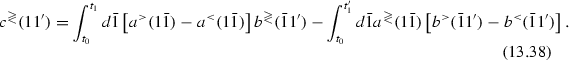
We briefly outline the derivation of (13.36). The “\(>\)” component of an integral over the product or two Keldysh matrices A and B, \(C({\underline{1}},{\underline{1}}')= \int d{\bar{\underline{1}}}A({\underline{1}},{\bar{\underline{1}}})B({\bar{\underline{1}}},{\underline{1}}')\) follows from elementary matrix multiplication, using the notation (13.9) and the Langreth rules [11],

Finally, (13.10) allows to eliminate the “\(\pm \)” functions and also specifies the limits of the time integration, leading to the result which is easily generalized to the \(c^{<}\) component,
In particular, on the time diagonal we have

- 20.
The rules are the following [93]: (1) For each particle-field vertex (thick dot), a factor \(\sqrt{-e^2/\hbar c} \gamma _{\mu }\) is assigned, for each photon line a factor \(4\pi \hbar \eta _{\nu }D^{\mu \nu }\) and for each particle line of species “s” a factor \(\hbar G_s\) (or \(\hbar G_{0s}\)). (2) Over all internal indices (numbers) integration over space and time and summation over the Keldysh branches is implied. (3) For each closed Fermion loop a factor \(-1\) arises. Readers interested in details are referred to [364].
- 21.
In the nonrelativistic limit, the two types of expansions have been compared e.g. in [45].
- 22.
If the system is correlated initially, the g’s are needed also for other time arguments.
- 23.
This is analogous, to Bogolyubov’s functional hypothesis (see Chap. 5).
- 24.
We outline the main steps: First, we recall that the 4-spinor \({\hat{\Psi }}_s\) is composed of two bi-spinors \(({\hat{\psi }}_s,{\hat{\zeta }}_s)\), which may be chosen in a way that \(\zeta _s/\psi _s \sim v/c\). Then, (13.48) is equivalent to the system


If the kinetic and potential energy of the particles are small compared to their rest energy, the first two terms on the l.h.s. of (13.51) may be neglected, and the equation can be solved for \(\zeta \). Inserting the result into (13.50), yields, after some algebra (which can be found e.g. in [343]), the Pauli equation (13.52).
- 25.
This is one possible definition of the field operators. On the other hand, these (anti-)commutation rules are derived straightforwardly from the spinor representation of the field based on the requirement for the total energy to be positive defined, e.g. [343].
- 26.
In the 3-vector notation, there is no distinction between upper and lower indices necessary, so we will use subscripts. Still summation over repeated indices is implied.
- 27.
Compare the discussion in Sect. 4.2.
- 28.
The Coulomb potential in the plasmon Green function arises from the functional differentiation of \(\rho ^{ext}\) in the Maxwell equation for the static potential, i.e. the “0” component of the 4-vector equation (13.1) in Coulomb gauge, \(\Delta \phi =-4\pi (\rho +\rho ^{ext})\).
- 29.
Here and below, \(\sigma \) denotes, as usually, the selfenergy beyond Hartree-Fock.
- 30.
We mention that the introduction of initial correlations in the Kadanoff-Baym equations is essentially more complicated than in the density operator technique (cf. Chap. 6), due to the two-time structure of the former. This question has been discussed by many authors before, e.g. [361, 372, 373], see also the text books [63, 75]. Apparently, the most satisfactory treatment is due to Danielewicz [361], who gives two formulations. One is based on the deformation of the Keldysh contour to imaginary times, but this is applicable only to ground state or equilibrium initial conditions. His second derivation is more general and uses a generalization of Wick’s theorem, and the result agrees with ours. An important requirement noted by Danielewicz is that the initial correlation terms must, on the time diagonal, coincide with the respective density operator expressions.
- 31.
We also mention recent work by Stefanucci and van Leeuwen [375].
- 32.
Notice that the equations for \(V_s^{\pm }\) and \(\pi \) fully agree with our density operator result which was derived in Chap. 10.
- 33.
These equations have been derived in Chap. 9 using the density operator formalism.
- 34.
Notice the similarity of this condition with the conservation criterion for the density operators, Sect. 2.2.2.
- 35.
The natural question of how these two concepts are related will be discussed in Sect. 13.9, in the frame of the Generalized Kadanoff-Baym ansatz (GKBA).
- 36.
First numerical solutions were reported in nuclear matter by Danielewicz [376] which were truly amazing for that time. A decade later more solutions in nuclear matter were performed by Greiner et al. [377] and Köhler, e.g. [378]. First semiconductor applications are due to Schäfer [379], see below.
- 37.
Such a setup is also called “interaction quench” and has now become quite popular in the field ultracold gases.
- 38.
Molecular Dynamics simulations indicate that, for strongly coupled systems, the relaxation may even be oscillatory, see e.g. [296]. This has not been observed in Kadanoff-Baym calculations of macroscopic systems, due to the strong selfconsistent damping (selfenergy).
- 39.
In the case of multicomponent systems the Bloch matrix is simply diagonal in the “band” indices.
- 40.
To simplify the presentation, we will not write the spin argument explicitly restricting ourselves to situations where the populations of spin up and spin down electrons are equal and the external excitation is not spin-sensitive.
- 41.
In the simulations below, we use the rotating wave approximation separating the fast oscillations with the laser carrier frequency, e.g. [196].
- 42.
Note that the oscillations of position and velocity occur with frequency \(\Omega \), whereas kinetic and potential energy (oscillations of \(p^2\) and \(r^2\) have the frequency \(2\,\Omega \)).
- 43.
- 44.
An example is the so-called FROG (frequency resolved optical gating) method developed in [392], for an application to semiconductors, see e.g. [393].
- 45.
Recall that products of Keldysh functions are short notations and are understood as containing a time integral and summation over basis indices, \(AB \rightarrow (AB)_{ij}(t,t') = \sum _k\int _\mathcal{C}d{\bar{t}} A_{ik}(t, {\bar{t}})B_{kj}({\bar{t}},t')\).
- 46.
Note that our linear response derivation recovered this equation without assuming an equilibrium state. Therefore, this result is valid for arbitrary nonequilibrium situations; then all functions are functions on the contour \(\mathcal C\).
- 47.
Intraband transitions were excluded by the form of the dipole matrix element \(d_{\mu \nu } \sim (1-\delta _{\mu \nu })\).
- 48.
The second order function, \(G^{(2)}\), would correspond to the second harmonic with wavenumber 2q.
- 49.
It follows by subtracting the equations for \(g^{>}\) and \(g^{<}\).
- 50.
We do not observe oscillations of \(V^{<}_s\) which is, again, due to the strong selfconsistent damping. Earlier observations [299] were based on calculations with the free (undamped) GKBA.


Author information
Authors and Affiliations
Corresponding author
Rights and permissions
Copyright information
© 2016 Springer International Publishing Switzerland
About this chapter
Cite this chapter
Bonitz, M. (2016). \(*\)Nonequilibrium Green Functions Approach to Field-Matter Dynamics. In: Quantum Kinetic Theory. Springer, Cham. https://doi.org/10.1007/978-3-319-24121-0_13
Download citation
DOI: https://doi.org/10.1007/978-3-319-24121-0_13
Published:
Publisher Name: Springer, Cham
Print ISBN: 978-3-319-24119-7
Online ISBN: 978-3-319-24121-0
eBook Packages: Physics and AstronomyPhysics and Astronomy (R0)