Fields in Interaction

D’Auria, Riccardo; Trigiante, Mario

doi:10.1007/978-3-319-22014-7_12

Riccardo D’Auria¹⁰ &
Mario Trigiante¹⁰

Part of the book series: UNITEXT for Physics ((UNITEXTPH))

3710 Accesses

Abstract

So far we have restricted our analysis to free bosonic and fermionic fields. In this case we were able to canonically quantize them, by associating with the fields and their conjugate momenta operators acting on a Hilbert space of states and satisfying the canonical commutation (or anti-commutation) relations and the equations of motion. This was possible since free fields can be represented as collections of infinitely many decoupled harmonic oscillators, each associated with a given one-particle state.

This is a preview of subscription content, log in via an institution to check access.

Access this chapter

Log in via an institution

Chapter: USD 29.95; Price excludes VAT (USA)

eBook: USD 49.99; Price excludes VAT (USA)

Softcover Book: USD 64.99; Price excludes VAT (USA)

Hardcover Book: USD 89.99; Price excludes VAT (USA)

Tax calculation will be finalised at checkout

Purchases are for personal use only

Institutional subscriptions

Notes

1.
For fermionic fields it is more appropriate to talk about anti-oscillators, being them quantized using anti-commutators in order to reproduce the right statistics.
2.
In this book we often denote states by $\vert \psi \rangle $. The reader should, however, bear in mind that the Greek letter $\psi $ in this symbol has no relation to fermion fields, generically denoted by $\psi (x)$.
3.
This would not be true if, during the interaction process, bound states of particles are formed. The final system at $t\rightarrow +\infty $ would not consist in this case of free-particles only. We shall not consider interactions which allow the creation of bound states.
4.
Here we denote by dV a volume which is infinitesimal but still macroscopic in size, so as to contain a considerable number of particles.
5.
The normalization volumes $V_i$, here and in the following, should be thought of as having a microscopic size, given by the width of the wave packet describing the particle. It should not be confused with the macroscopic volume element dV in which the decay events occur.
6.
Strictly speaking, identifying the fields of the particles long before the interaction process as free is not correct: As we shall see when discussing quantum electrodynamics, although not interacting with each other, charged particles interact with their own electromagnetic field. The effect of this self-interaction will be discussed and taken into account in Sects. 12.7 and 12.8.
7.
Note that, for the sake of notational simplicity, we have simply denoted by $\hat{H}_0$ the free Hamiltonian in the Schroedinger representation as well as in the interaction picture.
8.
The final relations we are going to derive apply to the photon field as well.
9.
In Sects. 12.2.1 and 12.2.2, in contrast to the present section, we were considering collections of particles decaying or interacting (i.e. colliding beams) and thus the densities $\rho $ were referred to multi-particle systems.
10.
Recall our choice of normalization for the single-particle momentum eigenstates: $\langle \mathbf{p},r\vert \mathbf{p}',r'\rangle =\frac{(2\pi \hbar )^3}{V}\,\delta ^3(\mathbf{p}-\mathbf{p}')\,\delta _{rr'}$.
11.
For fermionic fields, in the same approximation, we would find $j_{i\,\mu }(x)\approx \frac{\bar{p}_{i\,\mu }}{m\,c}\,\overline{\psi }_i(x)\,\psi _i(x)$.
12.
This will be shown in detail when proving Wick’s theorem. Each matrix element $\langle \mathbf{p}\vert \hat{\varPhi }\vert 0\rangle $ contains a factor $\sqrt{V}$ coming from the expansion of $\hat{\varPhi }$ in terms of creation and annihilation operators ($a^\dagger ,\,a$, respectively), and a factor $\frac{1}{V}$ coming from the vacuum expectation value (v.e.v.) $\langle 0\vert aa^\dagger \vert 0\rangle $, which equals $\langle 0\vert [a,\,a^\dagger ]\vert 0\rangle =[a,\,a^\dagger ]$ for bosons and $ \{a,\,a^\dagger \}$ for fermions. The matrix element $\langle \mathbf{p}\vert \hat{\varPhi }\vert 0\rangle $ will thus contribute a factor $\frac{1}{\sqrt{V}}$.
13.
We have supposed the dynamics of the process not to depend on the azimuthal angle $\varphi $, which is reasonable for an isolated system of interacting particles: In the case of a head-on collision both $\theta $ and $\varphi $ are referred to the common direction of the two incident particles in the CM frame.
14.
For an elastic collision between two particles of rest masses $m_1,\,m_1$, we have $\mu _1=m_1$, $\mu _2=m_2$ and $|\mathbf{p}|=|\mathbf{q}|$. Using Eq. (12.94) one can easily show that the factor $\sqrt{(p_1\cdot p_2)^2-m_1^2m_2^2\,c^4}$ in the formula (12.81) for the cross-section can be alternatively be written as $\sqrt{s}|\mathbf{p}|=E\,|\mathbf{p}|/c$, $E=E_1+E_2$ being the total energy of the system.
15.
We are familiar with a similar choice for heat and energy: being the mechanical equivalent of heat a universal constant ($4.186\,\mathrm{J/cal}$) we can think of its value as just related to the different operational definitions used for heat and work, so that measuring the two equivalent quantities in the same standard units, namely setting $1\mathrm{cal}=4.186\,\mathrm{J}$, this constant equals one.
By the same token, in the (rationalized) Heaviside-Lorentz system of units, see footnote 1 of Chap. 5, the unit of measurement for the electric charge is defined in terms of the units of length, mass and time by requiring that the vacuum permittivity $\varepsilon _0$ be one.
16.
For the sake of simplicity we shall also denote the commutator and anti-commutator by $[\cdot ,\,\cdot ]_+,\,[\cdot ,\,\cdot ]_-$, respectively. That is: $[\cdot ,\,\cdot ]_+=[\cdot ,\,\cdot ],\,[\cdot ,\,\cdot ]_-=\{\cdot ,\,\cdot \}$.
17.
In order to restore the $\hbar $ and c factors in the covariant derivative, we simply need to replace $e\rightarrow \frac{e}{\hbar \,c}$, as the reader can easily verify.
18.
For the sake of simplicity, we shall suppress the hats on the symbol of the field operators.
19.
Recall that, in the light of our comments below Eq. (12.76), we have replaced everywhere the normalization volume of each particle with 1 / (2E) so that, for instance, $[c(\mathbf{p},r),\,c^\dagger (\mathbf{q},s)]_-=(2\pi )^3\,2E\,\delta _{rs}\,\delta ^{3}(\mathbf{p}-\mathbf{q})$. Note that, had we kept the normalization volumes, the calculation below would yield $\langle 0\vert \psi (x)\vert \mathbf{p},r\rangle =\sqrt{\frac{m}{E_{\mathbf{p}} V}}\,u(\mathbf{p},r)\,e^{-i\,p\cdot x}$, contributing a factor $1/\sqrt{V}$ to the amplitude, as anticipated in our discussion below Eq. (12.76).
20.
The same interpretation is of course also true for the interaction between electron and positron in Bhabha scattering, see Sect. 12.5.3. For the sake of definiteness and simplicity we shall refer the considerations of this subsection to the Möller scattering.
21.
In this special case this can be also seen directly. Indeed
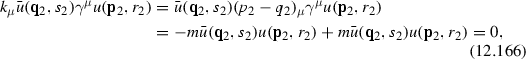
and similarly for the other factor of Eq. (12.167).
22.
In the case of polarized fermions, there would be no summation over the spin states and we should use, for each particle, the expressions in Sect. 10.6.3 for the projector on the corresponding polarization:
$$ u(\mathbf{p},r)\, \bar{u}(\mathbf{p},r)=\frac{(p\!\!/+m)}{4m}\,(\mathbf{1}+\varepsilon _r\gamma ^5n\!\!/),\quad v(\mathbf{p},s)\, \bar{v}(\mathbf{p},s)=\frac{(p\!\!/-m)}{4m}\,(\mathbf{1}-\varepsilon _s\gamma ^5n\!\!/).$$
23.
Note that, in order to restore the $\hbar ,\,c$ factors, we would need to multiply Eq. (12.220) by $\hbar ^2$, while Eq. (12.221) needs no $\hbar ,\,c$ factors to be restored.
24.
The factor $\frac{1}{2}$ is canceled by the sum of the two identical terms (6) an (7) of Eq. (12.140).
25.
Here and in the following we shall omit, for the sake of simplicity, the integration prescription defined by the infinitesimal term $i\epsilon $ in the Feynman propagators.
26.
The expansion is easily derived from the identity
$$ \frac{1}{A+B}=\frac{1}{A}(A+B-B)\frac{1}{A+B}=\frac{1}{A}-\frac{1}{A}B\frac{1}{A+B}. $$
27.
Note that this relation is obtained by gauge-transforming the polarization vectors in (12.244) according to (12.185), and requiring the variation of the amplitude to vanish.
28.
Note that the problem of the electron self-energy already exists in the classical theory of the electron. Indeed, either one assumes the electron to be a point particle without structure, in which case the total energy of the electron together its associated field is infinite; or one assumes a finite electron radius, in which case it should explode as a consequence of the internal charge distribution.
29.
Here and in the following we shall refer, for simplicity, only to electron wave functions u(p, s), to electron lines and so on. However all our analysis equally applies to the electron antiparticle, the positron, as well as to, any other charged lepton, like muons and tau mesons.
30.
There are in principle further divergences associated with the so-called photon-photon system, Fig. 12.13d and the three-photon vertex, Fig. 12.13e. Such divergences are however armless (see below.).
31.
To derive these relations, one can cut each internal fermion line of a diagram into two parts. The total number of lines so obtained should be twice the number of vertices. In this counting however, each internal line contributes two units (i.e. a total of $2F_i$ units) and each external ones a single unit (i.e. a total of $F_e$ units). A similar argument applies to the boson lines.
32.
Actually, beyond 1-loop, there are divergences that require a more careful treatment than just separation into a divergent and a finite part (overlapping divergences). We can neglect them, since we are going to discuss only 1-loop self-energy and vertex insertions which cannot give rise to this kind of divergences.
33.
See Weinberg’s book [13].
34.
Note that if (12.264) were taken between external (on-shell) electron lines, we would recover the electron self-energy computed in Sect. 12.7, namely Eq. (12.241).
35.
Actually we could make the chain approximation (12.264) exact if we would consider each electron self energy insertion not restricted to one-loop order. This can be done by introducing the concept of one particle irreducible (1PI) diagram. A diagram is 1PI if it cannot be disconnected by cutting one internal line. Thus we may consider a self-energy diagram which has contributions from 1PI diagram only, like the three fourth order diagrams of Fig. 12.17a, while the graph (b), being reducible, would not contribute. The reason for selecting only 1PI diagrams is that the reducible diagrams can always be decomposed in 1PI diagrams without further integration, and therefore if we can take care of the divergences of the 1PI diagrams, we automatically take care of the general diagram. Let us denote the correction to the free propagator due to the sum of all possible 1PI self-energy diagrams by $-i\varSigma ^*(p)$, see Fig. 12.18a. The correction (12.264) becomes

If we now perform the chain expansion as in (12.265) but with $-i\varSigma (^p)$ replaced by $-i\varSigma ^*(p)$, we obtain the exact propagator in the form

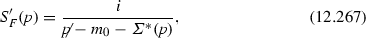
see Fig. 12.18b. In the following however we will limit ourself to consider the approximation (12.264) where only the 1-loop integral $\varSigma (^p)$, lowest order approximation of $\varSigma ^*(p)$, appears.
36.
Naively one could think that the separation of the physical mass into the bare mass $m_0$ and the mass-shift $\delta m =\varSigma (m)$ would correspond to the separation of the electron mass into a “mechanical” and a “electromagnetic” mass. However such separation is devoid of physical meaning since it cannot be observed. We also note that the process of mass renormalization is not a peculiarity of field theory. For example when an electron moves inside a solid it has a renormalized mass $m^*$, also called effective mass, which is different from the mass measured in the absence of the solid, i.e. the bare mass $m_0$. However, differently from our case, the effective and bare mass can be measured separately, while in field theoretical case $m_0$ cannot be measured.
37.
We observe that this term would give a vanishing contribution if we had an external on-shell state instead of the propagator in (12.264) since the term $B(\not \!\!{p}-m)$ in Eq. (12.269) is zero on the free electron wave function.
38.
Recall that a one-particle state and its wave function $\psi (x)$ is related to the quantum fields $\hat{\psi }$ by $\langle 0\vert \hat{\psi }(x) \vert a\rangle $, see for example Eq. (12.64) for a boson particle.
39.
The discussion made in footnote 35 about the exact electron propagator also applies to the photon case. We can express the exact photon propagator as the sum of chains of insertions $\varPi ^{*\mu \nu }(k)$ each representing the sum of all the 1PI diagrams to the photon propagator. We shall restrict, for the sake of simplicity, to the chain approximation of the photon propagator, in which $\varPi ^{*\mu \nu }(k)$ is approximated, to lowest order, by $\varPi ^{\mu \nu }(k)$.
40.
With respect to Eq. (12.163) we have replaced the coupling constant e with $e_0$ since the amplitude was computed to lowest order in the coupling constant.
41.
The seeming singularity due to the presence of the delta function is actually due to our approximation $|\mathbf {k}|^2\ll m^2$. In general the correction will be smooth and strongly peaked around $\mathbf {x}=0$.
42.
To show this use the general on-shell identity (which only holds on-shell):
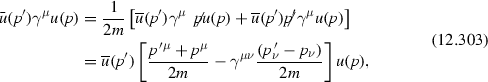
where we have written $ \gamma ^\mu \gamma ^\nu =\eta ^{\mu \nu }+\gamma ^{\mu \nu },$ and $\gamma ^{\mu \nu }$ being defined as $ [\gamma ^\mu ,\gamma ^\nu ]/2$.
43.
See Weinberg’s book [13] for a general derivation of this formula. There the most general form of $\varGamma ^\mu (p',p)$ is written in terms of $\gamma $-matrices, p and $p'$. The number of independent terms reduces considerably upon using the Dirac equation $p\!\!/u(p)=m u(p)$ ($\bar{u}(p')p\!\!/'=m\,\bar{u}(p')$) and the identity (12.303). By further implementing the gauge invariance condition (12.299) the final expression boils down to the one in Eq. (12.306).
44.
Corrections given by the finite parts of loop diagrams are often referred to as radiative corrections.
45.
Since in order to test QED predictions for higher order corrections to a given quantity (like the $g-factor$), a high-precision determination of the coupling constant $\alpha $ is needed, one uses the QED formulas to experimentally determine $\alpha $. QED is then tested by comparing the values of $\alpha $ determined from different experiments.

Author information

Authors and Affiliations

Polytechnic University of Turin, Torino, Italy
Riccardo D’Auria & Mario Trigiante

Authors

Riccardo D’Auria
View author publications
You can also search for this author in PubMed Google Scholar
Mario Trigiante
View author publications
You can also search for this author in PubMed Google Scholar

Corresponding author

Correspondence to Riccardo D’Auria .

Rights and permissions

Reprints and permissions

Copyright information

About this chapter

Cite this chapter

D’Auria, R., Trigiante, M. (2016). Fields in Interaction. In: From Special Relativity to Feynman Diagrams. UNITEXT for Physics. Springer, Cham. https://doi.org/10.1007/978-3-319-22014-7_12

Download citation

DOI: https://doi.org/10.1007/978-3-319-22014-7_12
Published: 07 October 2015
Publisher Name: Springer, Cham
Print ISBN: 978-3-319-22013-0
Online ISBN: 978-3-319-22014-7
eBook Packages: Physics and AstronomyPhysics and Astronomy (R0)

Publish with us

Policies and ethics