
Abstract
We introduce skipping refinement, a new notion of correctness for reasoning about optimized reactive systems. Reasoning about reactive systems using refinement involves defining an abstract, high-level specification system and a concrete, low-level implementation system. One then shows that every behavior allowed by the implementation is also allowed by the specification. Due to the difference in abstraction levels, it is often the case that the implementation requires many steps to match one step of the specification, hence, it is quite useful for refinement to directly account for stuttering. Some optimized implementations, however, can actually take multiple specification steps at once. For example, a memory controller can buffer the commands to the memory and at a later time simultaneously update multiple memory locations, thereby skipping several observable states of the abstract specification, which only updates one memory location at a time. We introduce skipping simulation refinement and provide a sound and complete characterization consisting of “local” proof rules that are amenable to mechanization and automated verification. We present case studies that highlight the applicability of skipping refinement: a JVM-inspired stack machine, a simple memory controller and a scalar to vector compiler transformation. Our experimental results demonstrate that current model-checking and automated theorem proving tools have difficulty automatically analyzing these systems using existing notions of correctness, but they can analyze the systems if we use skipping refinement.
This research was supported in part by DARPA under AFRL Cooperative Agreement No. FA8750-10-2-0233, by NSF grants CCF-1117184 and CCF-1319580, and by OSD under contract FA8750-14-C-0024.
You have full access to this open access chapter, Download conference paper PDF
1 Introduction
Refinement is a powerful method for reasoning about reactive systems. The idea is to prove that every execution of the concrete system being verified is allowed by the abstract system. The concrete system is defined at a lower level of abstraction, so it is usually the case that it requires several steps to match one high-level step of the abstract system. Thus, notions of refinement usually directly account for stuttering [5, 10, 13].
Engineering ingenuity and the drive to build ever more efficient systems has led to highly-optimized concrete systems capable of taking single steps that perform the work of multiple abstract steps. For example, in order to reduce memory latency and effectively utilize memory bandwidth, memory controllers often buffer requests to memory. The pending requests in the buffer are analyzed for address locality and then at some time in the future, multiple locations in the memory are read and updated simultaneously. Similarly, to improve instruction throughput, superscalar processors fetch multiple instructions in a single cycle. These instructions are analyzed for instruction-level parallelism (e.g., the absence of data dependencies) and, where possible, are executed in parallel, leading to multiple instructions being retired in a single cycle. In both these examples, in addition to stuttering, a single step in the implementation may perform the work of multiple abstract steps, e.g., by updating multiple locations in memory and retiring multiple instructions in a single cycle. Thus, notions of refinement that only account for stuttering are not appropriate for reasoning about such optimized systems. In Sect. 3, we introduce skipping refinement, a new notion of correctness for reasoning about reactive systems that “execute faster” and therefore can skip some steps of the specification. Skipping can be thought of as the dual of stuttering: stuttering allows us to “stretch” executions of the specification system and skipping allows us to “squeeze” them.
An appropriate notion of correctness is only part of the story. We also want to leverage the notion of correctness in order to mechanically verify systems. To this end, in Sect. 4, we introduce Well-Founded Skipping, a sound and complete characterization of skipping simulation that allows us to prove refinement theorems about the kind of systems we consider using only local reasoning. This characterization establishes that refinement maps always exist for skipping refinement. In Sect. 5, we illustrate the applicability of skipping refinement by mechanizing the proof of correctness of three systems: a stack machine with an instruction buffer, a simple memory controller, and a simple scalar-to-vector compiler transformation. We show experimentally that by using skipping refinement current model-checkers are able to verify systems that otherwise are beyond their capability to verify. We end with related work and conclusions in Sects. 6 and 7.
Our contributions include (1) the introduction of skipping refinement, which is the first notion of refinement to directly support reasoning about optimized systems that execute faster than their specifications (as far as we know) (2) a sound and complete characterization of skipping refinement that requires only local reasoning, thereby enabling automated verification and showing that refinement maps always exist (3) experimental evidence showing that the use of skipping refinement allows us to extend the complexity of systems that can be automatically verified using state-of-the-art model checking and interactive theorem proving technology.
2 Motivating Examples
To illustrate the notion of skipping simulation, we consider a running example of a discrete-time event simulation (DES) system. A state of the abstract, high-level specification system is a three-tuple \(\langle t, E, A\rangle \) where t is a natural number corresponding to the current time, E is a set of pairs \((e, t_e)\) where e is an event scheduled to be executed at time \(t_e\) (we require that \(t_e \ge t\)), and A is an assignment of values to a set of (global) state variables. The transition relation for the abstract DES system is defined as follows. If there is no event of the form \((e, t) \in E\), then there is nothing to do at time t and so t is incremented by 1. Otherwise, we (nondeterministically) choose and execute an event of the form \((e, t) \in E\). The execution of an event can modify the state variables and can also generate a finite number of new events, with the restriction that the time of any generated event is \(>t\). Finally, execution involves removing (e, t) from E.
Now, consider an optimized, concrete implementation of the abstract DES system. As before, a state is a three-tuple \(\langle t, E, A \rangle \). However, unlike the abstract system which just increments time by 1 when no events are scheduled for the current time, the optimized system uses a priority queue to find the next event to execute. The transition relation is defined as follows. An event \((e, t_e)\) with the minimum time is selected, t is updated to \(t_e\) and the event e is executed, as above.
Notice that the optimized implementation of the discrete-time event simulation system can run faster than the abstract specification system by skipping over abstract states when no events are scheduled for execution at the current time. This is neither a stuttering step nor corresponds to a single step of the specification. Therefore, it is not possible to prove that the implementation refines the specification using notions of refinement that only allow stuttering [13, 17], because that just is not true. But, intuitively, there is a sense in which the optimized DES system does refine the abstract DES system. Skipping refinement is our attempt at formally developing the theory required to rigorously reason about these kinds of systems.
Due to its simplicity, we will use the discrete-time event simulation example in later sections to illustrate various concepts. After the basic theory is developed, we provide an experimental evaluation based on three other motivating examples. The first is a JVM-inspired stack machine that can store instructions in a queue and then process these instructions in bulk at some later point in time. The second example is an optimized memory controller that buffers requests to memory to reduce memory latency and maximize memory bandwidth utilization. The pending requests in the buffer are analyzed for address locality and redundant writes and then at some time in the future, multiple locations in the memory are read and updated in a single step. The final example is a compiler transformation that analyzes programs for superword-level parallelism and, where possible, replaces multiple scalar instructions with a compact SIMD instruction that concurrently operates on multiple words of data. All of these examples require skipping refinement, because the optimized concrete systems can do more than inject stuttering steps in the executions specified by their specification systems; they can also collapse executions.
3 Skipping Simulation and Refinement
In this section, we introduce the notions of skipping simulation and refinement. We do this in the general setting of labeled transition systems where we allow state space sizes and branching factors of arbitrary infinite cardinalities.
We start with some notational conventions. Function application is sometimes denoted by an infix dot “.” and is left-associative. For a binary relation R, we often write xRy instead of \((x, y) \in R\). The composition of relation R with itself i times (for \(0 < i \le \omega \)) is denoted \(R^i\) (\(\omega = {\mathbb {N}}\) and is the first infinite ordinal). Given a relation R and \(1<k\le \omega \), \(R^{<k}\) denotes \(\bigcup _{1 \le i < k} R^i\) and \(R^{\ge k}\) denotes \(\bigcup _{\omega > i \ge k} R^i\) . Instead of \(R^{< \omega }\) we often write the more common \(R^+\). \(\uplus \) denotes the disjoint union operator. Quantified expressions are written as \(\langle Q x :r :p \rangle \), where Q is the quantifier (e.g., \(\exists , \forall \)), x is the bound variable, r is an expression that denotes the range of x (true if omitted), and p is the body of the quantifier.
Definition 1
A labeled transition system (TS) is a structure \(\langle S, \rightarrow ,L\rangle \), where S is a non-empty (possibly infinite) set of states, \(\rightarrow \;\ \subseteq S \times S\) is a left-total transition relation (every state has a successor), and L is a labeling function: its domain is S and it tells us what is observable at a state.
A path is a sequence of states such that for adjacent states s and u, \(s \rightarrow \;u\). A path, \(\sigma \), is a fullpath if it is infinite. \(\textit{fp}.\sigma .s\) denotes that \(\sigma \) is a fullpath starting at s and for \(i \in \omega , \sigma (i)\) denotes the \(i^{th}\) element of path \(\sigma \).
Our definition of skipping simulation is based on the notion of matching, which we define below. Informally, we say a fullpath \(\sigma \) matches a fullpath \(\delta \) under relation B if the fullpaths can be partitioned into non-empty, finite segments such that all elements in a particular segment of \(\sigma \) are related to the first element in the corresponding segment of \(\delta \).
Definition 2
(Match). Let INC be the set of strictly increasing sequences of natural numbers starting at 0. Given a fullpath \(\sigma \), the \(i^{th}\) segment of \(\sigma \) with respect to \(\pi \in INC\), written \(\mathbin {^{\pi }\sigma ^{i}}\), is given by the sequence \(\langle \) \(\sigma (\pi .i),...., \sigma (\pi .(i+1) -1)\rangle \). For \(\pi , \xi \in INC\) and relation B, we define

In Fig. 1, we illustrate our notion of matching using our running example of a discrete-time event simulation system. Let the set of state variables be \(\{v_1,v_2\}\) and let the set of events contain \(\{(e_1, 0), (e_2,2)\}\), where event \(e_i\) increments variable \(v_i\) by 1. In the figure, \(\sigma \) is a fullpath of the concrete system and \(\delta \) is a fullpath of the abstract system. (We only show a prefix of the fullpaths.) The other parameter for \( match \) is B, which, for our example, is just the identity relation. In order to show that \( match(B,\sigma ,\delta ) \) holds, we have to find \(\pi , \xi \) satisfying the definition. In the figure, we separate the partitions induced by our choice for \(\pi , \xi \) using  and connect elements related by B with

. Since all elements of a \(\sigma \) partition are related to the first element of the corresponding \(\delta \) partition, \( corr(B,\sigma ,\pi ,\delta ,\xi ) \) holds, therefore, \( match(B,\sigma ,\delta ) \) holds.

Discrete-time Event simulation system
Given a labeled transition system \(\mathcal {M_{\text {}}}= \langle S_{}, \xrightarrow {}, L_{} \rangle \), a relation \(B \subseteq S \times S\) is a skipping simulation, if for any \(s,w \in S\) such that sBw, s and w are identically labeled and any fullpath starting at s can be matched by some fullpath starting at w.
Definition 3
(Skipping Simulation). \(B \subseteq S \times S\) is a skipping simulation (SKS) on TS \(\mathcal {M_{\text {}}}= \langle S_{}, \xrightarrow {}, L_{} \rangle \) \( iff \) for all s, w such that sBw, the following hold.

It may seem counter-intuitive to define skipping refinement with respect to a single transition system, since our ultimate goal is to relate transition systems at different levels of abstraction. Our current approach has certain technical advantages and we will see how to deal with two transition systems shortly.
In our running example of a discrete-time event simulation system, neither the optimized concrete system nor the abstract system stutter, i.e., they do not require multiple steps to complete the execution of an event. However, suppose that the abstract and concrete system are modified so that execution of an event takes multiple steps. For example, suppose that the execution of \(e_1\) in the concrete system (the first partition of \(\sigma \) in Fig. 1) takes 5 steps and the execution of \(e_1\) in the abstract system (the first partition of \(\delta \) in Fig. 1) takes 3 steps. Now, our abstract system is capable of stuttering and the concrete system is capable of both stuttering and skipping. Skipping simulation allows this, i.e., we can define \(\pi ,\xi \) such that \(corr{B}{\sigma }{\pi }{\delta }{\xi }\) still holds.
Note that skipping simulation differs from weak simulation [10]; the latter allows infinite stuttering. Since we want to distinguish deadlock from stuttering, it is important we distinguish between finite and infinite stuttering. Skipping simulation also differs from stuttering simulation, as the former allows an concrete system to skip steps of the abstract system and therefore run “faster” than the abstract system. In fact, skipping simulation is strictly weaker than stuttering simulation.
3.1 Skipping Refinement
We now show how the notion of skipping simulation, which is defined in terms of a single transition system, can be used to define the notion of skipping refinement, a notion that relates two transition systems: an abstract transition system and a concrete transition system. In order to define skipping refinement, we make use of refinement maps, functions that map states of the concrete system to states of the abstract system. Refinement maps are used to define what is observable at concrete states. If the concrete system is a skipping refinement of the abstract system, then its observable behaviors are also behaviors of the abstract system, modulo skipping (which includes stuttering). For example, in our running example, if the refinement map is the identity function then any behavior of the optimized system is a behavior of the abstract system modulo skipping.
Definition 4
(Skipping Refinement). Let \(\mathcal{M}_{A}=\langle S_{A},{\displaystyle \mathop {\rightarrow }^{A}},L_{A}\rangle \) and \(\mathcal{M}_{C}=\langle S_{C},{\displaystyle \mathop {\rightarrow }^{C}},L_{C}\rangle \) be transition systems and let \({r : S_C \rightarrow S_A}\) be a refinement map. We say \(\mathcal{M}_{C}\) is a skipping refinement of \(\mathcal{M}_{A}\) with respect to r, written \(\mathcal{M}_{C} \lesssim _r \mathcal{M}_{A}\), if there exists a relation \(B \subseteq S_C \times S_A\) such that all of the following hold.
-
1.
\(\langle \forall s \in S_C {:}: sBr.s\rangle \) and
-
2.
B is an SKS on \(\langle S_{C}\uplus S_{A},{\displaystyle \mathop {\rightarrow }^{C}}\uplus {\displaystyle \mathop {\rightarrow }^{A}},\mathcal{L}\) where \(\mathcal{L}.s = L_A(s)\) for \(s \in S_A\), and \(\mathcal{L}.s = L_A(r.s)\) for \(s \in S_C\).
Notice that we place no restrictions on refinement maps. When refinement is used in specific contexts it is often useful to place restrictions on what a refinement map can do, e.g., we may require for every \(s \in S_C\) that \(L_A(r.s)\) is a projection of \(L_C(s)\). Also, the choice of refinement map can have a big impact on verification times [18]. Our purpose is to define a general theory of skipping, hence, we prefer to be as permissive as possible.
4 Automated Reasoning
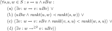
To prove that transition system \(\mathcal {M}_{C}\) is a skipping refinement of transition system \(\mathcal {M}_{A}\), we use Definitions 3 and 4, which require us to show that for any fullpath from \(\mathcal {M}_{C}\) we can find a “matching” fullpath from \(\mathcal {M}_{A}\). However, reasoning about the existence of infinite sequences can be problematic using automated tools. In order to avoid such reasoning, we introduce the notion of well-founded skipping simulation. This notion allows us to reason about skipping refinement by checking mostly local properties, i.e., properties involving states and their successors. The intuition is, for any pair of states s, w, which are related and a state u such that \(s \xrightarrow {} u\), there are four cases to consider (Fig. 2): (a) either we can match the move from s to u right away, i.e., there is a v such that \(w \xrightarrow {} v\) and u is related to v, or (b) there is stuttering on the left, or (c) there is stuttering on the right, or (d) there is skipping on the left.

Well-founded skipping simulation
Definition 5
(Well-founded Skipping). \(B \subseteq S \times S \) is a well-founded skipping relation on TS \(\mathcal {M_{\text {}}}= \langle S_{}, \xrightarrow {}, L_{} \rangle \) iff :
-
(WFSK1) \(\langle \forall s,w \in S :s B w :L.s = L.w\rangle \)
-
(WFSK2) There exist functions, \( rankt :S\times S \rightarrow W\), \( rankl :S \times S \times S \rightarrow \omega \), such that \(\langle W, \prec \rangle \) is well-founded and

In the above definition, notice that condition (2d) requires us to check that there exists a v such that v is reachable from w and uBv holds. Reasoning about reachability is not local in general. However, for the kinds of optimized systems we are interested in, we can reason about reachability using local methods because the number of abstract steps that a concrete step corresponds to is bounded by a constant. As an example, the maximum number of high-level steps that a concrete step of an optimized memory controller can correspond to is the size of the request buffer; this is a constant that is determined early in the design. Another option is to replace condition (2d) with a condition that requires only local reasoning. While this is possible, in light of the above comments, the increased complexity is not justified.
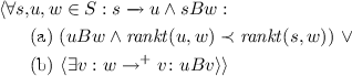
Next, we show that the notion of well-founded skipping simulation is equivalent to SKS and can be used as a sound and complete proof rule to check if a given relation is an SKS. This allows us to match infinite sequences by checking local properties and bounded reachability. To show this we first introduce an alternative definition for well-founded skipping simulation. The motivation for doing this is that the alternate definition is useful for proving the soundness and completeness theorems. It also allows us to highlight the idea behind the conditions in the definition of well-founded skipping simulation. The simplification is based on two observations. First, it turns out that (d) and (a) together subsume (c), so in the definition below, we do not include case (c). Second, if instead of \(\rightarrow ^{\ge 2}\) we use \(\rightarrow ^+\) in (d), then we subsume case (a) as well.
Definition 6
\(B \subseteq S \times S \) is a reduced well-founded skipping relation on TS \(\mathcal {M_{\text {}}}= \langle S_{}, \xrightarrow {}, L_{} \rangle \) iff \(:\)
-
(RWFSK1) \(\langle \forall s,w \in S :s B w :L.s = L.w\rangle \)
-
(RWFSK2) There exists a function, \( rankt :S\times S \rightarrow W\), such that \(\langle W, \prec \rangle \) is well-founded and

In the sequel, “WFSK” is an abbreviation for “well-founded skipping relation” and, similarly, “RWFSK” is an abbreviation for “reduced well-founded skipping relation.”
We now show that WFSK and RWFSK are equivalent.
Theorem 1
B is a WFSK on \(\mathcal {M_{\text {}}}= \langle S_{}, \xrightarrow {}, L_{} \rangle \) iff B is an RWFSK on \(\mathcal {M}\).
Proof
(\(\Leftarrow \) direction): This direction is easy.
(\(\Rightarrow \) direction): The key insight is that WFSK2c is redundant. Let \(s,u, w \in S\), \(s \rightarrow u\), and sBw. If WFSK2a or WFSK2d holds then RWFSK2b holds. If WFSK2b holds, then RWFSK2a holds. So, what remains is to assume that WFSK2c holds and neither of WFSK2a, WFSK2b, or WFSK2d hold. From this we will derive a contradiction.
Let \(\delta \) be a path starting at w, such that only WFSK2c holds between \(s, u, \delta .i\). There are non-empty paths that satisfy this condition, e.g., let \(\delta = \langle w \rangle \). In addition, any such path must be finite. If not, then for any adjacent pair of states in \(\delta \), say \(\delta .k\) and \(\delta (k + 1)\), \( rankl (\delta (k+1),s,u) < rankl (\delta .k,s,u)\), which contradicts the well-foundedness of \( rankl \). We also have that for every \(k>0\), \(u\; B\!\!\!\!/\; \delta .k\); otherwise WFSK2a or WFSK2d holds. Now, let \(\delta \) be a maximal path satisfying the above condition, i.e., every extension of \(\delta \) violates the condition. Let x be the last state in \(\delta \). We know that sBx and only WFSK2c holds between s, u, x, so let y be a witness for WFSK2c, which means that sBy and one of WFSK2a,b, or d holds between s, u, y. WSFK2b can’t hold because then we would have uBy (which would mean WFSK2a holds between s, u, x). So, one of WFSK2a,d has to hold, but that gives us a path from x to some state v such that uBv. The contradiction is that v is also reachable from w, so WFSK2a or WFSK2d held between s, u, w. \(\quad \square \)
Let’s now discuss why we included condition WFSK2c. The systems we are interested in verifying have a bound—determined early early in the design—on the number of skipping steps possible. The problem is that RWSFK2b forces us to deal with stuttering and skipping steps in the same way, while with WFSK any amount of stuttering is dealt with locally. Hence, WFSK should be used for automated proofs and RWFSK can be used for meta reasoning.
One more observation is that the proof of Theorem 1, by showing that WFSK2c is redundant, highlights why skipping refinement subsumes stuttering refinement. Therefore, skipping refinement is a weaker, but more generally applicable notion of refinement than stuttering refinement.
In what follows, we show that the notion of RWFSK (and by Theorem 1 WFSK) is equivalent to SKS and can be used as a sound and complete proof rule to check if a given relation is an SKS. This allows us to match infinite sequences by checking local properties and bounded reachability. We first prove soundness, i.e., any RWFSK is an SKS. The proof proceeds by showing that given a RWFSK relation B, sBw, and any fullpath starting at s, we can recursively construct a fullpath \(\delta \) starting at w, and increasing sequences \(\pi ,\xi \) such that fullpath at s matches \(\delta \).
Theorem 2
(Soundness). If B is an RWFSK on \(\mathcal {M}_{}\) then B is a SKS on \(\mathcal {M}_{}\).
Proof
To show that B is an SKS on \(\mathcal {M_{\text {}}}= \langle S_{}, \xrightarrow {}, L_{} \rangle \), we show that given B is a RWFSK on \(\mathcal {M_{\text {}}}= \langle S_{}, \xrightarrow {}, L_{} \rangle \) and \(x, y \in S\) such that xBy, SKS1 and SKS2 hold. SKS1 follows directly from condition 1 of RWSFK.
Next we show that SKS2 holds. We start by recursively defining \(\delta \). In the process, we also define partitions \(\pi \) and \(\xi \). For the base case, we let \(\pi .0 = 0\), \(\xi .0 = 0\) and \(\delta .0 = y\). By assumption \(\sigma (\pi .0) B \delta (\xi .0)\). For the recursive case, assume that we have defined \(\pi .0, \ldots , \pi .i\) as well as \(\xi .0, \ldots , \xi .i\) and \(\delta .0, \ldots , \delta (\xi .i)\). We also assume that \(\sigma (\pi .i) B \delta (\xi .i)\). Let s be \(\sigma (\pi .i)\); let u be \(\sigma (\pi .i + 1)\); let w be \(\delta (\xi .i)\). We consider two cases.
First, say that RWFSK2b holds. Then, there is a v such that \(w \rightarrow ^{+}{v}\) and uBv. Let \({\displaystyle \mathop {v}^{\rightarrow }} = [v_0 = w, \ldots , v_m = v]\) be a finite path from w to v where \(m \ge 1\). We define \(\pi (i+1) = \pi .i + 1, \xi (i+1) = \xi .i + m\), \( ^\xi \delta ^i = [v_0, \ldots , v_{m-1}]\) and \(\delta (\xi (i + 1)) = v\).
If the first case does not hold, i.e., RWFSK2b does not hold, and RWFSK2a does hold. We define J to be the subset of the positive integers such that for every \(j \in J\), the following holds.
The first thing to observe is that \(1 \in J\) because \(\sigma (\pi .i + 1) = u\), RWFSK2b does not hold (so the first conjunct is true) and RWFSK2a does (so the second conjunct is true). The next thing to observe is that there exists a positive integer \(n>1\) such that \(n \not \in J\). Suppose not, then for all \(n \ge 1, n \in J\). Now, consider the (infinite) suffix of \(\sigma \) starting at \(\pi .i\). For every adjacent pair of states in this suffix, say \(\sigma (\pi .i + k)\) and \(\sigma (\pi .i+k+1)\) where \(k \ge 0\), we have that \(\sigma (\pi .i+k)Bw\) and that only RWFSK2a applies (i.e., RWFSK2b does not apply). This gives us a contradiction because \( rankt \) is well-founded. We can now define n to be \( min (\{l : l \not \in J\})\). Notice that only RWFSK2a holds between \(\sigma (\pi .i + n-1)), \sigma (\pi .i + n)\) and w, hence \(\sigma (\pi .i + n)Bw\) and \( rankt (\sigma (\pi .i+n), w) \prec rankt (\sigma (\pi .i+n-1),w)\). Since Formula 1 does not hold for n, there is a v such that \(w \rightarrow ^{+} v \wedge \sigma (\pi .i + n) B v\). Let \({\displaystyle \mathop {v}^{\rightarrow }} = [v_0 = w, \ldots , v_m = v]\) be a finite path from w to v where \(m \ge 1\). We are now ready to extend our recursive definition as follows: \(\pi (i+1) = \pi .i+n\), \(\xi (i+1) = \xi .i + m\), and \(^\xi \delta ^i = [v_0, \ldots , v_{m-1}]\).
Now that we defined \(\delta \) we can show that SKS2 holds. We start by unwinding definitions. The first step is to show that \(\textit{fp}.\delta .y\) holds, which is true by construction. Next, we show that \( match(B,\sigma ,\delta ) \) by unwinding the definition of \( match \). That involves showing that there exist \(\pi \) and \(\xi \) such that \( corr(B,\sigma ,\pi ,\delta ,\xi ) \) holds. The \(\pi \) and \(\xi \) we used to define \(\delta \) can be used here. Finally, we unwind the definition of \( corr \), which gives us a universally quantified formula over the natural numbers. This is handled by induction on the segment index; the proof is based on the recursive definitions given above. \(\quad \square \)
We next state completeness, i.e., given a SKS relation B we provide as witness a well-founded structure \(\langle W,\prec \rangle \), and a rank function \( rankt \) such that the conditions in Definition 6 hold.
Theorem 3
(Completeness). If B is an SKS on \(\mathcal {M}_{}\), then B is an RWFSK on \(\mathcal {M}_{}\).
The proof requires us to introduce a few definitions and lemmas.
Definition 7
Given TS \(\mathcal {M_{\text {}}}= \langle S_{}, \xrightarrow {}, L_{} \rangle \), the computation tree rooted at a state \(s \in S\), denoted \( ctree (\mathcal {M}_{},s)\), is obtained by “unfolding” \(\mathcal {M}_{}\) from s. Nodes of \( ctree (\mathcal {M}_{},s)\) are finite sequences over S and \( ctree (\mathcal {M}_{},s)\) is the smallest tree satisfying the following.
-
1.
The root is \(\langle s \rangle \).
-
2.
If \(\langle s, \ldots , w \rangle \) is a node and \(w \xrightarrow {} v\), then \(\langle s, \ldots , w, v \rangle \) is a node whose parent is \(\langle s, \ldots , w \rangle \).
Our next definition is used to construct the ranking function appearing in the definition of RWFSK.
Definition 8
(ranktCt). Given an SKS B, if \(\lnot (s B w)\), then \( ranktCt (\mathcal {M}_{},s,w)\) is the empty tree, otherwise \( ranktCt (\mathcal {M}_{},s,w)\) is the largest subtree of \( ctree (\mathcal {M}_{},s)\) such that for any non-root node \(\langle s, \ldots , x \rangle \) of \( ranktCt (\mathcal {M}_{},s,w)\), we have that x B w and \(\langle \forall v : w \rightarrow ^{+} v: \lnot (x B v) \rangle \).
A basic property of our construction is the finiteness of paths.
Lemma 4
Every path of \( ranktCt (\mathcal {M}_{},s,w)\) is finite.
Given Lemma 4, we define a function, \( size \), that given a tree, t, all of whose paths are finite, assigns an ordinal to t and to all nodes in t. The ordinal assigned to node x in t is defined as follows: \( size (t,x) = \bigcup _{c \in children .x} size (t,c) +1\). We are using set theory, e.g., an ordinal number is defined to be the set of ordinal numbers below it, which explains why it makes sense to take the union of ordinal numbers. The size of a tree is the size of its root, i.e., \( size ( ranktCt (\mathcal {M}_{},s,w)) = size ( ranktCt (\mathcal {M}_{},s,w),\langle s \rangle )\). We use \(\preceq \) to compare ordinal and cardinal numbers.
Lemma 5
If \(|S| \preceq \kappa \), where \(\omega \preceq \kappa \) then for all \(s,w \in S\), \( size ( ranktCt (\mathcal {M}_{},s,w))\) is an ordinal of cardinality \(\preceq \kappa \).
Lemma 5 shows that we can use as the domain of our well-founded function in RWFSK2 the cardinal \( max (|S|^+, \omega )\): either \(\omega \) if the state space is finite, or \(|S|^+\), the cardinal successor of the size of the state space otherwise.
Lemma 6
If \(sBw, s \xrightarrow {} u, u \in ranktCt (\mathcal {M}_{},s,w)\) then \( size ( ranktCt (\mathcal {M}_{},u,w)) \prec size ( ranktCt (\mathcal {M}_{},s,w))\).
We are now ready to prove completeness.
Proof
(Completeness) We assume that B is an SKS on \(\mathcal {M}_{}\) and we show that this implies that B is also an RWFSK on \(\mathcal {M}_{}\). RWFSK1 follows directly. To show that RWFSK2 holds, let W be the successor cardinal of \( max (|S|, \omega )\) and let \( rankt (a,b)\) be \( size ( ranktCt (\mathcal {M}_{},a,b))\). Given \(s, u, w \in S\) such that \(s \rightarrow u\) and sBw, we show that either RWFSK2(a) or RWFSK2(b) holds.
There are two cases. First, suppose that \(\langle \exists v : w \rightarrow ^{+} v : u B v\rangle \) holds, then RWFSK2(b) holds. If not, then \(\langle \forall v : w \rightarrow ^{+} v : \lnot (u B v) \rangle \), but B is an SKS so let \(\sigma \) be a fullpath starting at s, u. Then there is a fullpath \(\delta \) such that \(\textit{fp}.\delta .w\) and \( match(B,\sigma ,\delta ) \). Hence, there exists \(\pi , \xi \in \textit{INC}\) such that \( corr(B,\sigma ,\pi ,\delta ,\xi ) \). By the definition of \( corr \), we have that \(uB\delta (\xi .i)\) for some i, but i cannot be greater than 0 because then uBx for some x reachable from w, violating the assumptions of the case we are considering. So, \(i=0\), i.e., uBw. By lemma 6, \( rankt (u,w) = size ( ranktCt (\mathcal {M}_{},u,w)) \prec size ( ranktCt (\mathcal {M}_{},s,w)) = rankt (s,w). \) \(\quad \square \)
Following Abadi and Lamport [13], one of the basic questions asked about new notions of refinement is: if a concrete system is an “implementation” of an abstract system, under what conditions do refinement maps (a local reasoning) exist that can be use to prove it? Abadi and Lamport required several rather complex conditions, but our completeness proof shows that for skipping refinement, refinement maps always exist. See Sect. 6 for more information.
Well-founded skipping gives us a simple proof rule to determine if a concrete transition system \(\mathcal {M}_{C}\) is a skipping refinement of an abstract transition system \(\mathcal {M}_{A}\) with respect to a refinement map r. Given a refinement map \(r : S_C \rightarrow S_A\) and relation \(B \subseteq S_C \times S_A\), we check the following two conditions: (a) for all \(s \in S_C\), sBr.s and (b) if B is a WFSK on disjoint union of \(\mathcal {M}_{C}\) and \(\mathcal {M}_{A}\). If (a) and (b) hold, from Theorem 2, \(\mathcal {M}_{C} \lesssim _r \mathcal {M}_{A}\).
5 Experimental Evaluation
In this section, we experimentally evaluate the theory of skipping refinement using three case studies: a JVM-inspired stack machine, an optimized memory controller, and a vectorization compiler transformation. Our goals are to evaluate the specification costs and benefits of using skipping refinement as a notion of correctness and to determine the impact that the use of skipping refinement has on state-of-the-art verification tools in terms of capacity and verification times. We do that by comparing the cost of proving correctness using skipping refinement with the cost of using input-output equivalence: if the specification and the implementation systems start in equivalent initial states and get the same inputs, then if both systems terminate, the final states of the systems are also equivalent. We chose I/O equivalence since that is the most straightforward way of using existing tools to reason about our case studies. We cannot use existing notions of refinement because they do not allow skipping and, therefore, are not applicable. Since skipping simulation is a stronger notion of correctness than I/O equivalence, skipping proofs provide more information, e.g., I/O equivalence holds even if the concrete system diverges, but skipping simulation does not hold and would therefore catch such divergence errors.
The first two case studies were developed and compiled to sequential AIGs using the BAT tool [20], and then analyzed using the TIP, IIMC, BLIMC, and SUPER_PROVE model-checkers [1]. SUPER_PROVE and IIMC are the top performing model-checkers in the single safety property track of the Hardware Model Checking Competition [1]. We chose TIP and BLIMC to cover tools based on temporal decomposition and bounded model-checking. The last case study involves systems whose state space is infinite. Since model checkers cannot be used to verify such systems, we used the ACL2s interactive theorem prover [8]. BAT files, corresponding AIGs, ACL2s models, and ACL2s proof scripts are publicly available [2], hence we only briefly describe the case studies.
Our results show that with I/O equivalence, model-checkers quickly start timing out as the complexity of the systems increases. In contrast, with skipping refinement much larger systems can be automatically verified. For the infinite state case study, interactive theorem proving was used and the manual effort required to prove skipping refinement theorems was significantly less than the effort required to prove I/O equivalence.
JVM-inspired Stack Machine. For this case study we defined BSTK, a simple hardware implementation of part of Java Virtual Machine (JVM) [11]. BSTK models an instruction memory, an instruction buffer and a stack. It supports a small subset of JVM instructions, including \( push, pop, top, nop \). STK is the high-level specification with respect to which we verify the correctness of BSTK. The state of STK consists of an instruction memory (\( imem \)), a program counter (\( pc \)), and a stack (\( stk \)). STK fetches an instruction from the \( imem \), executes it, increases the \( pc \) and possibly modifies the \( stk \). The state of BSTK is similar to STK, except that it also includes an instruction buffer, whose capacity is a parameter. BSTK fetches an instruction from the \( imem \) and as long as the fetched instruction is not \( top \) and the instruction buffer (\( ibuf \)) is not full, it enqueues it to the end of the \( ibuf \) and increments the \( pc \). If the fetched instruction is \( top \) or \( ibuf \) is full, the machine executes all buffered instructions in the order they were enqueued, thereby draining the \( ibuf \) and obtaining a new \( stk \).
Memory Controller. We defined a memory controller, OptMEMC, which fetches a memory request from location \( pt \) in a queue of CPU requests, \( reqs \). It enqueues the fetched request in the request buffer, \( rbuf \) and increments \( pt \) to point to the next CPU request in \( reqs \). If the fetched request is a \( read \) or the request buffer is full (the capacity of \( rbuf \) is parameter), then before enqueuing the request into \( rbuf \), OptMEMC first analyzes the request buffer for consecutive write requests to the same address in the memory (\( mem \)). If such a pair of writes exists in the buffer, it marks the older write requests in the request buffer as redundant. Then it executes all the requests in the request buffer except the marked (redundant) ones. Requests in the buffer are executed in the order they were enqueued. We also defined MEMC, a specification system that processes each memory request atomically.
Results. To evaluate the computational benefits of skipping refinement, we created a benchmark suite including versions of the BSTK and STK machines—parameterized by the size of \( imem \), \( ibuf \), and \( stk \)—and OptMEMC and MEMC machines—parameterized by the size of \( req, rbuf \) and \( mem \). These models had anywhere from 24 K gates and 500 latches to 2M gates and 23 K latches. We used a machine with an Intel Xeon X5677 with 16 cores running at 3.4GHz and 96GB main memory. The timeout limit for model-checker runs is set to 900 seconds. In Fig. 3, we plot the running times for the four model-checkers used. The x-axis represents the running time using I/O equivalence and y-axis represents the running time using skipping refinement. A point with \(x = \) TO indicates that the model-checker timed out for I/O equivalence while \(y = \) TO indicates that the model-checker timed out for skipping refinement. Our results show that model-checkers timeout for most of the configurations when using I/O equivalence while all model-checkers except TIP can solve all the configurations using skipping refinement. Furthermore, there is an improvement of several orders of magnitude in the running time when using skipping refinement. The performance benefits are partly due to the structure provided by the skipping refinement proof obligation. For example, we have a bound on the number of steps that the optimized systems can skip before a match occurs and we have rank functions for stuttering. This allows the model checkers to locally check correctness instead of having to prove correspondence at the input/output boundaries, as is the case for I/O equivalence.

Performance of model-checkers on case studies
Superword-level Parallelism with SIMD instructions. For this case study we verify the correctness of a compiler transformation from a source language containing only scalar instructions to a target language containing both scalar and vector instructions. We model the transformation as a function that given a program in the source language and generates a program in the target language. We use the translation validation approach to compiler correctness and prove that the target program implements the source program [4].
For presentation purposes, we make some simplifying assumptions: the state of the source and target programs (modeled as transition systems) is a tuple consisting of a sequence of instructions, a program counter and a store. We also assume that a SIMD instruction operates on two sets of data operands simultaneously and that the transformation identifies parallelism at the basic block level. Therefore, we do not consider control flow.
For this case study, we used deductive verification methodology to prove correctness. The scalar and vector machines are defined using the data-definition framework in ACL2s [6–8]. We formalized the operational semantics of the scalar and vector machines using standard methods. The sizes of the program and store are unbounded and thus the state space of the machines is infinite. Once the definitions were in place, proving skipping refinement with ACL2s was straightforward. Proving I/O equivalence requires significantly more theorem proving expertise and insight to come up with the right invariants, something we avoided with the skipping proof. The proof scripts are publicly available [2].
6 Related Work and Discussion
Notions of correctness. Notions of correctness for reasoning about reactive systems have been widely studied and we refer the reader to excellent surveys on this topic [10, 15, 22]. Lamport [12] argues that abstract and the concrete systems often only differ by stuttering steps; hence a notion of correctness should directly account stuttering. Weak simulation [10] and stuttering simulation [17] are examples of such notions. These notions are too strong to reason about optimized reactive systems, hence the need for skipping refinement, which allows both stuttering and skipping.
Refinement Maps. A basic question in a theory of refinement is whether refinement maps exist: if a concrete system implements an abstract system, does there exists a refinement map that can be use to prove it? Abadi and Lamport [13] showed that in the linear-time framework, a refinement map exists provided the systems satisfy a number of complex conditions. In [16], it was shown that for STS, a branching-time notion, the existence of refinement maps does not depend on any of the conditions found in the work of Abadi and Lamport and that this result can be extended to the linear-time case [17]. We show that like in the case of stuttering refinement, existence of refinement maps in skipping refinement does not depend on any conditions on the systems.
Hardware Verification. Several approaches to verification of superscalar processors appear in the literature and as new features are modeled new variants of correctness notions are proposed [3]. These variants can be broadly classified on the basis of whether (1) they support nondeterministic abstract systems or not (2) they support nondeterministic concrete systems or not (3) the kinds of refinement maps allowed. In contrast, the theory of skipping refinement provides a general framework that support nondeterministic abstract and concrete systems and arbitrary refinement maps. We believe that a uniform notion of correctness can significantly the verification effort.
Software Verification. Program refinement is widely used to verify the correctness of programs and program transformations. Several back-end compiler transformations are proven correct in CompCert [14] by showing that the source and the target language of a transformation are related by the notion of forward simulation. In [21], several compiler transformations, e.g., dead-code elimination and control-flow graph compression, are analyzed stuttering refinement. Like CompCert, the semantics of the source and target languages are assumed to be deterministic and the only source of nondeterminism comes from initial states. In [9], choice refinement is introduced to account for compiler transformations that resolve internal nondeterministic choices in the semantics of the source language (e.g., the left-to-right evaluation strategy). However, it is not possible to prove correctness of superword parallelism transformation(5) using these notions. Furthermore, skipping refinement does not place any restrictions on the kind of transition systems (deterministic or nondeterministic) and therefore provides a more general framework to analyze compiler transformations. In [19], it is shown how to prove the correctness of assembly programs running on a 7-stage pipelined processor. The proof proceeds by first proving the correctness of assembly code when running on a simple non-pipelined processor and, then proving that the pipelined processor is a stuttering refinement of the non-pipelined processor. Skipping refinement can similarly be used to combine hardware and software verification for optimized systems.
7 Conclusion and Future Work
In this paper, we introduced skipping refinement, a new notion of correctness for reasoning about optimized reactive systems where the concrete implementation can execute faster than its specification. This is the first notion of refinement that we know of that can directly deal with such optimized systems. We presented a sound and complete characterization of skipping that is local, i.e., for the kinds of systems we consider, we can prove skipping refinement theorems by reasoning only about paths whose length is bounded by a constant. This characterization provides a convenient proof method and also enables mechanization and automated verification. We experimentally validated applicability of skipping refinement and our local characterization by performing three case studies. Our experimental results show that, for relatively simple configurations, proving correctness directly, without using skipping, is beyond the capabilities of current model-checking technology, but when using skipping refinement, current model-checkers are able to prove correctness. For future work, we plan to characterize the class of temporal properties preserved by skipping refinement, to develop and exploit compositional reasoning for skipping refinement, and to use skipping refinement for testing-based verification and validation.
References
Results of hardware model checking competition (2013). http://fmv.jku.at/hwmcc13/hwmcc13.pdf
Skipping simulation model. http://www.ccs.neu.edu/home/jmitesh/sks
Aagaard, M.D., Cook, B., Day, N.A., Jones, R.B.: A framework for microprocessor correctness statements. In: Margaria, T., Melham, T.F. (eds.) CHARME 2001. LNCS, vol. 2144, p. 433. Springer, Heidelberg (2001)
Barrett, C.W., Fang, Y., Goldberg, B., Hu, Y., Pnueli, A., Zuck, L.D.: TVOC: a translation validator for optimizing compilers. In: Etessami, K., Rajamani, S.K. (eds.) CAV 2005. LNCS, vol. 3576, pp. 291–295. Springer, Heidelberg (2005)
Browne, M.C., Clarke, E.M., Grümberg, O.: Characterizing finite kripke structures in propositional temporal logic. Theor. Comput. Sci. 59, 115–131 (1988)
Chamarthi, H., Manolios, P.: ACL2s homepage (2015). http://acl2s.ccs.neu.edu/acl2s
Chamarthi, H.R., Dillinger, P.C., Manolios, P.: Data definitions in the ACL2 sedan. In: ACL2. ETPCS (2014)
Chamarthi, H.R., Dillinger, P., Manolios, P., Vroon, D.: The ACL2 sedan theorem proving system. In: Abdulla, P.A., Leino, K.R.M. (eds.) TACAS 2011. LNCS, vol. 6605, pp. 291–295. Springer, Heidelberg (2011)
Dockins, R.W.: Operational refinement for compiler correctness. Ph.D. thesis, Princeton University (2012)
van Glabbeek, R.J.: The linear time - branching time spectrum. In: Baeten, J.C.M., Klop, J.W. (eds.) CONCUR 1990. LNCS, vol. 458, pp. 278–297. Springer, Heidelberg (1990)
Hardin, D.S.: Real-time objects on the bare metal: an efficient hardware realization of the java tm virtual machine. In: ISORC (2001)
Lamport, L.: What good is temporal logic. In: Mason, R.E.A. (ed.) Information Processing. IFIP, North-Holland (1983)
Lamport, L., Abadi, M.: The existence of refinement mappings. Theor. Comput. Sci. 82, 253–284 (1991)
Leroy, X.: A formally verified compiler back-end. J. Autom. Reason. 43, 363–446 (2009)
Lynch, N., Vaandrager, F.: Forward and backward simulations:II. timing-based systems. Inf. Comput. 128, 1–25 (1996)
Manolios, P.: Mechanical verification of reactive systems. Ph.D. thesis, University of Texas (2001)
Manolios, P.: A Compositional theory of refinement for branching time. In: Geist, D., Tronci, E. (eds.) CHARME 2003. LNCS, vol. 2860, pp. 304–318. Springer, Heidelberg (2003)
Manolios, P., Srinivasan, S.K.: A computationally efficient method based on commitment refinement maps for verifying pipelined machines. In: MEMOCODE (2005)
Manolios, P., Srinivasan, S.K.: A framework for verifying bit-level pipelined machines based on automated deduction and decision procedures. J. Autom. Reason. 37, 93–116 (2006)
Manolios, P., Srinivasan, S.K., Vroon, D.: BAT: the bit-level analysis tool. In: Damm, W., Hermanns, H. (eds.) CAV 2007. LNCS, vol. 4590, pp. 303–306. Springer, Heidelberg (2007)
Namjoshi, K.S., Zuck, L.D.: Witnessing program transformations. In: Logozzo, F., Fähndrich, M. (eds.) Static Analysis. LNCS, vol. 7935, pp. 304–323. Springer, Heidelberg (2013)
Pnueli, A.: Linear and branching structures in the semantics and logics of reactive systems. In: Brauer, W. (ed.) Automata Languages and Programming. LNCS, vol. 194, pp. 15–32. Springer, Heidelberg (1985)
Author information
Authors and Affiliations
Corresponding author
Editor information
Editors and Affiliations
Rights and permissions
Copyright information
© 2015 Springer International Publishing Switzerland
About this paper
Cite this paper
Jain, M., Manolios, P. (2015). Skipping Refinement. In: Kroening, D., Păsăreanu, C. (eds) Computer Aided Verification. CAV 2015. Lecture Notes in Computer Science(), vol 9206. Springer, Cham. https://doi.org/10.1007/978-3-319-21690-4_7
Download citation
DOI: https://doi.org/10.1007/978-3-319-21690-4_7
Published:
Publisher Name: Springer, Cham
Print ISBN: 978-3-319-21689-8
Online ISBN: 978-3-319-21690-4
eBook Packages: Computer ScienceComputer Science (R0)