Miscellaneous

Abstract

The test fixture, which is used for characterizing tunable matching networks (TMN) or other two-port devices, is shown in Fig. 9.1. Using this test fixture, the measured data include information of the two SMA connectors and the microstrip line sections. However, we are usually interested in the data characterizing the TMN or the two-port device only. This means that we need to move the test reference planes from the SMA connectors to the desired reference planes. In other words, the true TMN data need to be de-embedded from the data measured from the two SMA connectors of the test fixture.

Appendices

Appendix 1: Generic CBDPN to Pi Network Conversion

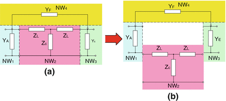
It is possible to convert a general CBDPN configuration to a general Pi network configuration as depicted in Fig. 9.7. To do this conversion, we need to take the following 4 steps.

• 1. Step 1: decomposing the CBDPN into 4 sub-network as shown in Fig. 9.24a, and taking sub-network NW2 out from the CBDPN as shown in Fig. 9.24b.

  Fig. 9.24

  

  Decomposing CBDPN

Where we have

$$ {Y}_A={G}_A+j{B}_A=\frac{1}{R_A}+j\omega \cdot {C}_A $$

(9.44)

$$ {Y}_E={G}_E+j{B}_E=\frac{1}{R_E}+j\omega \cdot {C}_E $$

(9.45)

$$ {Y}_F={G}_F+j{B}_F=\frac{1}{R_F}+j\omega \cdot {C}_F $$

(9.46)

$$ {Z}_C=\frac{1}{Y_C},\kern1.75em \mathrm{and}\kern1.5em {Y}_C={G}_C+j{B}_C=\frac{1}{R_C}+j\omega \cdot {C}_C $$

(9.47)

and

$$ {Z}_L={R}_L+j{X}_L $$

(9.48)

$$ \omega =2\pi f $$

f is operation frequency.

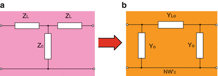
• 2. Step 2: converting the NW2 T type network to a Pi type network as given in Fig. 9.25. The corresponding conversion formulas are expressed by (9.49)–(9.50).

  Fig. 9.25

  

  Converting a T type network to a Pi type network (a) T Network (b) Pi Network

$$ {Y}_o=\frac{1}{Z_L+2{Z}_C}=\frac{Y_C^2\left[\left({R}_L{Y}_C^2+2{G}_C\right)-j\left({Y}_c^2{X}_L-2{B}_C\right)\right]}{{\left({R}_L{Y}_C^2+2{G}_C\right)}^2+{\left({X}_L{Y}_C^2-2{B}_C\right)}^2} $$

(9.49)

and

$$ {Y}_{Lo}=\frac{Y_o{Z}_C}{Z_L}={Y}_o\frac{\left({R}_L{G}_C-{X}_L{B}_C\right)-j\left({R}_L{B}_C+{X}_L{G}_C\right)}{Y_C^2{Z}_L^2} $$

(9.50)

where

$$ {Y}_C^2={Y}_C\cdot {Y}_C^{*}={G}_C^2+{B}_C^2 $$

(9.51)

$$ {Z}_L^2={Z}_L\cdot {Z}_L^{*}={R}_L^2+{X}_L^2 $$

(9.52)

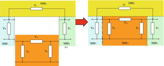
• 3. Step 3: replacing NW2 T type sub-network in CBDPN by the converted Pi type sub-network as shown in Fig. 9.26.

  Fig. 9.26

  

  Replacing NW2 T sub-network by Pi type sub-network

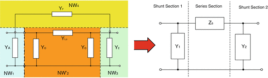
• 4. Step 4: merging the corresponding shunt admittances into Y ₁ and Y ₂ of the Pi network to form the Pi network tuner as depicted in Fig. 9.27. The conversion formulas are given by (9.41)–(9.43).

  Fig. 9.27

  

  Forming a MEMS Pi network tuner

$$ {Y}_1={Y}_A+{Y}_o $$

(9.41)

$$ {Y}_2={Y}_E+{Y}_o $$

(9.42)

and

$$ {Z}_S=\frac{1}{Y_{Lo}+{Y}_F} $$

(9.43)

When G _A  = G _C  = G _E  = G _F  = 0 and R _L  = 0, we have the following formulas:

$$ {C}_1={C}_A+{C}_o={C}_A+\frac{C_C}{2-{\omega}^2L{C}_C} $$

(9.53)

$$ {C}_2={C}_E+{C}_o={C}_E+\frac{C_C}{2-{\omega}^2L{C}_C} $$

(9.54)

$$ {C}_S={C}_F $$

(9.55)

and

$$ {L}_S={L}_o=\left(2-{\omega}^2L{C}_C\right)\cdot L $$

(9.56)

Appendix 2: Calculations of T-Network Elements from S-Parameter Measurements

The network in the middle of the CBDPN is a T type network with two series connected inductors and one shunt capacitor in the middle. The generalized T type network configuration is presented in Fig. 9.28. Where the series impedances Z ₁ and Z _2, and the shunt admittance Y _S can be

Fig. 9.28

Generalized T type network

$$ {Z}_1={R}_1+j{X}_2 $$

(A2.1)

$$ {Z}_2={R}_2+j{X}_2 $$

(A2.2)

and

$$ {Y}_S={G}_S+j{B}_S $$

(A2.3)

The cascaded ABCD matrix of the T type network is

$$ \begin{array}{l}{\left[\begin{array}{cc}\hfill A\hfill & \hfill B\hfill \\ {}\hfill C\hfill & \hfill D\hfill \end{array}\right]}_T={\left[\begin{array}{cc}\hfill {A}_1\hfill & \hfill {B}_1\hfill \\ {}\hfill {C}_1\hfill & \hfill {D}_1\hfill \end{array}\right]}_{series\_1}{\left[\begin{array}{cc}\hfill {A}_S\hfill & \hfill {B}_S\hfill \\ {}\hfill {C}_S\hfill & \hfill {D}_S\hfill \end{array}\right]}_{Shunt}{\left[\begin{array}{cc}\hfill {A}_2\hfill & \hfill {B}_2\hfill \\ {}\hfill {C}_2\hfill & \hfill {D}_2\hfill \end{array}\right]}_{series\_2}\\ {}\kern4em =\left[\begin{array}{cc}\hfill 1\hfill & \hfill {Z}_1\hfill \\ {}\hfill 0\hfill & \hfill 1\hfill \end{array}\right]\cdot \left[\begin{array}{cc}\hfill 1\hfill & \hfill 0\hfill \\ {}\hfill {Y}_S\hfill & \hfill 1\hfill \end{array}\right]\cdot \left[\begin{array}{cc}\hfill 1\hfill & \hfill {Z}_2\hfill \\ {}\hfill 0\hfill & \hfill 1\hfill \end{array}\right]=\left[\begin{array}{cc}\hfill 1+{Z}_1{Y}_S\hfill & \hfill {Z}_1+{Z}_2+{Z}_1{Z}_2{Y}_S\hfill \\ {}\hfill {Y}_S\hfill & \hfill 1+{Z}_2{Y}_S\hfill \end{array}\right]\end{array} $$

(A2.4)

In this case, we have the elements of the T-network ABCD matrix to be

$$ A=1+{Z}_1{Y}_S $$

(A2.5)

$$ B={Z}_1+{Z}_2+{Z}_1{Z}_2{Y}_S $$

(A2.6)

$$ C={Y}_S $$

(A2.7)

and

$$ D=1+{Z}_2{Y}_S $$

(A2.8)

We know the relationship between S-parameters and A, B, C, and D is

$$ {S}_{11}=\frac{A{Z}_o+B-C{Z}_o^2-D{Z}_o}{\Delta} $$

(A2.9)

$$ {S}_{12}=\frac{2\left( AD-BC\right){Z}_o}{\Delta}=\frac{2{Z}_o}{\Delta}\kern1em \mathrm{since}\ AD-BC=1 $$

(A2.10)

$$ {S}_{21}=\frac{2{Z}_o}{\Delta} $$

(A2.11)

and

$$ {S}_{22}=\frac{-A{Z}_o+B-C{Z}_o^2+D{Z}_o}{\Delta} $$

(A2.12)

where

$$ \Delta =A{Z}_o+B+C{Z}_o^2+D{Z}_o $$

(A2.13)

$$ {Z}_o=50\Omega $$

Substituting (A2.5)–(A2.7) into (A2.9)–(A2.13) and after manipulating, we obtain

$$ {S}_{11}=\frac{\left(\overline{Z_1}+\overline{Z_2}\right)+\left[\overline{Z_1}-\overline{Z_2}+\overline{Z_1}\overline{Z_2}-1\right]\cdot \overline{Y_S}}{2+\overline{Z_1}+\overline{Z_2}+\left(1+\overline{Z_1}+\overline{Z_2}+\overline{Z_1}\overline{Z_2}\right)\cdot \overline{Y_S}} $$

(A2.14)

$$ {S}_{12}={S}_{21}=\frac{2}{2+\overline{Z_1}+\overline{Z_2}+\left(1+\overline{Z_1}+\overline{Z_2}+\overline{Z_1}\overline{Z_2}\right)\cdot \overline{Y_S}} $$

(A2.15)

and

$$ {S}_{22}=\frac{\left(\overline{Z_1}+\overline{Z_2}\right)+\left[\overline{Z_2}-\overline{Z_1}+\overline{Z_1}\overline{Z_2}-1\right]\cdot \overline{Y_S}}{2+\overline{Z_1}+\overline{Z_2}+\left(1+\overline{Z_1}+\overline{Z_2}+\overline{Z_1}\overline{Z_2}\right)\cdot \overline{Y_S}} $$

(A2.16)

where

$$ \overline{Z_1}=\frac{Z_1}{Z_o},\kern1.5em \overline{Z_2}=\frac{Z_2}{Z_o},\kern0.75em \mathrm{and}\kern0.75em \overline{Y_S}={Y}_S\cdot {Z}_o $$

(A2.17)

It is possible to solve equations (A2.14)–(A2.16) since they only contain three variables, $\overline{Z_1}$, $\overline{Z_2}$, and $\overline{Y_S}$. To do so, we need to modify the equation set (A2.14)–(A2.16) as follows. First we recognize that the denominator of equations (A2.14)–(A2.16) right side can be determined by utilizing (A2.15) and it has a form as

$$ 2+\overline{Z_1}+\overline{Z_2}+\left(1+\overline{Z_1}+\overline{Z_2}+\overline{Z_1}\overline{Z_2}\right)\cdot \overline{Y_S}=\frac{2}{S_{21}} $$

(A2.18)

We substitute (A2.18) into (A2.14) and (A2.16), respectively, and obtain equations (9.153) and (9.154).

$$ \left(\overline{Z_1}+\overline{Z_2}\right)+\left[\left(\overline{Z_1}-\overline{Z_2}\right)+\overline{Z_1}\overline{Z_2}-1\right]\cdot \overline{Y_S}=\frac{2{S}_{11}}{S_{21}} $$

(A2.19)

and

$$ \left(\overline{Z_1}+\overline{Z_2}\right)+\left[\left(\overline{Z_2}-\overline{Z_1}\right)+\overline{Z_1}\overline{Z_2}-1\right]\cdot \overline{Y_S}=\frac{2{S}_{22}}{S_{21}} $$

(A2.20)

Secondly, adding (A2.19) and (A2.20) on both sides and making subtraction of (A2.19) and (A2.20) from (A2.18), separately, we derive three equations (A2.21)–(A2.23).

$$ \overline{Z_1}+\overline{Z_2}+\left(\overline{Z_1}\overline{Z_2}-1\right)\cdot \overline{Y_S}=\frac{S_{11}+{S}_{22}}{S_{21}} $$

(A2.21)

$$ \left(1+\overline{Z_2}\right)\cdot \overline{Y_S}+1=\frac{1-{S}_{11}}{S_{21}} $$

(A2.22)

and

$$ \left(1+\overline{Z_1}\right)\cdot \overline{Y_S}+1=\frac{1-{S}_{22}}{S_{21}} $$

(A2.23)

Thirdly, from (A2.22) and (A2.23) we can express $\overline{Z_1}$ and $\overline{Z_2}$ as a function of $\overline{Y_S}$.

$$ \overline{Z_1}=\frac{1-{S}_{22}-{S}_{21}\left(1+\overline{Y_S}\right)}{S_{21}\overline{Y_S}} $$

(A2.24)

and

$$ \overline{Z_2}=\frac{1-{S}_{11}-{S}_{21}\left(1+\overline{Y_S}\right)}{S_{21}\overline{Y_S}} $$

(A2.25)

Finally, we solve equation set (A2.21)–(A2.23) by plugging (A2.24) and (A2.25) into (A2.21), and $\overline{Y_S}$ has a solution as

$$ \overline{Y_S}=\frac{1-{S}_{11}-{S}_{22}+{S}_{11}{S}_{22}-{S}_{21}^2}{2{S}_{21}} $$

(9.57)

From (A2.24) to (9.57), we obtain $\overline{Z_1}$ and $\overline{Z_2}$ solutions as.

$$ \overline{Z_1}=\frac{1+{S}_{11}-{S}_{22}-2{S}_{21}-\left({S}_{11}{S}_{22}-{S}_{21}^2\right)}{1-{S}_{11}-{S}_{22}+\left({S}_{11}{S}_{22}-{S}_{21}^2\right)} $$

(9.58)

and

$$ \overline{Z_2}=\frac{1-{S}_{11}+{S}_{22}-2{S}_{21}-\left({S}_{11}{S}_{22}-{S}_{21}^2\right)}{1-{S}_{11}-{S}_{22}+\left({S}_{11}{S}_{22}-{S}_{21}^2\right)} $$

(9.59)

In the case of the network being symmetric, i.e., $\overline{Z_1}=\overline{Z_2}=\overline{Z}$, we have solutions in (9.60) and (9.61).

$$ \overline{Y_S}=\frac{{\left(1-{S}_{11}\right)}^2-{S}_{21}^2}{2{S}_{21}} $$

(9.60)

and

$$ \overline{Z}=\frac{1-2{S}_{21}-\left({S}_{11}^2-{S}_{21}^2\right)}{{\left(1-{S}_{11}\right)}^2-{S}_{21}^2} $$

(9.61)

S_11, S₂₂, and S₂₁ are usually complex numbers and therefore the solutions, $\overline{Z_1}$, $\overline{Z_2}$ and $\overline{Y_S}$ are complex number as well. Their real and imaginary parts are equal to the corresponding parts of (9.57)–(9.61) right sides, respectively. The solutions given in (9.57)–(9.61) are normalized to Z _o  = 50 Ω. The true values of Y ₁ , Y ₂ , and Z _S result from the following equations.

$$ {Z}_1=\overline{Z_1}{Z}_o={R}_1+j{X}_1,\kern0.75em {Z}_2=\overline{Z_2}{Z}_o={R}_2+j{X}_2,\kern0.75em \mathrm{and}\kern0.75em {Y}_S=\frac{\overline{Z_S}}{Z_o}={G}_S+j{B}_S $$

(9.62)

Appendix 3: Shunt Capacitor and Its Q Calculations from Measured S-Parameters

The capacitance and loss of a capacitor at RF can be obtained by using a shunt network as depicted in Fig. 9.29a and through S-parameter measurements. Actually, the capacitance and its loss are calculated from the measured S-parameters of the shunt network instead of directly obtained from the measurement. To drive the calculation formulas it is better to modify Fig. 9.29a into Fig. 9.29b, where

Fig. 9.29

A Shunt 2-port network for Q measurement of Capacitor

$$ Y=G+jB=\frac{1}{R}+j\omega C. $$

(A3.1)

In (A3.1), ω = 2πf and f is operation frequency in Hz. The Q factor of the shunt capacitor is

$$ Q=\frac{B}{G}=\omega C\cdot R $$

(A3.2)

Figure 9.29b network can be characterized by using an ABCD matrix as (A3.3).

$$ \left[\begin{array}{cc}\hfill A\hfill & \hfill B\hfill \\ {}\hfill C\hfill & \hfill D\hfill \end{array}\right]=\left[\begin{array}{cc}\hfill 1\hfill & \hfill 0\hfill \\ {}\hfill Y\hfill & \hfill 1\hfill \end{array}\right] $$

(A3.3)

Utilizing conversions from ABCD matrix to S matrix and considering the symmetry of this network, we have

$$ {S}_{11}={S}_{22}=\frac{A{Z}_o+B-C{Z}_o^2-D{Z}_o}{A{Z}_o+B+C{Z}_o^2+D{Z}_o}=\frac{-Y\cdot {Z}_o^2}{2{Z}_o+Y\cdot {Z}_o^2}=-\frac{\overline{Y}}{2+\overline{Y}} $$

(A3.4)

and

$$ {S}_{21}={S}_{12}=\frac{2\left( AD-BC\right){Z}_o}{A{Z}_o+B+C{Z}_o^2+D{Z}_o}=\frac{2{Z}_o}{2{Z}_o+Y\cdot {Z}_o^2}=\frac{2}{2+\overline{Y}} $$

(A3.5)

where

$$ {Z}_o=50\;\Omega $$

(A3.6)

$$ \overline{Y}=Y\cdot {Z}_o $$

(A3.7)

From (A3.5), we can obtain

$$ 2+\overline{Y}=\frac{2}{S_{21}}. $$

Substituting the above equation into the denominator of (9.169) right side, we derive the following $\overline{Y}$ expression.

$$ \overline{Y}=\frac{-2{S}_{11}}{S_{21}}=\frac{-2\left\{\left[{S}_{11\_\mathrm{R}\mathrm{e}}{S}_{21\_\mathrm{R}\mathrm{e}}+{S}_{11\_\mathrm{I}\mathrm{m}}{S}_{21\_\mathrm{I}\mathrm{m}}\right]+j\left[{S}_{11\_\mathrm{I}\mathrm{m}}{S}_{21\_\mathrm{R}\mathrm{e}}-{S}_{11\_\mathrm{R}\mathrm{e}}{S}_{21\_\mathrm{I}\mathrm{m}}\right]\right\}}{{\left|{S}_{21}\right|}^2} $$

(A3.8)

where

$$ {\left|{S}_{21}\right|}^2={S}_{21\_\mathrm{R}\mathrm{e}}^2+{S}_{21\_\mathrm{I}\mathrm{m}}^2 $$

(A3.9)

$$ {S}_{11\_\mathrm{R}\mathrm{e}}=\mathrm{R}\mathrm{e}\left({S}_{11}\right)\kern1.25em \mathrm{and}\kern1.25em {S}_{11\_\mathrm{I}\mathrm{m}}=\mathrm{I}\mathrm{m}\left({S}_{11}\right) $$

(A3.10)

$$ {S}_{21\_\mathrm{R}\mathrm{e}}=\mathrm{R}\mathrm{e}\left({S}_{21}\right)\kern1.25em \mathrm{and}\kern1.25em {S}_{21\_\mathrm{I}\mathrm{m}}=\mathrm{I}\mathrm{m}\left({S}_{21}\right) $$

(A3.11)

The normalized Y can be expressed as

$$ \overline{Y}=\overline{G}+j\overline{B}\kern2.5em \mathrm{with}\kern0.5em \overline{G}=G\cdot {Z}_o\kern0.5em \mathrm{and}\kern0.5em \overline{B}=B\cdot {Z}_o $$

(9.63)

and

$$ \overline{G}=-2\frac{S_{11\_\mathrm{R}\mathrm{e}}{S}_{21\_\mathrm{R}\mathrm{e}}+{S}_{11\_\mathrm{I}\mathrm{m}}{S}_{21\_\mathrm{I}\mathrm{m}}}{{\left|{S}_{21}\right|}^2} $$

(9.64)

$$ \overline{B}=-2\frac{S_{11\_\mathrm{I}\mathrm{m}}{S}_{21\_\mathrm{R}\mathrm{e}}-{S}_{11\_\mathrm{R}\mathrm{e}}{S}_{21\_\mathrm{I}\mathrm{m}}}{{\left|{S}_{21}\right|}^2} $$

(9.65)

From (9.64) and (9.65), we drive the Q factor of the series inductor to be

$$ Q=\frac{\omega C}{G}=\frac{\overline{B}}{\overline{G}}=\frac{S_{11\_\mathrm{I}\mathrm{m}}{S}_{21\_\mathrm{R}\mathrm{e}}-{S}_{11\_\mathrm{R}\mathrm{e}}{S}_{21\_\mathrm{I}\mathrm{m}}}{S_{11\_\mathrm{R}\mathrm{e}}{S}_{21\_\mathrm{R}\mathrm{e}}+{S}_{11\_\mathrm{I}\mathrm{m}}{S}_{21\_\mathrm{I}\mathrm{m}}} $$

(9.66)

and obtain R and C as

$$ R=\frac{1}{G}=-\frac{25\cdot {\left|{S}_{21}\right|}^2}{\left({S}_{11\_\mathrm{R}\mathrm{e}}{S}_{21\_\mathrm{R}\mathrm{e}}+{S}_{11\_\mathrm{I}\mathrm{m}}{S}_{21\_\mathrm{I}\mathrm{m}}\right)}\kern1em \Omega $$

(9.67)

and

$$ B=-\frac{S_{11\_\mathrm{I}\mathrm{m}}{S}_{21\_\mathrm{R}\mathrm{e}}-{S}_{11\_\mathrm{R}\mathrm{e}}{S}_{21\_\mathrm{I}\mathrm{m}}}{25\cdot {\left|{S}_{21}\right|}^2} $$

(9.68)

or

$$ \begin{array}{l}C=-\frac{S_{11\_\mathrm{I}\mathrm{m}}{S}_{21\_\mathrm{R}\mathrm{e}}-{S}_{11\_\mathrm{R}\mathrm{e}}{S}_{21\_\mathrm{I}\mathrm{m}}}{25\cdot \omega \cdot {\left|{S}_{21}\right|}^2}\cdot {10}^{12}\kern1.25em \mathrm{pF}\\ {}\kern1em =\frac{S_{11\_\mathrm{R}\mathrm{e}}{S}_{21\_\mathrm{I}\mathrm{m}}-{S}_{11\_\mathrm{I}\mathrm{m}}{S}_{21\_\mathrm{R}\mathrm{e}}}{25\cdot \omega \cdot {\left|{S}_{21}\right|}^2}\cdot {10}^{12}\kern2em \mathrm{pF}\end{array} $$

(9.69)

Appendix 4: Series Inductor and Its Q Calculations from Measured S-Parameters

The quality factor Q of an inductor can be measured by means of a series two-port network as shown in Fig. 9.30 and the S parameters. In Fig. 9.30a, R represents the loss of the inductor with an inductance L, and the overall impedance of this inductor is

Fig. 9.30

A series two-port network for Q measurement of inductor

$$ Z=R+jX=R+j\omega L. $$

(A4.1)

where ω = 2πf and f is operation frequency in Hz. The network Fig. 9.30a can be equivalently expressed as Fig. 9.30b. The Q factor of this inductor is

$$ Q=\frac{X}{R}=\frac{\omega L}{R} $$

(A4.2)

The network of Fig. 9.30b can be simply described by an ABCD matrix as (A4.3).

$$ \left[\begin{array}{cc}\hfill A\hfill & \hfill B\hfill \\ {}\hfill C\hfill & \hfill D\hfill \end{array}\right]=\left[\begin{array}{cc}\hfill 1\hfill & \hfill Z\hfill \\ {}\hfill 0\hfill & \hfill 1\hfill \end{array}\right] $$

(A4.3)

Utilizing conversions from ABCD matrix to S matrix and considering the symmetry of this network, we have

$$ {S}_{11}={S}_{22}=\frac{A{Z}_o+B-C{Z}_o^2-D{Z}_o}{A{Z}_o+B+C{Z}_o^2+D{Z}_o}=\frac{Z}{2{Z}_o+Z}=\frac{\overline{Z}}{2+\overline{Z}} $$

(A4.4)

and

$$ {S}_{21}={S}_{12}=\frac{2\left( AD-BC\right){Z}_o}{A{Z}_o+B+C{Z}_o^2+D{Z}_o}=\frac{2{Z}_o}{2{Z}_o+Z}=\frac{2}{2+\overline{Z}} $$

(A4.5)

where

$$ {Z}_o=50\;\Omega $$

(A4.6)

$$ \overline{Z}=\frac{Z}{Z_o} $$

(A4.7)

From (A4.5), we can obtain

$$ 2+\overline{Z}=\frac{2}{S_{21}}. $$

Substituting the above equation into the denominator of (A4.4) right side, we derive the following $\overline{Z}$ expression.

$$ \overline{Z}=\frac{2{S}_{11}}{S_{21}}=\frac{2\left\{\left[{S}_{11\_\mathrm{R}\mathrm{e}}{S}_{21\_\mathrm{R}\mathrm{e}}+{S}_{11\_\mathrm{I}\mathrm{m}}{S}_{21\_\mathrm{I}\mathrm{m}}\right]+j\left[{S}_{11\_\mathrm{I}\mathrm{m}}{S}_{21\_\mathrm{R}\mathrm{e}}-{S}_{11\_\mathrm{R}\mathrm{e}}{S}_{21\_\mathrm{I}\mathrm{m}}\right]\right\}}{{\left|{S}_{21}\right|}^2} $$

(A4.8)

where

$$ {\left|{S}_{21}\right|}^2={S}_{21\_\mathrm{R}\mathrm{e}}^2+{S}_{21\_\mathrm{I}\mathrm{m}}^2 $$

(A4.9)

$$ {S}_{11\_\mathrm{R}\mathrm{e}}=\mathrm{R}\mathrm{e}\left({S}_{11}\right)\kern1.25em \mathrm{and}\kern1.25em {S}_{11\_\mathrm{I}\mathrm{m}}=\mathrm{I}\mathrm{m}\left({S}_{11}\right) $$

(A4.10)

$$ {S}_{21\_\mathrm{R}\mathrm{e}}=\mathrm{R}\mathrm{e}\left({S}_{21}\right)\kern1.25em \mathrm{and}\kern1.25em {S}_{21\_\mathrm{I}\mathrm{m}}=\mathrm{I}\mathrm{m}\left({S}_{21}\right) $$

(A4.11)

The normalized Z can be expressed as

$$ \overline{Z}=\overline{R}+j\overline{X}\kern2.5em \mathrm{with}\kern0.5em \overline{R}=\frac{R}{Z_o}\kern0.5em \mathrm{and}\kern0.5em \overline{X}=\frac{X}{Z_o} $$

(9.70)

and

$$ \overline{R}=2\frac{S_{11\_\mathrm{R}\mathrm{e}}{S}_{21\_\mathrm{R}\mathrm{e}}+{S}_{11\_\mathrm{I}\mathrm{m}}{S}_{21\_\mathrm{I}\mathrm{m}}}{{\left|{S}_{21}\right|}^2} $$

(9.71)

$$ \overline{X}=2\frac{S_{11\_\mathrm{I}\mathrm{m}}{S}_{21\_\mathrm{R}\mathrm{e}}-{S}_{11\_\mathrm{R}\mathrm{e}}{S}_{21\_\mathrm{I}\mathrm{m}}}{{\left|{S}_{21}\right|}^2} $$

(9.72)

From (9.71) and (9.72), we drive the Q of the series inductor to be

$$ Q=\frac{\omega L}{R}=\frac{\overline{X}}{\overline{R}}=\frac{S_{11\_\mathrm{I}\mathrm{m}}{S}_{21\_\mathrm{R}\mathrm{e}}-{S}_{11\_\mathrm{R}\mathrm{e}}{S}_{21\_\mathrm{I}\mathrm{m}}}{S_{11\_\mathrm{R}\mathrm{e}}{S}_{21\_\mathrm{R}\mathrm{e}}+{S}_{11\_\mathrm{I}\mathrm{m}}{S}_{21\_\mathrm{I}\mathrm{m}}} $$

(9.73)

and obtain R and L as

$$ R=\frac{S_{11\_\mathrm{R}\mathrm{e}}{S}_{21\_\mathrm{R}\mathrm{e}}+{S}_{11\_\mathrm{I}\mathrm{m}}{S}_{21\_\mathrm{I}\mathrm{m}}}{{\left|{S}_{21}\right|}^2}\cdot 100\kern1.25em \Omega $$

(9.74)

and

$$ X=\frac{S_{11\_\mathrm{I}\mathrm{m}}{S}_{21\_\mathrm{R}\mathrm{e}}-{S}_{11\_\mathrm{R}\mathrm{e}}{S}_{21\_\mathrm{I}\mathrm{m}}}{{\left|{S}_{21}\right|}^2}\cdot 100 $$

(9.75)

or

$$ L=\frac{S_{11\_\mathrm{I}\mathrm{m}}{S}_{21\_\mathrm{R}\mathrm{e}}-{S}_{11\_\mathrm{R}\mathrm{e}}{S}_{21\_\mathrm{I}\mathrm{m}}}{\omega \cdot {\left|{S}_{21}\right|}^2}\cdot {10}^{11}\kern1.25em \mathrm{n}\mathrm{H} $$

(9.76)