The Steady Electric Current

Abstract

In the previous four chapters, we discussed the electrostatic field and its applications. The only reference to time was in the fact that whenever charges are placed in a conductor, they move until a steady state charge distribution is obtained. However, no attempt was made to characterize their motion or any effects this might have on fields.

I believe there are 15,747,724,136,275,002,577,605,653,961,181,555,468,044,717,914,527, 116,709,366,231,425,076,185,631,031,296 protons in the universe and the same number of electrons.

—Sir Arthur Eddington (1882–1944), physicist

The Philosophy of Physical Science (Cambridge, 1939)

Problems

7.1.1 Convection and Conduction Current

• 7.1 Current and Charge in a Battery. Consider a 12 V car battery rated at 100 A⋅h. This battery can supply a current of 100 A for an hour:

  • (a) How much charge can the battery supply?

  • (b) What must be the area of a parallel plate capacitor, with plates separated a distance d = 0.01 mm and relative permittivity of 4 for the dielectric between the plates to supply the same charge as the battery in (a)?

• 7.2 Application: Convection Current. The solar wind is a stream of mostly protons emitted by the Sun as part of its normal reaction. The particles move at about 500 km/s and, at the Earth’s orbit, the particle density is about 10⁶ protons per m³. Most of these protons are absorbed in the upper atmosphere and never reach the surface of the Earth:

  • (a) Taking the radius of the Earth as 6,400 km and the charge of the proton as 1.6 × 10⁻¹⁹ C, calculate the current intercepting the globe if these charges were not absorbed in the atmosphere.

  • (b) During a solar flare, the solar wind becomes much more intense. The velocity increases to 1,000 km/s (typical) and the number of particles increases to about 10⁷ protons/m³. Calculate the current intercepting the globe during a solar flare.

• 7.3 Application: Velocity of Electrons in Conductors. The free electron density in copper is 8 × 10²⁸ electrons/m³. A copper cable, 30 mm in diameter, carries a current of 3000 A. Find the drift velocity of the electrons.

• 7.4 Drift Velocity and Electric Field Intensity in Conductors. A copper conductor with conductivity σ = 5.7 × 10⁷ S/m carries a current of 10 A. The conductor has a diameter of 2 mm. Calculate:

  • (a) The electric field intensity inside the conductor.

  • (b) The average drift velocity of electrons in the conductor assuming a free electron density of 8 × 10²⁸ electrons/m³.

• 7.5 Electric Field Due to a Charged Beam. A cylindrical electron beam consists of a uniform volume charge density moving at a constant axial velocity v ₀ = 5 × 10⁶ m/s. The total current carried by the beam is I ₀ = 5 mA and the beam has a diameter of 1 mm. Assuming a uniform distribution of charges within the beam’s volume, calculate the electric field intensity inside and outside the electron beam.

7.1.2 Conductivity and Resistance

• 7.6 Carrier Velocity and Conductivity. A power device is made of silicon and carries a current of 100 A. The size of the device is 10 mm × 10 mm and is 1 mm thick. The potential drop on the device is 0.6 V, measured across the thickness of the device:

  • (a) What is the conductivity of the silicon used?

  • (b) If the velocity of the carriers is 2,000 m/s, how many free charges (electrons) must be present in the device at all times?

• 7.7 Lossy Coaxial Cable. In a coaxial cable of length L, the inner conductor is of radius a [m] and the outer conductor of radius b [m], and these are separated by a lossy dielectric with permittivity ε [F/m] and conductivity σ [S/m]. A DC source, V [V], is connected with the positive side to the outer conductor of the cable. Neglecting edge effects determine:

  • (a) The electric field intensity in the dielectric.

  • (b) The current density in the dielectric.

  • (c) The total current flowing from outer to inner conductor.

  • (d) The resistance between the outer and inner conductors.

• 7.8 Conductivity. A conductor was found in an application, but it is not known what type of material it is. Since it is required to replace the conductor with a conductor of equivalent properties, the conductivity of the material must be determined. The length of the conductor is 100 m and its diameter 1.2 mm. A 12 V source is connected across the conductor and the current is measured as 0.1 A. What is an appropriate material conductivity to use in this application?

• 7.9 Resistance in Layered Conductors. A cylindrical conductor, 1 m long, is made of layered materials as shown in Figure 7.31

  

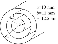
  Figure 7.31

  . The inner layer is copper, the intermediate layer is brass, and the outer layer is a thin coating of nichrome, used for appearances’ sake. Use conductivity data from Table 7.1:

  • (a) Calculate the resistance of the conductor before coating with nichrome, as measured between the two flat bases of the cylinder.

  • (b) What is the percentage change in resistance of the conductor due to the nichrome coating?

• 7.10 Application: Temperature Dependency of Resistance. Conductivity of copper varies with temperature as σ = σ ₀ /[1 + α(T − T ₀)], where α = 0.0039/°C for copper, T is the actual temperature and T ₀ is the temperature at which σ ₀ is known (usually 20°C). A cylindrical copper conductor of radius 10mm and length 0.3 m passes through a wall as shown in Figure 7.32

  

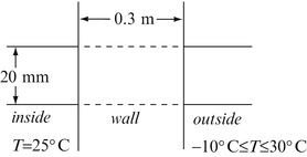
  Figure 7.32

  . The temperature inside is constant at 25°C and the temperature outside varies from 30° C in summer and −10°C in winter. Conductivity of copper is σ ₀ = 5.7 × 10⁷ S/m at T ₀ = 20°C. The temperature distribution along the bar is linear:

  • (a) What is the resistance of the conductor bar section embedded in the wall in summer?

  • (b) What is the resistance of the conductor bar section embedded in the wall in winter?

  • (c) How can this conductor be used to measure the temperature difference between outside and inside?

• 7.11 Application: Temperature Sensor. It is required to design a device to measure the temperature of an internal combustion engine. The minimum temperature expected is −30°C and maximum temperature is that of boiling water. A copper wire is wound in the form of a coil and is enclosed in a watertight enclosure which is immersed in the coolant of the engine. If the copper wire is 10 m long, and 0.1 mm in diameter, calculate the minimum and maximum resistance of the sensor provided its conductivity is given by σ = σ ₀ /[1 + α(T − T ₀)], where α = 0.0039/°C, σ ₀ = 5.7 × 10⁷ S/m is the conductivity at 20° C, and T ₀ = 20°C. Assume the dimensions of the wire do not change with temperature.

• 7.12 Application: Measurement of Conductivity. A very simple (and not very accurate) method of measuring conductivity of a solid material is to make a cylinder of the material and place it between two cylinders of known dimensions and conductivity, as shown in Figure 7.33

  

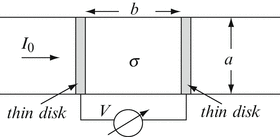
  Figure 7.33

  . A current source, with constant current I ₀ [A], is connected to the three cylinders. A voltmeter is connected to two very thin disks made of silver. The voltage read is directly proportional to the resistance of the cylinder, and since the dimensions are known, the conductivity of the material can be related to the potential:

  • (a) Calculate the conductivity of the material as a function of dimensions and potential. Use I ₀ = 1 A, a = 10 mm, b = 100 mm.

  • (b) What are the implicit assumptions in this measurement?

• 7.13 Measurement of Conductivity. A method of measuring conductivity of fluids is to construct a cylinder and drill a hole at the center of the cylinder. Both ends are plugged with cylindrical plugs of known length and of the same conductivity as the cylinder (Figure 7.34a ). Assuming the conductivity of the cylinder is σ ₀ [S/m] and dimensions are as shown, calculate the resistance of the device. Now, one plug is removed and the hollow space is filled with fluid as shown in Figure 7.34b. If the resistance of the device is now lower by 10%, what is the conductivity of the fluid?

  

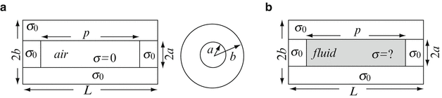
  Figure 7.34

• 7.14 Calculation of Resistance. A sphere made of a conducting material with conductivity σ [S/m] is connected in a circuit as shown in Figure 7.35a

  

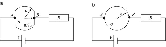
  Figure 7.35

  . For connection purposes, the sphere is trimmed and connections made to the flat surfaces created by the cuts. The resistance R [Ω] and source voltage V [V] are known:

  • (a) Calculate the potential on the sphere (between points A and B) in terms of the known parameters.

  • (b) Suppose that instead of cutting the sphere as in Figure 7.35a, the connections are made as in Figure 7.35b. Show that the resistance of the sphere cannot be calculated exactly and comment on the physical meaning of this result.

• 7.15 Potential Difference and Resistance. Three cylinders are attached as shown in Figure 7.36. A current I passes through the cylinders. If σ ₁, σ ₂, and σ ₃ [S/m] are the conductivities of the cylinders, calculate the potential difference on the three cylinders. Assume current densities are uniform in each cylinder.

  

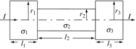
  Figure 7.36

• 7.16 Nonhomogeneous Conductivity. A block of material with dimensions as shown in Figure 7.37 has conductivity: σ = σ ₀ + ax ² [S/m], where x = 0 at the left end of the block. A current I [A] passes through the block. σ ₀ is a constant. Calculate the resistance of the block and the potential difference between the two ends of the block.

  

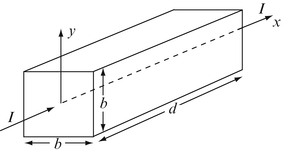
  Figure 7.37

• 7.17 Potential Difference and Resistance. A conducting sphere of radius a [m], with conductivity σ [S/m], is cut into two hemispheres. Then, each hemisphere is trimmed so that it has a flat surface on top and the two sections are connected as shown in Figure 7.38

  

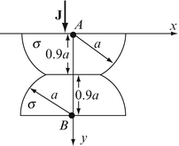
  Figure 7.38

  . A uniform current density J [A/m²] crosses the upper flat surface as shown:

  • (a) Calculate the potential difference between A and B.

  • (b) Compare the result in (a) with that obtained in Problem 7.14a.

• 7.18 Application: Ground Resistance of Electrodes. A ground electrode is built in the form of a hemisphere, of radius a = 0.1 m, buried in the ground, flush with the surface as shown in Figure 7.39. Calculate the contact resistance (resistance between the wire and surrounding ground). You may assume the ground is a uniform medium semi-infinite in extent, with conductivity σ = 0.1 S/m. Hint Calculate the resistance between the hemisphere and a concentric conducting surface at infinity. Note: This is an important calculation in design of lightning and power fault protection systems.

  

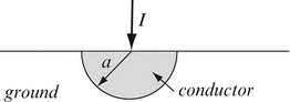
  Figure 7.39

• 7.19 Application: Measurement of Soil Resistivity for Mineral Prospecting. The measurement of soil resistivity (or its reciprocal, conductivity) is an important activity in prospecting for minerals. Usually two or more electrodes are inserted in the ground and the current measured for a known voltage. The ground resistivity can then be correlated with the presence of minerals.

  Two conducting electrodes, each made in the form of a half sphere, one of radius a, the second of radius b, are buried in the ground flush with the surface (Figure 7.40 ). The horizontal distance between the centers of the electrodes is large so that one electrode does not influence the other (i.e., the current around one electrode is not distorted by the proximity of the other). If a battery of voltage V ₀ is connected as shown and a current I ₀ is measured, calculate the conductivity of the soil. You may assume that the ground is semi-infinite. Assume the conductivity of the electrodes is much higher than that of the soil and hence their resistance can be neglected.

  

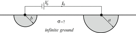
  Figure 7.40

7.1.3 Power Dissipation and Joule’s Law

• 7.20 Application: Series and Parallel Loads. The early electric distribution for lighting (Edison’s system) was in series. All electric bulbs were connected in series and the source voltage was raised to the required value. Today’s systems are almost always in parallel. Suppose you wanted to calculate which system is more economical in terms of power loss for street lighting. A street is 1 km long and a light bulb is placed every 50 m (total of 20 bulbs), each bulb rated at 240 V, 500 W:

  • (a) What is the minimum wire thickness required for the parallel and series connections (copper, σ = 5.7 × 10⁷ S/m) if the current density cannot exceed 10⁶ A/m² and the wires must be of the same thickness everywhere?

  • (b) The wire calculated in (a) is used. Calculate: (1) The total weight of copper used for the series and parallel systems (copper weighs approximately 8 tons/m³). (2) Total power loss in the copper wires. (3) Which system is more economical in terms of amount of copper needed and in terms of power loss?

  • (c) What are your conclusions from the calculations above?

• 7.21 Application: Resistance and Power in Faulty Cables. An underwater cable is made as a coaxial cable with internal conductor of diameter a = 10 mm and an external conductor of diameter b = 20 mm (see Figure 7.41

  

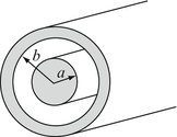
  Figure 7.41

  ). The cable is made of a superconducting material (σ = ∞), is 10 km long, and operates at 480 V. Because of a leak, seawater (σ = 4 S/m) entered the cable, filling the space between the conductors:

  • (a) What is the resistance seen by a generator connected to the cable at one end?

  • (b) How much power is dissipated in the seawater inside the cable?

• 7.22 Application: Bimetal Conductor. A conductor is made of two materials as shown in Figure 7.42. This is typical of bimetal devices. The device is connected to a voltage source:

  

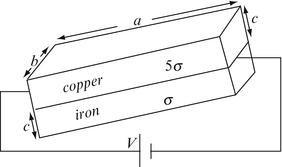
  Figure 7.42

  • (a) Calculate the current density in each material.

  • (b) Calculate the total power dissipated in each material.

  • (c) Assuming that each material has the same coefficient of expansion and the same power dissipating capability, which way will the bimetal device bend? Explain.

• 7.23 Series and Parallel Resistances. An antenna element is made of a hollow aluminum tube, L = 800 mm long, with inner diameter a = 10 mm and outer diameter b = 12 mm. For operational reasons, it becomes necessary to lengthen the antenna to 1,200 mm. To do so, it is proposed to use the same tube but add a cylindrical solid graphite coupler that fits in the tube with a shoulder to support the extension as shown in Figure 7.43

  

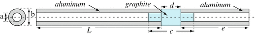
  Figure 7.43

  . Conductivity of aluminum is σ _a  = 3.6 × 10⁷ S/m and that of graphite is σ _g  = 10⁴ S/m. The coupler’s dimensions are c = 120 mm, d = 40 mm and each of the sections that fit inside the tube is 40 mm long. The extension tube is e = 360 mm long:

  • (a) Calculate the change in resistance of the antenna element (resistance is measured between the two ends of the structure) due to the change in the structure.

  • (b) Suppose that because of cost the graphite coupler is replaced with an identical aluminum coupler. What is now the change in resistance?

  Note: The resistance of antennas is an important parameter in antenna efficiency.

• 7.24 Series and Parallel Resistances. Consider again Problem 7.23. After fitting the coupler and the extension, it became evident that the structure is not sufficiently strong. To improve its strength, a graphite tube is added over the graphite coupler as shown in Figure 7.44

  

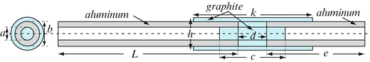
  Figure 7.44

  . The graphite tube is k = 200 mm long and has inner diameter equal to the outer diameter of the tube (b = 12 mm) and outer diameter h = 16 mm. The tube is centered over the coupler. Given the dimensions and material properties, calculate:

  • (a) The total resistance of the antenna.

  • (b) The total resistance of the antenna if both the coupler and the external tube are made of aluminum.

7.1.4 Continuity and Circuit Laws

• 7.25 Application: Conservation of Charge. A small ion thruster is made in the form of a box with a round opening through which the ions are ejected (Figure 7.45

  

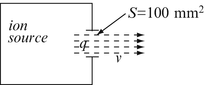
  Figure 7.45

  ). Suppose that by external means (not shown) the ions are ejected at a velocity of 10⁶ m/s, the ions are all positive with charge equal to that of a proton, and the ion density in the ion beam is 10¹⁸ ions/m³. The opening is 100 mm² in area and the beam may be considered to be cylindrical. Calculate:

  • (a) The current in the beam.

  • (b) Discuss the behavior of this current over time.

• 7.26 Conservation of Charge in a Circuit. A capacitor of capacitance C = 1,000 μF is connected in series with a switch and a 12 V battery. The resistance of the wires is 10 Ω, and the wire used in the circuit is 1 mm in diameter. The switch is switched on at t = 0:

  • (a) Show that if you take a volume that includes one plate of the capacitor (see Figure 7.46 ), Kirchhoff’s current law as defined in circuits is not satisfied.

  • (b) Calculate the rate of change of charge on the plate in Figure 7.46.

  • (c) Show that the current cannot be a steady current.

  

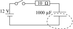
  Figure 7.46

7.1.5 Interface Conditions

• 7.27 Surface Charge Produced by Current. Two cylindrical, lossy dielectrics of radius b [m] but of different conductivities are connected to a potential V [V]. Dimensions and properties are shown in Figure 7.47. Two perfectly conducting cylinders are connected to the two ends for the purpose of connecting to the source. Calculate the total charge at the interface between each two materials (see arrows in Figure 7.47 ).

  

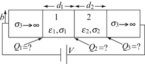
  Figure 7.47

• 7.28 Current and Power in Layered Materials. A copper and an aluminum conductor are connected as shown in Figure 7.48

  

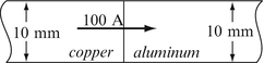
  Figure 7.48

  . Both have a diameter d = 10 mm. A 100 A current flows through the copper conductor as shown. Properties are σ _cu  = 5.7 × 10⁷ S/m and σ _al  = 3.6 × 10⁷ S/m. Calculate:

  • (a) The electric field intensity in copper and in aluminum.

  • (b) The dissipated power density in copper and in aluminum.

• 7.29 Application: Spot Welding of Sheet Stock. In an electric spot welding machine, the electrodes are circular with diameter d = 10 mm. Two sheets of steel are welded together (Figure 7.49

  

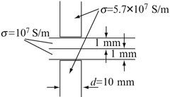
  Figure 7.49

  ). If the power density (in steel) required for welding is 10⁸ W/m³, calculate:

  • (a) The potential difference needed on the steel sheets and the current in the electrodes.

  • (b) The dissipated power density in the electrodes.

  (Assume the weld area equals the cross-sectional area of the electrodes and all current flows in the weld area.)