Introduction

Abstract

The motion of a charged point particle is influenced by electromagnetic fields according to the Lorentz force¹

$$\displaystyle{ \fbox{$\vec{F} = Q\left (\vec{E} +\vec{ u} \times \vec{ B}\right ).$} }$$

(1.1)

Here Q denotes the charge of the particle, and $\vec{E}(\vec{r},t)$ and $\vec{B}(\vec{r},t)$ are the electric field and the magnetic induction vectors, respectively, at a certain time t and at the position $\vec{r}(t)$ of the charge.

These keywords were added by machine and not by the authors. This process is experimental and the keywords may be updated as the learning algorithm improves.

The motion of a charged point particle is influenced by electromagnetic fields according to the Lorentz force¹

$$\displaystyle{ \fbox{$\vec{F} = Q\left (\vec{E} +\vec{ u} \times \vec{ B}\right ).$} }$$

(1.1)

Here Q denotes the charge of the particle, and $\vec{E}(\vec{r},t)$ and $\vec{B}(\vec{r},t)$ are the electric field and the magnetic induction vectors, respectively, at a certain time t and at the position $\vec{r}(t)$ of the charge. In this book, we will alternatively call $\vec{B}$ the magnetic field, since the distinction between $\vec{B}$ and the magnetic field vector $\vec{H}$ is obvious. The vector $\vec{u} = \frac{\mathrm{d}\vec{r}} {\mathrm{d}t}$ is the instantaneous velocity of the point charge.

For the energy gain due to the electromagnetic field, we obtain

$$\displaystyle{\Delta W =\int _{C}\vec{F} \cdot \mathrm{ d}\vec{r} = Q\int _{C}\vec{E} \cdot \mathrm{ d}\vec{r} + Q\int _{C}\left (\frac{\mathrm{d}\vec{r}} {\mathrm{d}t} \times \vec{ B}\right ) \cdot \mathrm{ d}\vec{r},}$$

where C is the flight path of the particle. For the second integral, we obtain

$$\displaystyle{\int _{C}\left (\frac{\mathrm{d}\vec{r}} {\mathrm{d}t} \times \vec{ B}\right ) \cdot \mathrm{ d}\vec{r} =\int _{ t_{1}}^{t_{2} }\left (\frac{\mathrm{d}\vec{r}} {\mathrm{d}t} \times \vec{ B}\right ) \cdot \frac{\mathrm{d}\vec{r}} {\mathrm{d}t}\;\mathrm{d}t = 0,}$$

since two factors of the scalar triple product are equal. Therefore, it is impossible to use magnetic fields to change the energy of the charged particle.² Magnetic fields may be used to deflect particles, but an acceleration in the sense of changing their energy by

$$\displaystyle{ \fbox{$\Delta W = Q\int _{C}\vec{E} \cdot \mathrm{ d}\vec{r} = QV $} }$$

(1.2)

requires electric fields that lead to a voltage

$$\displaystyle{V =\int _{C}\vec{E}(\vec{r},t) \cdot \mathrm{ d}\vec{r} =\int _{ t_{1}}^{t_{2} }\vec{E}(\vec{r}(t),t) \cdot \frac{\mathrm{d}\vec{r}} {\mathrm{d}t}\;\mathrm{d}t.}$$

Please note that we will always define the voltage V to be oriented in the same way as the direction of flight. For acceleration, we need V > 0 in case of Q > 0 (e.g., protons or other positive ions) and V < 0 in case of Q < 0 (e.g., electrons).

The simplest choice of an electric field is a time-independent field, i.e., a DC field. The total energy that may be reached by DC fields, however, is limited by high-voltage sparkovers.

The next logical step to increase the overall voltage would be to use not only one accelerating section but several adjacent ones. This does not solve the problem, however, since either the DC voltages will add up to a voltage that again leads to sparkovers, or—depending on the grounding concept of the sections—DC voltages in the reverse direction will be present, leading to sections with undesired deceleration.

These limits may be exceeded if AC fields are used, especially in the radio frequency (RF) range, because the particles may then gain energy several times. In a linear accelerator, the beam passes different cavities, which may consist of different accelerating cells. In a ring accelerator such as a synchrotron or a storage ring, the particles repeatedly gain energy in the same cavity or in the same number of cavities, since they arrive at the same place after one revolution.

When using RF fields, one still has to make sure that the acceleration that is realized during one-half of the RF period does not lead to a deceleration during the other half of the period. In linear accelerators (LINACs), this may be accomplished by so-called drift tubes, which shield the particles against electric fields with the wrong polarity (cf. [1]). In synchrotrons and storage rings, the particles will be located inside the conducting beam pipe during those time intervals in which the field has the wrong polarity. The electric field may be generated in a so-called ceramic gap. Such a ceramic gap is a short ceramic tube that interrupts the metallic beam pipe. Since its material is nonconducting, a voltage can be induced even though the beam pipe is still evacuated.

Figure 1.1 shows the main elements (cf. [2] for further reading) of a synchrotron or storage ring in a schematic way:

• A metallic beam pipe is evacuated so that flying particles will not hit gas molecules. For storage rings with long storage times (e.g., on the order of several hours), a better vacuum quality is usually required than is to be found in synchrotrons that are used only for comparatively short acceleration phases.

  Fig. 1.1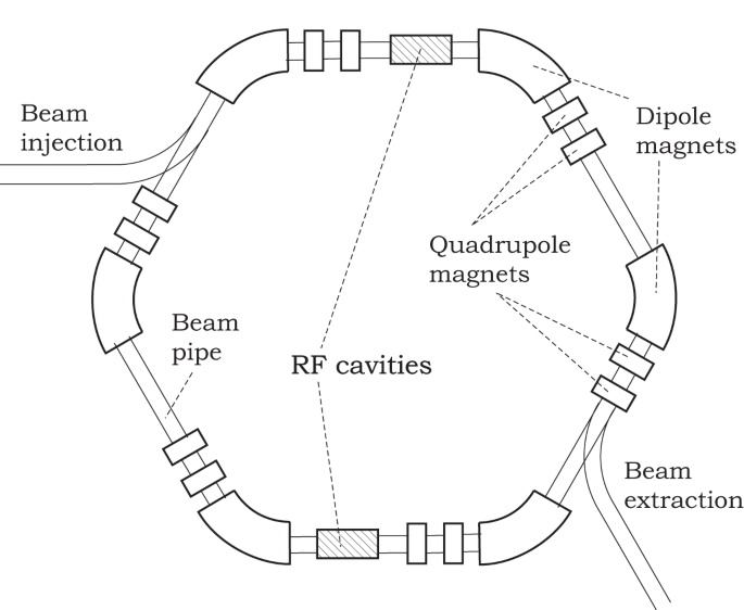

  

  Schematic drawing of a synchrotron

• An injection system is used to deflect the beam (which comes from a linear accelerator or a booster synchrotron) onto its target trajectory. Following the acceleration, which may need thousands of revolutions, the beam is extracted by a similar system. Injection and extraction are shown only schematically in Fig. 1.1.

• Dipole magnets are used to deflect particles in such a way that a closed orbit is realized. Inside a dipole magnet, a constant or slowly varying B field is oriented in the vertical direction so that the beam is bent horizontally. Dipole magnets are therefore the arcs of a synchrotron. They are also called bending magnets.

• Quadrupole magnets are used as focusing elements. A quadrupole magnet leads to transverse focusing in one direction (e.g., in the radial x direction) and to defocusing in the other direction (e.g., in the vertical y direction). Fortunately, the net effect of two quadrupoles the first of which produces focusing in the x direction (and defocusing in the y direction) while the second produces focusing in the y direction (and defocusing in the x direction) is to focus in both directions. Therefore, two (a so-called quadrupole doublet) or three quadrupole magnets (a quadrupole triplet) are typically combined. One also speaks of magnetic quadrupole lenses, since the effect in ion or electron optics is comparable with the effect in light optics.

• In the straight sections of the synchrotron, a set of RF cavities is used to produce the electric field, mentioned above, that is required for the desired energy gain $\Delta W$.

In a synchrotron, there is a specific orbit that is the desired one. Of course, not all particles will follow this orbit precisely, because the ideal situation that all particles have no transverse offset from this reference orbit cannot be realized. However, we may assume that a so-called reference particle will follow the reference orbit.

When the reference particle gains energy in an RF cavity, it is clear that the dipole field B has to be increased to keep the reference particle on the reference orbit (path length l_R for one revolution). One immediately sees that these conditions can be fulfilled only if all parameters—the magnetic dipole field B, the RF voltage amplitude, and the RF frequency—fit together. These parameters have to be varied synchronously, whence the name “synchrotron.”

The reference particle (with reference energy W_R) is also called a synchronous particle. Typically, the energy gain $\Delta W$ in each revolution is small in comparison with the total energy W_R. The desired total energy gain is reached only because of the very large number of revolutions.

We now discuss the effect of the RF cavity on positive charges Q > 0. A sinusoidal RF voltage V (t) is sketched in Fig. 1.2. This voltage is specified by

$$\displaystyle{V =\hat{ V }\;\sin (\varphi _{\mathrm{RF}}),}$$

where the RF phase is given by

$$\displaystyle{ \varphi _{\mathrm{RF}} =\int _{ 0}^{t}\omega _{ \mathrm{RF}}(\tilde{t})\;\mathrm{d}\tilde{t}. }$$

(1.3)

In general, the amplitude $\hat{V }$ and the RF frequency³$f_{\mathrm{RF}} = \frac{\omega _{\mathrm{RF}}} {2\pi }$ are time-dependent quantities.

Fig. 1.2

Phase-focusing principle

Let us assume that a certain level V_R of the electric voltage leads to the “correct” energy gain, i.e., after passing the RF cavity, the particle has an energy that allows it to travel on the desired path in the beam pipe and to “see” the correct voltage V_R the next time it arrives again at the RF cavity. In other words, in each revolution, the reference particle will experience an energy gain that allows it to stay on the reference path. The energy gain $\Delta W$ of the particle is small in comparison with its energy W_R. Also, the relative change in its velocity is small. Therefore, one may regard the RF frequency as constant during several periods, so that

$$\displaystyle{\varphi _{\mathrm{RF}} \approx \omega _{\mathrm{RF}}t}$$

may be written instead of Eq. (1.3).

The voltage V_R that is required after one revolution usually does not differ much from the voltage V_R in the previous revolution. This is why Fig. 1.2 shows almost the same voltage after the revolution timeT_R. The voltage V_R is determined by

$$\displaystyle{V _{\mathrm{R}} =\hat{ V }\sin \varphi _{\mathrm{R}},}$$

where $\varphi _{\mathrm{R}}$ is the reference phase or the synchronous phase. Please note that in LINACs, the synchronous phase is usually defined in a different way, namely with respect to the crest instead of the zero crossing of the RF voltage.

As the figure shows, it is not necessary that the RF frequency$f_{\mathrm{RF}} = 1/T_{\mathrm{RF}}$ equal the revolution frequency$f_{\mathrm{R}} = 1/T_{\mathrm{R}}$ for the same voltage V_R as in the previous revolution affecting the particle. If the number of RF periods that have passed after the revolution time T_R has elapsed is a positive integer, the particle will still be influenced by the same voltage V_R, and the slope of V (t) also will look identical. Therefore, it is sufficient if

$$\displaystyle{ \fbox{$f_{\mathrm{RF}} = h \cdot f_{\mathrm{R}}$} }$$

(1.4)

holds, where the harmonic numberh is a positive integer (in Fig. 1.2, we have h = 2). Finally, a particle will reappear at the cavity after h RF periods.

Now we consider an asynchronous particle that arrives at the RF cavity a bit later than the reference particle. It is obvious that this particle will experience a higher voltage than the reference particle, leading to a higher energy gain. Therefore, one would expect it to arrive earlier at the cavity the next time (later in this book, we will point out that this is true only below the so-called transition energy). It will therefore move toward the reference particle.⁴ Analogously, a particle that arrives earlier than the reference particle “sees” a lower voltage and therefore gains less energy than the reference particle. Hence, it will arrive later the next time. Both cases show that there is some stable region around the positive slope of the RF voltage where particles may be “focused.” This principle is therefore called phase focusing or phase stability (cf. [3–7]).

Analogous reasoning shows that the area around the negative slope of the RF voltage is an unstable region.

For negative charges, we would arrive at the conclusion that particles will be focused around the negative zero slope, whereas the positive slope is an unstable region in this case. As mentioned above, this is again true only below the so-called transition energy.

Later in this book, it will be shown that the asynchronous particles will not approach the synchronous one asymptotically. Instead, they will oscillate around it. This is the so-called synchrotron oscillation, which will be analyzed in detail in the main chapters of this book.

The phase focusing principle shows that a charged particle beam has to be “bunched” (i.e., it has to consist of bunches) if it is to be accelerated. In contrast to the acceleration case, a DC beam, which means a homogeneous distribution of particles in the longitudinal direction (also called a coasting beam) may exist at a constant reference energy W_R. Therefore, bunched beams are always possible, whereas a coasting beam may exist for a longer time only if the reference energy is constant.⁵

Various beam diagnostic instruments exist that allow one to evaluate the quality of the beam and to track problems [8–12]. Here we mention only some nondestructive methods. A beam position monitor (BPM) can be used to determine the transverse position of the beam (cf. [8, Sect. 5.4]—various BPM applications are discussed in [9]). This is done by evaluating the difference between the measurement signals of two opposite plates or buttons (in the horizontal and/or vertical direction, BPM $\Delta$ signal). If instead of the difference between the two signals, the sum of the signals is used (BPM $\Sigma$ signal), one obtains a signal that is not primarily dependent on the transverse position of the beam but which represents the beam signal. Of course, sufficient bandwidth and sufficient dynamic range are required if the signal form is actually to represent the longitudinal bunch shape.

As an example, Fig. 1.3 shows an oscilloscope measurement of the BPM $\Sigma$ signal in the synchrotron SIS18 at GSI dated 21 August 2008. The beam consisted of⁴⁰Ar¹⁸⁺ ions⁶ at an energy of 11. 4 MeV∕u. An RF voltage of $\hat{V } = 6\,\mathrm{kV}$ at h = 4 was applied. This means that each pulse shown in the diagram corresponds to one of four bunches. If the oscillogram had been recorded for a longer time, the next visible pulse would correspond to the same bunch as the first, since this bunch reappears at the BPM after one revolution. In general, a maximum⁷ of h bunches may circulate in a synchrotron if it is operated at the harmonic number h.

Fig. 1.3

Beam current measurement in a synchrotron

Usually, the BPM $\Sigma$ signal is not calibrated with respect to the total beam current. As a nondestructive way to determine the beam current, one may, e.g., use a beam current transformer (BCT) [8, 11]. A DC beam current transformer (DCCT) does not provide the bunch shape but only the average current.⁸

Another important beam diagnostic procedure is the Schottky measurement [12–14]. Here we mention only the longitudinal Schottky measurement for the unbunched, i.e., coasting, beam. For this purpose, one analyzes the beam signal delivered by a suitable pickup, usually a broadband device, with a spectrum analyzer. For an ideal coasting beam with a continuous charge distribution corresponding to a constant beam current, one would not expect any spectral components other than the DC component. In reality, however, the coasting beam consists of a finite number of particles (discrete charges), and its noise therefore contains spectral components around the revolution frequency and its harmonics, which can be observed in the frequency domain. The spectrum is usually evaluated in a frequency range centered at several times the revolution frequency. As a result of this longitudinal Schottky measurement of the coasting beam, one may determine the revolution frequency f_R and also its distribution. This is one possible way of determining the required RF frequency f_RF = hf_R with sufficient accuracy.

We do not want to finish our brief introduction without mentioning that the operation of a synchrotron or a storage ring requires several further technical systems. A centralized control system is needed that controls the different devices (magnets, RF cavities, beam diagnostics systems, etc.) in real time. Cooling media (at least water and air) and electrical power distribution and conversion systems are needed as well. The vacuum system mentioned above is another complex subsystem of an accelerator.

Before we proceed with our main topics, “particle acceleration” and “RF systems,” we shall summarize several basic points in the next chapter:

• Fourier analysis

• mathematical statistics

• electromagnetic fields

• special relativity

• nonlinear dynamics

These sections will include only the most important fundamental results that are needed in the rest of the book. It is, of course, impossible to aim at completeness, since each of these topics could fill several books and be the subject of its own university course.

References

T.P. Wangler, RF Linear Accelerators (Wiley-VCH Verlag GmbH&Co.KGaA, Weinheim, 2008)
A.W. Chao, M. Tigner, Handbook of Accelerator Physics and Engineering, 3rd edn. (World Scientific/New Jersey/London/Singapore/Beijing/Shanghai/Hong Kong/Taipei/Chennai, 2006)
D.A. Edwards, M.J. Syphers, An Introduction to the Physics of High Energy Accelerators (Wiley-VCH Verlag GmbH&Co.KGaA, Weinheim, 2004)
S.Y. Lee, Accelerator Physics (World Scientific, Singapore/New Jersey/London/Hong Kong, 1999)
K. Wille, Physik der Teilchenbeschleuniger und Synchrotronstrahlungsquellen (B. G. Teubner, Stuttgart, 2. Auflage, 1996)
P.J. Bryant, K. Johnsen, The Principles of Circular Accelerators and Storage Rings (Cambridge University Press, Cambridge/New York/Melbourne/Madrid/Cape Town, 2005)
H. Wiedemann, Particle Accelerator Physics I & II, 2nd edn. (Springer, Berlin/Heidelberg/ New York, 2003)
P. Strehl, Beam Instrumentation and Diagnostics (Springer, Berlin/Heidelberg/New York, 2006)
M.G. Minty, F. Zimmermann, Measurement and Control of Charged Particle Beams (Springer, Berlin/Heidelberg/New York, 2003)
H. Koziol, Beam diagnostics for accelerators, in CAS - CERN Accelerator School: Introduction to Accelerator Physics, Loutraki, Greece, 2–13 Oct 2000 (2000), pp. 154–197
V. Smaluk, Particle Beam Diagnostics for Accelerators. Instruments and Methods (VDM Verlag Dr. Müller, Saarbrücken, 2009)
P. Forck, Lecture Notes on Beam Instrumentation and Diagnostics. Joint University Accelerator School, Archamps, France, Jan–March 2011 (2011). http://www-bd.gsi.de/conf/juas/juas_script.pdf
D. Boussard, Schottky noise and beam transfer function diagnostics, in CAS - CERN Accelerator School: 5th Advanced Accelerator Physics Course, Rhodes, 20 Sep–1 Oct 1993 (1995), pp. 749–782
F. Caspers, Schottky signals for longitudinal and transverse bunched-beam diagnostics, in CAS - CERN Accelerator School: Course on Beam Diagnostics, Dourdan, 28 May–6 Jun 2008 (2008), pp. 407–425
Author information
Authors and Affiliations
Rights and permissions
Open Access This chapter is licensed under the terms of the Creative Commons Attribution-NonCommercial-NoDerivatives 4.0 International License (https://creativecommons.org/licenses/by-nc-nd/4.0/), which permits any noncommercial use, sharing, distribution and reproduction in any medium or format, as long as you give appropriate credit to the original author(s) and the source, provide a link to the Creative Commons license and indicate if you modified the licensed material. You do not have permission under this license to share adapted material derived from this chapter or parts of it.
The images or other third party material in this chapter are included in the chapter’s Creative Commons license, unless indicated otherwise in a credit line to the material. If material is not included in the chapter’s Creative Commons license and your intended use is not permitted by statutory regulation or exceeds the permitted use, you will need to obtain permission directly from the copyright holder.
Copyright information
© 2015 The Author(s)
About this chapter
Cite this chapter
Klingbeil, H., Laier, U., Lens, D. (2015). Introduction. In: Theoretical Foundations of Synchrotron and Storage Ring RF Systems. Particle Acceleration and Detection. Springer, Cham. https://doi.org/10.1007/978-3-319-07188-6_1
Download citation
DOI: https://doi.org/10.1007/978-3-319-07188-6_1
Published:
Publisher Name: Springer, Cham
Print ISBN: 978-3-319-07187-9
Online ISBN: 978-3-319-07188-6
eBook Packages: Physics and AstronomyPhysics and Astronomy (R0)