Predictive Models for Earthquake Response of Clay and Sensitive Clay Slopes

Abstract

Earthquake-induced permanent displacement and shear strain are suitable indicators in assessing the seismic stability of slopes. In this paper, predictive models for the permanent displacement and shear strain as functions of the characteristics of the slope (e.g. factor of safety) and the ground motion (e.g. peak ground acceleration) are proposed. The predicted models are based on numerical simulations of seismic response of infinite slopes with realistic soil profiles and geometry parameters. Predictive models are developed for clay and sensitive clay slopes. A strain-softening soil model is used for sensitive clays. A comparison of the permanent displacement and strain predictions for clay and sensitive clays reveals that the displacement and shear strains are larger for sensitive clays for the same slope geometry and similar earthquake loading conditions. A comparison of the displacement predictive model with other predictive models published recently reveals that the displacement predictions of the proposed model fall into the low estimate bound for soft slopes and into the high estimate bound for stronger slopes. Permanent displacements from a limited number of 2D FE analyses and from predictive models compare well; however, the predictive model for shear strain tends to overly estimate the shear strains. This is a typical effect of 2D geometry, which represents a conservative situation. As the size of the slope increases, this effect is diminished, and the 2D results tend more to the 1D results as captured by the predictive models developed in this paper.

These keywords were added by machine and not by the authors. This process is experimental and the keywords may be updated as the learning algorithm improves.

18.1 Introduction

Stability evaluation of slopes under earthquake loading is an important issue in geotechnical earthquake engineering. While slopes with low static safety margin could fail due to moderate and large earthquakes, most slopes experience only permanent displacements without failure. The displacements could be from a few millimeters to as large as a few meters depending on the slope conditions and the earthquake excitation. The seismic response of slopes is assessed using approaches that utilize limit equilibrium methods or the Finite Element Method (FEM). The limit equilibrium approach considers the shear stresses along a failure surface and computes a factor of safety (FS) based on the available shear strength and the shear stresses required for equilibrium. Failure is expected when the shear stress exceeds the shear strength. The minimum factor of safety for a slope is estimated by trial and error for a large number of assumed slip surfaces. Typically, the factor of safety is assumed to be constant along the slip surface and the same factor of safety is applied to each of the shear strength parameters (i.e., cohesion intercept and internal friction angle). A pseudostatic slope stability analysis is a limit equilibrium analysis that models earthquake shaking as a destabilizing horizontal static force. This approach significantly simplifies the problem, but it is not an accurate representation of earthquake shaking. A pseudostatic analysis does not provide any information about consequences when the pseudostatic factor of safety is less than unity. Even if the pseudostatic factor of safety is less than 1.0, the slope may have limited deformation and acceptable performance because the shear strength is exceeded only during short time intervals by the earthquake loading.

If, on the other hand, one uses the FEM to evaluate the stability of a slope, one does not need to make prior assumptions regarding the location of the critical slip surface. A dynamic FEM captures the entire nonlinear stress-strain-strength properties of the soil, and computes the deformation patterns throughout the slope under the earthquake excitation. However, robust nonlinear stress-strain-strength models of the soil are required to produce reliable numerical results.

A simple model used in slope response analysis is the Sliding Block model that was originally proposed by Newmark (1965). This model acknowledges that the horizontal force induced by earthquake shaking is variable and earthquake shaking could impart a destabilizing force sufficient to reduce temporarily the factor of safety of a slope below 1.0. This type of analysis attempts to quantify the sliding displacement of a sliding mass during these instances of instability. The original Newmark procedure models the sliding mass as a rigid block and utilizes two parameters: the yield acceleration and the acceleration-time history of the rigid foundation beneath the sliding mass. A sliding episode begins when the acceleration exceeds the yield acceleration and continues until the velocity of the sliding block and foundation again coincide. The relative velocity between the rigid block and its foundation is integrated to calculate the relative sliding displacement for each sliding episode, and the sum of the displacements in these episodes represents the cumulative sliding displacement. The original rigid sliding block procedure is applicable to thin, veneer slope failures. This failure mode is common in natural slopes, while deeper sliding surfaces are common in engineered earth structures. The magnitude of sliding displacement is strongly affected by the characteristics of the earthquake ground motion (i.e., intensity, frequency content, duration). Many researchers have proposed models that predict rigid block sliding displacement as a function of ground motion parameters. Permanent sliding displacements are generally used to evaluate the seismic stability of earth slopes such that different displacement levels represent different levels of landslide hazard (e.g. very low landslide hazard when D < 5 cm).

Biscontin et al. (2004) described three scenarios for earthquake-induced slides; (i) slope failure occurs during earthquake, (ii) post-earthquake slope failure occurs due to pore pressure redistribution, and (iii) post-earthquake failure occurs due to creep effects. The last scenario requires that significant cyclic shear strains take place during the earthquake shaking. Nadim and Kalsnes (1997) presented laboratory test results on Norwegian marine clays that revealed that if the earthquake-induced cyclic shear strains are large, slopes can undergo further creep displacements after the earthquake and experience a significant reduction of static shear strength. It was observed that creep strains and reduction of static shear strength become significant when the earthquake-induced cyclic shear strains exceed 1–2 %. Andersen (2009) showed that a slope subjected to large cyclic loading could experience delayed failure due to undrained creep. By using lab test data, he demonstrated that the permanent shear strain is a key parameter that governs this form of failure in slopes. The data and procedure by Andersen (2009) was used by Johansson et al. (2013) in the evaluation of the effect of blast vibrations on the stability of quick clay slopes.

This paper proposes predictive models for the permanent displacement and shear strain as functions of the characteristics of the slope (e.g. factor of safety) and the ground motion (e.g. peak ground acceleration). The database used for this purpose was obtained from numerical simulations of 1D slopes with different soil and geometry parameters under different levels of earthquake shaking. The predictive models were developed by using realistic parameters for clay and sensitive clay (sometimes referred to as quick clay). A strain-softening soil model was used for sensitive clays. The results are compared with the sliding-block-based predictive models available in the literature and with a limited number of 2D FEM results.

18.2 Review of Existing Predictive Models

Earthquake-induced displacement is the parameter most often used in assessing the seismic stability of slopes. Various researchers have proposed equations based on the sliding block model that predict the slope displacement as functions of ground motion parameters and slope characteristics. Bray et al. (1998) developed a prediction model for solid-waste landfills using wave propagation results in equivalent 1 − D slide masses. The model is a function of the amplitude of shaking in the sliding mass, yield acceleration, and significant duration of shaking. More recent researches have used larger ground motion datasets to develop displacement predictive models and have developed better estimates of the variability in the predictions. Watson-Lamprey and Abrahamson (2006) developed a model using a large dataset consisting of 6,158 recordings scaled with seven different scale factors and computed for three values of yield acceleration. Their displacement model is a function of various parameters including PGA, spectral acceleration at a period of 1 s (S_a,T=1s), root mean square acceleration (A_RMS), yield acceleration, and the duration for which the acceleration-time history is greater than the yield acceleration (Durk_y).

Jibson (2007) developed predictive models for rigid block displacements using 2,270 strong motion recordings from 30 earthquakes. A total of 875 values of calculated displacement, evenly distributed between four values of yield acceleration, were used. The models have been developed as functions of (i) k_y/PGA (called the critical acceleration ratio), (ii) k_y/PGA and earthquake magnitude (M), (iii) yield acceleration and Arias Intensity, and (iv) k_y/PGA and Arias Intensity. Bray and Travasarou (2007) presented a predictive relationship for earthquake-induced displacements of rigid and deformable slopes. Displacements were calculated using the equivalent-linear, fully-coupled, stick-slip sliding model of Rathje and Bray (1999, 2000). A set of 688 earthquake records (2 orthogonal components per record) obtained from 41 earthquakes were used to compute displacements for ten values of k_y and eight site geometries (i.e., fundamental site periods, T_s). the displacements for the two components of orthogonal motion were averaged and values less than 1 cm were set equal to zero because they were assumed to be of no engineering significance. The model input parameters include yield acceleration, the initial fundamental period of the sliding mass (T_s), the magnitude of the earthquake (M), and the spectral acceleration at a period equal to 1.5Ts, called S_a,T=1.5Ts

Rathje and Saygili (2009) and Saygili and Rathje (2008) presented empirical predictive models for rigid block sliding displacements. These models were developed using displacements calculated from over 2,000 acceleration time histories. The considered various single ground motion parameters and vectors of ground motion parameters to predict the sliding displacement. The scalar model presented by Rathje and Saygili (2009) predicts sliding displacement based on the parameters PGA, M, and k_y, and the vector model presented by Saygili and Rathje (2008) predicts sliding displacement based on PGA, PGV, M, and k_y. Table 18.1 summarizes the parameters used in the above predictive models.

Table 18.1 Displacement predictive models and their parameters

18.3 Description of Simulations

18.3.1 Computational Model

The predictive models proposed in this paper are based on a database of numerically-computed responses of slopes due to earthquake loading. To this end, infinite slopes with realistic soil profiles were considered. The computer code QUIVER_slope (Kaynia 2011) was used for simulating one-dimesional seismic response of the slopes. The code is based on a simple nonlinear model consisting of a visco-elastic linear loading/unloading response together with strain softening and a kinematic hardening yield function post peak strength. The model is implemented in a one-dimensional slope consisting of soil layers with infinite lateral extensions under vertically propagating shear waves. The strain softening turns out to have a considerable impact on the nonlinear response of the soil once the soil reaches the peak shear strength. The advantage of QUIVER over other 1D codes is the inclusion of strain softening in the nonlinear soil model.

The earthquake input is defined in the form of an acceleration-time history on the half-space outcrop at the base of the model. The computational model is based on FEM using a unit soil column. Each layer is replaced by a nonlinear spring and viscous dashpot. The masses are lumped at the layer interfaces. Each layer is characterized by the following parameters:

• Thickness, h

• Total unit weight, γ

• Viscous damping ratio, D

• Peak shear strength, τ₁, residual shear strength, τ_r = τ₃, and intermediate shear stress point on the strain softening branch, τ₂ (Fig. 18.1)

  Fig. 18.1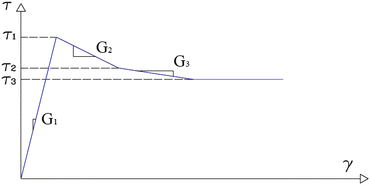

  

  Parameters of strain-softening soil model

• Shear modulus of the loading/unloading response, G₁, together with the shear moduli of the strain softening branches, G₂ and G₃ (Fig. 18.1); alternatively, the shear strains corresponding to the three shear stresses in Fig. 18.1.

Damping in the loading/unloading cycles is simulated by the Rayleigh damping (e.g. Chopra, 2001) which is defined as C = α M + β K where M and K are the mass and stiffness matrices.

A model with N soil layers over a half space contains N + 1 degrees of freedom corresponding to the displacements at the soil interfaces. The differential equation of motion of this model is given by:

$$ \boldsymbol{M}\kern0.15em {\ddot{\boldsymbol{U}}}+\boldsymbol{C}\kern0.15em {\dot{\boldsymbol{U}}}+\boldsymbol{K}\kern0.15em {\dot{\boldsymbol{U}}}=-\boldsymbol{M}\left\{\boldsymbol{I}\right\}\ {\ddot{u}}_g(t) $$

(18.1)

where M, K and C are the mass, stiffness and damping matrices of the system, U is the vector of displacements at layer interfaces relative to the base, and ü _g (t) is the earthquake acceleration on the half-space outcrop. The symbol {I} denotes a vector of N + 1 unit values. The equations of motion were solved by the constant acceleration method which is an implicit and unconditionally stable integration algorithm (e.g. Chopra 2001).

18.3.2 Model Parameters

The analyses included two different clay types, sensitive and ordinary clays. As shown in Fig. 18.1, a strain-softening soil model was used for the sensitive clay. The normalized small-strain shear modulus (G_max/S_u ^DSS) for clay was established as a function of plasticity index (I_p) using (18.2) based on the lab test data presented by Andersen (2004). The soil parameters used in the analyses are summarized in Table 18.2.

Table 18.2 Model parameters for sensitive clays and clays

$$ \frac{G_{max}}{s_u^{DSS}}=325+\frac{55}{{\left(\frac{I_p}{100}\right)}^2} $$

(18.2)

It is admitted that the results of this study (especially those for the sensitive clay) are dependent on the selected soil parameters. Nevertheless, it is believed that these results provide a step in the right direction in the development of more reliable predictive equations.

A normally consolidated soil profile with a normalized direct simple shear strength value s_u ^DSS/ σ’_v = 0.21 (with σ’_v being the effective vertical stress) was used for the analyses. To account for the increased strength under dynamic loading, a strain rate factor of 1.4 was applied to the static shear strength (Lunne and Andersen 2007). To capture the variation in the slope angle and soil profiles, the analyses were conducted for slope angles of 3°, 6°, 9°, and 12° and for soil profile depths of 40 m, 70 m, and 100 m. The numerical analyses were carried out for five earthquake strong motions records using PGA levels ranging from 0.05 g to 0.40 g (next section). Totally, 315 QUIVER analyses were performed for sensitive clay slopes and 515 analyses were conducted for clay slopes.

18.4 Selection and Scaling of Acceleration Time Histories

The acceleration response spectrum used in Norway for rock (ground type A according to Eurocode 8 terminology) was used as the target spectrum. The spectrum is shown in Fig. 18.2 for PGA = 0.05 g. The spectrum follows the standard parameterized form in Eurocode 8. Pacific Earthquake Engineering Research (PEER) Ground Motion Database Web Application (PGMD) was used for the selection of the best matching earthquake strong motion records. PGMD allows the user to select recordings for which the geometric mean of the two horizontal components provides a good match to the target spectrum. The quantitative measure of the ‘good match’ of the motion with respect to the target spectrum is evaluated by Mean Squared Error (MSE) of the difference between the spectral accelerations of the record and the target spectrum. Scale factors are applied to reduce the MSE over the period range of interest. The scaling factor is applied to the geometric mean of two horizontal components so the same scale factor is applied over the two components for the same strong motion data.

Fig. 18.2

Target acceleration spectrum corresponding to PGA = 0.05 g and response spectra of scaled acceleration time histories

Five horizontal components of recorded earthquake strong motions from the PEER Center strong motion database (PEER 2011) were selected as seed motions, and they were scaled to the horizontal target spectrum. Table 18.3 summarizes the relevant parameters of the selected seed motions. The scaling factors used for these motions are also presented in Table 18.3. The response spectra of the scaled time histories and the target spectrum are plotted in Fig. 18.2.

Table 18.3 Main parameters of selected recorded motions

18.5 Development of Predictive Models

The two parameters, PGA and yield acceleration, have commonly been used in the earlier predictive models based on the sliding-block concept. These parameters give measures of the driving force and resistance, respectively. While PGA on bedrock has a clear role in sliding block models, it loses its significance in realistic soil profiles. A more representative parameter for the driving force is the peak acceleration on the ground surface that relates closely to the destabilizing force on the slope mass. The yield acceleration is closely related to the factor of safety, FS, and hence was replaced by this parameter in the present study. The advantage of using FS in the predictive equations is that one could readily extend the equations derived from the 1D analyses to more general 2D and 3D geometries. A limited number of 2D seismic slope analyses are used in this paper to test the validity of this idea. In applying the presented predictive equations, the value of FS should be computed by using the peak shear strength applicable to earthquake loading, for example after it is increased to account for the rate effect.

The existing predictive models give only estimates of the slope displacements. The underlying assumption is that if the computed displacement is larger than a threshold value (typically in the range 5-15 cm), the slope is considered to fail. As pointed out earlier, permanent shear strain is a more robust indicator of slope stability as compared to sliding displacement. Laboratory test data could then be used to establish the threshold shear strain for initiation of soil failure. While in clay the threshold can be as large as 15 %, for sensitive and quick clay the value is much smaller due to the possibility of undrained creep failure (e.g. Andersen 2009).

18.5.1 Permanent Slope Displacement in Sensitive Clay

Figure 18.3a, b show the computed permanent displacements as a function of the computed peak acceleration on the ground surface with different labels for slope angles and for earthquake strong motion records, respectively. Figure 18.4a, b show the histograms of the computed displacements and the peak acceleration on the ground surface from 315 seismic response analyses for sensitive clay slopes.

Fig. 18.3

Permanent displacement versus peak acceleration on ground surface for sensitive clay with labels (a) for slopes angles, and (b) for selected acceleration-time histories (GM stands for Ground Motion)

Fig. 18.4

Histograms of (a) permanent displacement, and (b) peak acceleration on ground surface in sensitive clay

Equation 18.3 shows the functional form of the predictive model. In this equation, a _max is the peak acceleration on the ground surface in g, and D is the permanent displacement in cm. The standard deviation (σ_lnD) for the best fit predictive model is 1.15. Figure 18.5 shows the prediction of the model for different slope angles.

Fig. 18.5

Displacement predictions of model for sensitive clay slopes for (a) all displacement values, and (b) zoomed-in region for D < 15 cm

$$ \ln D=5.89+2.65 \ln \left({a}_{max}\right)-0.51 FS-0.4\left( FS-3.11\right)\left( \ln \left({a}_{max}\right)+1.4\right) $$

(18.3)

18.5.2 Permanent Slope Displacement in Clay

Figure 18.6a, b show the computed permanent displacements as function of the computed peak acceleration on the ground surface with different labels for slope angles and for earthquake strong motion records, respectively. Figures 18.6a and 18.7b show the histograms of the computed permanent displacements and the peak acceleration on ground surface from 515 seismic response analyses for clay slopes.

Fig. 18.6

Permanent displacement versus peak acceleration on ground surface in clay slopes with labels (a) for slope angles, and (b) for selected acceleration time histories (GM stands for Ground Motion)

Fig. 18.7

Histograms of (a) permanent displacement, and (b) peak acceleration on ground surface in clay slopes

Equation 18.4 shows the functional form of the predictive model. The standard deviation (σ_lnD) for the best fit predictive model is 0.97. Figure 18.8 displays the prediction of the model for different slope angles.

Fig. 18.8

Displacement predictions of model for clay slopes for (a) all displacement levels, and (b) zoomed-in region for D < 15 cm

$$ \ln D=5.65+2.57 \ln \left({a}_{max}\right)-0.50 FS-0.3\left( FS-2.96\right)\left( \ln \left({a}_{max}\right)+1.3\right) $$

(18.4)

18.5.3 Permanent Shear Strain in Sensitive Clay

Figure 18.9a, b display the computed permanent shear strains as function of the computed peak acceleration on the ground surface with different labels for slope angles and for earthquake strong motion records, respectively. Figure 18.10a, b present the histograms of the permanent strains and the peak acceleration on ground surface for 315 seismic slope response analyses for sensitive clay.

Fig. 18.9

Permanent shear strain versus peak acceleration on ground surface for sensitive clay, with labels (a) for slopes angles, and (b) for selected acceleration time histories

Fig. 18.10

Histograms of (a) permanent shear strain, and (b) peak acceleration on ground surface for sensitive clay

Equation 18.5 expresses the functional form of the predictive model. The standard deviation (σ_lnS) for the best fit predictive model is 1.19. In this equation, S is the permanent shear strain in percent, and a _max is the peak acceleration (in g) on the ground surface. Figure 18.11 shows the prediction of the model for different slope angles.

Fig. 18.11

Shear strain predictions of model for sensitive clay for (a) all strain levels, and (b) zoomed-in region for S < 10 %

$$ \ln S=5.75-0.52 \,\, FS+2.77 \ln \left({a}_{max}\right)+0.076 \,\, FS \,\, \ln \left({a}_{\max}\right) $$

(18.5)

18.5.4 Permanent Shear Strain in Clay

Figure 18.12a, b present the computed permanent shear strains as function of the computed peak acceleration on the ground surface with different labels for slope angles and for earthquake strong motion records. Figure 18.13a, b show the histograms of the permanent strain and the peak acceleration on ground surface out of 515 seismic slope response analyses for clay slopes.

Fig. 18.12

Permanent shear strain versus peak acceleration on ground surface with labels for clay slopes (a) for slope angles, and (b) for selected acceleration time histories

Fig. 18.13

Histograms of (a) permanent shear strain and (b) peak acceleration on ground surface in clay slopes

Equation 18.6 gives the functional form of the predictive model. The standard deviation (σ_lnS) for the best fit predictive model is 0.92. Figure 18.14 shows the prediction of the model for different slope angles.

Fig. 18.14

Permanent shear strain predictions of model for clay slopes for (a) all strains levels, and (b) zoomed-in region for S < 10 %

$$ \ln S=4.15-0.30 \,\, FS+2.06 \,\, \ln \left({a}_{max}\right)+0.16 \,\,FS \,\, \ln \left({a}_{\max}\right) $$

(18.6)

18.5.5 Comparisons of Displacement and Strain Predictions for Clay and Sensitive Clay

Figure 18.15 presents a comparison of the displacement predictions for clay and sensitive clay. Figure 18.16 shows a comparison of the permanent shear strain predictions for ordinary and sensitive clays. As expected, for the same slope geometry and similar earthquake loading, the displacements and shear strains are larger for the sensitive clay.

Fig. 18.15

Displacement predictions for clay and sensitive clay

Fig. 18.16

Shear strain predictions for clay and sensitive clay

18.6 Comparison with Other Predictive Models for Displacement

Figure 18.17 presents a comparison of several predictive models (namely, Watson-Lamprey and Abrahamson 2006; Bray and Travasarou 2007, the Jibson 2007 k _y /PGA model, the Rathje and Saygili 2009 scalar (PGA, M) model and the Saygili and Rathje 2008 vector (PGA, PGV) model) for a deterministic earthquake scenario of M _w  = 7.5 and R = 5 km for a shallow, rigid sliding mass, and rock site conditions (V_s30 > 760 m/s). The predicted ground motion parameters for each scenario are listed in the figure. The values of PGA and Sa _T=1s are from Boore and Atkinson (2008), I _a is from Travasarou et al. (2003), T _m is from Rathje et al. (2004), and D _5–95 is from Abrahamson and Silva (1997). Even though these models were developed using large datasets and rigorous regression techniques, there is more than a magnitude difference in the final predictions. The Bray et al. (1998) model predicts the largest displacement, the Watson-Lamprey and Abrahamson (2006) model predicts the smallest, and the other models fall in between. As shown in the figure, the displacement predictions of the proposed model fall into the low estimate bound for less stable slopes (e.g. k_y = 0.05–0.10 g) and into the high estimate bound for more stable slopes (k_y = 0.20–0.25 g). The proposed model uses the maximum acceleration on the ground surface whereas the other models use PGA in the equations. It should be noted that Jibson (2007), Bray and Travasarou (2007), Rathje and Saygili (2009) and the proposed model each use only one ground motion parameter (PGA), while Saygili and Rathje (2008) and Bray et. al. (1998) use two ground motion parameters, and the Watson-Lamprey and Abrahamson (2006) model uses four parameters (PGA, A _RMS , Sa _T=1s , and Dur _ky ).

Fig. 18.17

Comparisons of predictive models for sliding displacement for a deterministic scenario of M_w = 7.5 and R = 5 km

18.7 Comparison of Displacement Predictions with 2D FEM Results

The predictive models were developed from a database of numerically computed response parameters using 1D earthquake analyses. The factor of safety, FS, was used in the predictive equations with the intention that these equations could be applied to more general soil types and slope geometries. A natural step along this line is to test the performance of the developed models in a two-dimensional geometry. To this end, a number of simple 2D slope models with normally-consolidated clay were constructed and were excited by earthquake at their bases. The permanent displacements and permanent shear strains in these slopes were computed at the end of the shaking and were compared with the predictions from the developed equations. The analyses were carried out with the FE software Plaxis.

Figure 18.18 displays part of the slope model used in the analyses together with its FE mesh. The model is 75 m deep on the downslope side and 110 m deep on the upslope side. The slope was placed in two series of analyses such that their factors of safety, SF, were 1.2 and 1.5. Because the peak accelerations and permanent displacements vary on the ground surface, seven monitoring points (points B to H, as shown in Fig. 18.18), were placed on the ground surface. The slopes were excited by acceleration time histories with PGA varying from 0.05 g to 0.40 g on the bedrock (base of the model, point A in Fig. 18.18). The values of the peak accelerations and permanent displacements at the monitoring points were determined from the FE analyses and were averaged. For the permanent shear strain, the maximum value was determined from each analyses.

Fig. 18.18

Two-dimensional FE model, mesh detail and monitoring points on ground surface

Figure 18.19a, b present typical results of the FE analyses for the case FS = 1.2 due to an earthquake with PGA = 0.4 g. Figure 18.19a displays the contours of permanent slope displacements. The displacement values range from 0.0 to 1.3 m. Figure 18.19b displays the contours of the permanent shear strains. The values range from 0.0 to about 10 % at the toe of the slope.

Fig. 18.19

Results of 2D FE analyses for slope with FS = 1.2 and PGA = 0.4 g: (a) permanent horizontal displacements with maximum value about 1.3 m, (b) permanent shear strains with maximum value 10 %

Figure 18.20 compares the results of the 2D FE analyses with the predictive models developed in this paper. The figures show the comparison of both the permanent displacements and permanent shear strains. For the former parameter, both the average 2D results and the maximum values are plotted. For the latter parameter, the maximum permanent strains from the 2D model are plotted together double the strains. The reason for this is that the shear strain is more sensitive to the FE mesh size, and there is a tendency that the maximum strain increases, as the mesh is refined. The results in both cases show fairly good agreement with those from the predictive models.

Fig. 18.20

Results from 2D FEM for FS = 1.2 versus best fit predictions, (a) permanent displacements, (b) permanent shear strains

Figure 18.21 presents similar comparisons for the case FS = 1.5. While comparison of the displacements by the FE model and predictive model is satisfactory, the predictive model for shear strain tends to overly estimate the shear strains. This is a typical effect of 2D geometry which represents a conservative situation compared to a 1D idealization. As the size of the slope increases, this effect is diminished, and the 2D results tend more to the 1D results as captured by the predictive models developed in this paper.

Fig. 18.21

Results from 2D FEM for FS = 1.5 versus best fit predictions, (a) permanent displacements, (b) permanent shear strains

References

Abrahamson NA, Silva W (1997) Empirical response spectral attenuation relations for shallow crustal earthquakes. Seismol Res Lett 68:94–127
Andersen KH (2004) Cyclic clay data for foundation design of structures subjected to wave loading. In: Proceedings of the international conference of cyclic behaviour of soils and liquefaction phenomena. A. A. Balkema Publishers, Bochum, pp 371–387
Andersen KH (2009) Bearing capacity under cyclic loading — offshore, along the coast, and on land. The 21st Bjerrum Lecture presented in Oslo, 23 November 2007. Can Geotech J 46(5):513–535
Biscontin G, Pestana JM, Nadim F (2004) Seismic triggering of submarine slides in soft cohesive soil deposits. Mar Geol 203(3 & 4):341–354
Boore DM, Atkinson GM (2008) Ground-motion prediction equations for the average horizontal component of PGA, PGV and 5 %-damped PSA at spectral periods between 0.01 s and 10.0 s. Earthq Spectra EERI 24(1):99–138
Bray JD, Travasarou T (2007) Simplified procedure for estimating earthquake-induced deviatoric slope displacements. J Geotech Geoenviron Eng ASCE 133(4):381–392
Bray JD, Rathje EM, Augello AJ, Merry SM (1998) Simplified seismic design procedure for lined solid-waste landfills. Geosynthet Int 5(1–2):203–235
Chopra AK (2001) Dynamics of structures. Theory and applications to earthquake engineering, 2nd edn. Prentice Hall, Englewood Cliffs
Jibson RW (2007) Regression models for estimating coseismic landslide displacement. Eng Geol 91:209–218
Johansson J, Lovolt F, Andersen KH, Madshus C, Aabøe R (2013) Impact of blast vibrations on the release of quick clay slides. In: Proceedings of 18th international conference on soil mechanics and geotechnical engineering, ICSMGE, Paris
Kaynia AM (2011) QUIVER_slope – numerical code for one-dimensional seismic response of slopes with strain softening behaviour. NGI report 20071851-00-79-R, 8 June 2012
Lunne T, Andersen KH (2007) Soft clay shear strength parameters for deepwater geotechnical design. In: Proceedings 6th international conference, society for underwater technology, offshore site investigation and geotechnics, London, pp 151–176
Nadim F, Kalsnes B (1997) Evaluation of clay strength for seismic slope stability analysis. In: Proceedings XIV ICSMFE, Hamburg, vol 1, pp 377–379, 6–12 Sept 1997
Newmark NM (1965) Effects of earthquakes on dams and embankments. Geotechnique 15(2):139–160
PEER – PGMD (2011) Website – http://peer.berkeley.edu/peer_ground_motion_database/
Rathje EM, Bray JD (1999) An examination of simplified earthquake-induced displacement procedures for earth structures. Can Geotech J 36(1):72–87
Rathje EM, Bray JD (2000) Nonlinear coupled seismic sliding analysis of earth structures. J Geotech Geoenviron Eng 126(11):1002–1014
Rathje EM, Saygili G (2009) Probabilistic assessment of earthquake-induced sliding displacements of natural slopes. Bull N Z Soc Earthq Eng 42:18–27
Rathje EM, Faraj F, Russell S, Bray JD (2004) Empirical relationships for frequency content parameters of earthquake ground motions. Earthq Spectra 20(1):119–144
Saygili G, Rathje EM (2008) Empirical predictive models for earthquake-induced sliding displacements of slopes. J Geotech Geoenviron Eng ASCE 134(6):790–803
Travasarou T, Bray JD, Abrahamson NA (2003) Empirical attenuation relationship for Arias intensity. Earthq Eng Struct Dyn 32(7):1133–1155
Watson-Lamprey J, Abrahamson N (2006) Selection of ground motion time series and limits on scaling. Soil Dyn Earthq Eng 26(5):477–482
Author information
Authors and Affiliations
Corresponding author
Editor information
Editors and Affiliations
Rights and permissions
This chapter is published under an open access license. Please check the 'Copyright Information' section either on this page or in the PDF for details of this license and what re-use is permitted. If your intended use exceeds what is permitted by the license or if you are unable to locate the licence and re-use information, please contact the Rights and Permissions team.
Copyright information
© 2014 The Author(s)
About this chapter
Cite this chapter
Kaynia, A.M., Saygili, G. (2014). Predictive Models for Earthquake Response of Clay and Sensitive Clay Slopes. In: Ansal, A. (eds) Perspectives on European Earthquake Engineering and Seismology. Geotechnical, Geological and Earthquake Engineering, vol 34. Springer, Cham. https://doi.org/10.1007/978-3-319-07118-3_18
Download citation
DOI: https://doi.org/10.1007/978-3-319-07118-3_18
Published:
Publisher Name: Springer, Cham
Print ISBN: 978-3-319-07117-6
Online ISBN: 978-3-319-07118-3
eBook Packages: Earth and Environmental ScienceEarth and Environmental Science (R0)