Groundwater

Abstract

An aquifer is an underground body of water perched on top of bedrock or other impermeable layer. Most usable freshwater storage is within aquifers (Table 10.1). The residence time of groundwater can vary from days to millennia (Fig. 10.1). Groundwater’s often long period of water exchange (Table 10.1) makes it useful as a stable source of water but also leads to its susceptibility to long term degradation by aquifer contamination. Groundwater supplies approximately 40 % of the water used by irrigated agriculture. Wells are drilled into high conductivity layers in geologic formations. Sand and gravel aquifers are the primary source of groundwater for irrigation. Measurement of the piezometric gradient and aquifer hydraulic conductivity enables hydrologists to calculate aquifer flow velocity and direction. The product of aquifer thickness and hydraulic conductivity is the transmissivity. The Thiem equation calculates aquifer transmissivity in confined aquifers based on steady-state pumping in a pumping well and draw down (decline in water table) in an observation well. The steady-state unconfined aquifer equation adds aquifer thickness to the equation. The Theis equation evaluates transient drawdown in an observation well.

Questions

• 1. What are the five major types of aquifers?

• 2. Describe four different types of aquifers commonly used for irrigation and give an example of each.

• 3. Draw a confined and unconfined aquifer.

• 4. Discuss groundwater recharge and discharge components for a basin

• 5. Discuss the impact of overpumping on stream flow in arid climates.

• 6. Discuss the natural condition and impact of man on the Ogallala aquifer.

• 7. Discuss the impact of irrigation on water table elevation and salinization.

• 8. Calculate the porosity, storativity, specific yield, and specific retention for an aquifer that has 40 % water below the water table, and yield of 1.2 m of water for every 5 m drop in water table elevation.

• 9. A coarse sand aquifer has a water table slope of 1 m/100 m. Evaluate at the upper and lower limits of coarse sand hydraulic conductivity. What is the Darcy velocity of the water in the aquifer? The cross sectional area of the aquifer is 100 m x 1,000 m. What is the volume of water flow in 1 year? Convert water volume to acre-ft. How many acres of cotton could be irrigated with this volume per year? Also calculate for a silt aquifer with a hydraulic conductivity at the lower end of silt conductivities.

• 10. Find the hydraulic gradient and the direction of flow with the East axis (x-axis) as zero degrees for the following three wells. Show your work (work it by hand), and check your work with the Groundwater program.

  	East	North	Elevation
  Well 1	50	600	104
  Well 2	400	250	105
  Well 3	200	50	108

• 11. If the aquifer in question 10 is a coarse sand aquifer with hydraulic conductivity equal to 100 m/day and porosity of 0.40 calculate the Darcy velocity and the velocity that a contaminant plume would travel through the aquifer.

• 12. What is the reason that aquifer pollution is much more difficult to correct than surface water pollution?

• 13. What are the primary pollutants from agriculture that have contributed to aquifer pollution?

• 14. What often happens to shallow aquifers when irrigation is introduced to a region?

• 15. Find the transmissivity and conductivity of confined aquifer in which the flow rate to a well is 400 gpm, and observation wells at distances of 100- and 200-m from the pumping well have depths to the water table of 100-m and 98-m, respectively. The upper surface of the aquifer is 140 m below ground and the aquifer is 40 m thick. Check your calculations with the Confined aquifer worksheet.

• 16. Find the conductivity and transmissivity in an unconfined aquifer in which the flow rate to a well is 400 gpm, and observation wells at distances of 100- and 200-m from the pumping well have depths to the water table of 100-m and 98-m, respectively. The lower boundary of the aquifer (upper surface of aquitard) is 150 m below the ground.

• 17. Calculate the transmissivity and storativity of a confined aquifer. The following drawdown data was collected from an observation well 100 m from the pumping well. The well flow rate was 2,000 m³/day.

  Time after initiation of pumping	Drawdown s (m)
  1 min	0.44
  2 min	0.55
  4 min	0.66
  8 min	0.77
  0.01 day	0.86
  0.02 day	0.97
  0.04 day	1.08
  0.08 day	1.19
  0.16 day	1.30
  0.32 day	1.41
  0.64 day	1.52
  1 day	1.59

• 18. For the aquifer in question 17, calculate the drawdown in the well for a series of points between 1 hr and 1 week. The well diameter is 50 cm (use r = 0.25 m in the Theis s vs. t worksheet). The pump flow rate is 3,000 m³/day.

• 19. The well described in questions 17 and 18 has a maximum acceptable drawdown of 20 m inside the well. The pressure loss in the casing is flow rate (m³/day)/4,600. Calculate the maximum allowable pump flow rate and the drawdown at 80 %, 60 %, 40 %, and 20 % of maximum. Plot the drawdown vs. flow rate curve. What is the shape of the curve? Convert the maximum flow rate to units of GPM and report whether this well would be considered a good well. Assume that the drawdown after 7 days is the steady state drawdown.

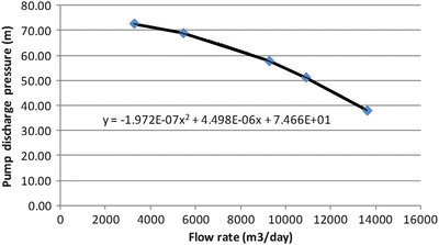
• 20. The static water table in the aquifer described in questions 17–19 is 40 m below the ground surface. The pump in the well has a pump curve as shown below. The pump has an open discharge 0.5 m above the ground surface, and the sum of minor losses (K) = 3.9 (including velocity head losses at the discharge). The pump hangs on a 12 inch pipe (Schedule 40) at an elevation 80 m below the ground surface, and there is a 2 m section of pipe above the ground surface (total 82 m pipe). The pipe has a Hazen Williams C = 100. Include the minor losses. Calculate the discharge flow rate.

  

• 21. What are the two types of groundwater pollution? Which comes from field agriculture?