On Structure-Preserving Cryptography and Lattices

Abstract

The Groth-Sahai proof system is a highly efficient pairing-based proof system for a specific class of group-based languages. Cryptographic primitives that are compatible with these languages (such that we can express, e.g., that a ciphertext contains a valid signature for a given message) are called “structure-preserving”. The combination of structure-preserving primitives with Groth-Sahai proofs allows to prove complex statements that involve encryptions and signatures, and has proved useful in a variety of applications. However, so far, the concept of structure-preserving cryptography has been confined to the pairing setting.

In this work, we propose the first framework for structure-preserving cryptography in the lattice setting. Concretely, we

• define “structure-preserving sets” as an abstraction of (typically noisy) lattice-based languages,

• formalize a notion of generalized structure-preserving encryption and signature schemes (capturing a number of existing lattice-based encryption and signature schemes),

• construct a compatible zero-knowledge argument system that allows to argue about lattice-based structure-preserving primitives,

• offer a lattice-based construction of verifiably encrypted signatures in our framework.

Along the way, we also discover a new and efficient strongly secure lattice-based signature scheme. This scheme combines Rückert’s lattice-based signature scheme with the lattice delegation strategy of Agrawal et al., which yields more compact and efficient signatures.

We hope that our framework provides a first step towards a modular and versatile treatment of cryptographic primitives in the lattice setting.

B. Ursu—Author based in Zurich, Switzerland and work carried out during the author’s time at ETH Zurich.

1 Introduction

Structure-Preserving Cryptography. Groth-Sahai (GS) proofs [34] are practical non-interactive zero-knowledge (NIZK) proof systems for a very general class of group-based languages. Essentially, GS proofs allow to argue in zero-knowledge about the satisfiability of systems of equations over groups that may involve exponentiation, of course group operations, and even pairing operations. When used in conjunction with “suitably algebraic” group-based cryptographic primitives (like encryption or signature schemes), GS proofs allow to efficiently prove complex statements like “This ciphertext contains an electronic passport for John Smith that is certified by a government authority.”¹ In comparison to a generic approach (with, say, a generic NIZK system for NP [26]), such a “native” approach is significantly more practical.

“Suitably algebraic” cryptographic primitives are called structure-preserving [2, 32] (or, in a slightly different formulation, automorphic [28]). Numerous examples of structure-preserving signature (e.g., [1,2,3, 19, 20, 33]) and public-key encryption schemes (e.g., [15, 23, 25, 37]), as well as other primitives (e.g., [12, 50]) are known, based on different computational assumptions, and having different efficiency and security features.

All of these building blocks can be combined, and GS proofs can be used to argue about such combinations efficiently. However, so far, the paradigm of structure-preserving relies on a particular algebraic setting (of pairing-friendly cyclic groups), and it is unclear whether a similar modular combination of cryptographic primitives is also possible over other domains.²

This Work: Structure-Preserving Cryptography over Lattices. In this work, we initiate the study of structure-preserving cryptography over lattices. We put forward suitable definitions of structure-preserving signature and encryption schemes, and present a suitable NIZK system for proving statements about combinations of these primitives. Hence, in short, our core contributions are

• a suitable definition of lattice-based structure-preserving cryptographic primitives (including the modeling of a number of existing signature and encryption schemes according to this definition),

• a suitable zero-knowledge argument system that allows to show statements about lattice-based structure-preserving primitives,

• as an application (and to demonstrate the usefulness of our approach), a modular lattice-based protocol for verifiably encrypted signatures.

As we will explain, our notion of lattice-based structure-preserving primitives is not quite as universal as in the GS setting. This allows us to model a large class of primitives, but also asks for some degree of compatibility among the used primitives. We still believe that our abstract framework is a step towards plug-and-play lattice-based cryptography. Indeed, one benefit of our approach is modularity: It is true that the security analysis for each lattice-based component (i.e., signature or encryption scheme) needs to keep track of noise growth and failure probabilities. However, due to our interface, this analysis needs to be done only once per component, not once for every possible combination of components.

Contribution 1: A Definition of Lattice-Based Structure-Preserving Primitives. First, we cannot use or easily adapt existing (group-based) definitions of structure-preserving primitives: with computations over lattices, there is no equivalent of “exponentiation” or “pairing”. Besides, typically lattice-based ciphertexts or signatures often feature a “noise term”, which may grow with operations on these values. Once the noise term becomes too large, decryption or verification becomes unreliable. Hence, operations on these values are limited in a quantitative way, and this limitation should be reflected in a definition of structure-preserving cryptography.

Since lattice-based cryptographic constructions usually work over the ring $\mathbb {Z}_q$ (for a suitable integer $q$), it is tempting to call the solutions to arbitrary systems of linear equations over $\mathbb {Z}_q$, possibly with boundaries on norms (to accommodate noise terms), structure-preserving. Unfortunately, we do not know how to instantiate a proof system for such general sets in the standard model.³

So instead of trying to match the group-based definition, we start from scratch with a relatively simple definition of “structure-preserving sets” modelling exactly the noise terms of lattice-based cryptography. We present a standard-model non-interactive proof system for these sets, and aim to interpret signatures and ciphertexts (or, rather, the randomness of ciphertexts) as structure-preserving sets. To express more powerful statements in terms of structure-preserving sets, we additionally require our structure-preserving signature and encryption schemes to allow for suitable homomorphic operations (that, e.g., allow to verify a signature inside an encryption scheme).

Fortunately, we discover that several existing signature and encryption schemes satisfy our definitions. Examples include Regev encryption [45] and its dual variant [30], the GSW leveled homomorphic encryption scheme [31], and the signature schemes of Boyen [14] and Rückert [46].⁴

At this point, the mentioned required compatibility among used primitives is crucial: we unfortunately cannot combine arbitrary lattice-based structure-preserving encryption and signature schemes. Essentially, we require that the encryption scheme allows to homomorphically verify an encrypted signature. This allows to combine, e.g., the GSW FHE scheme with all of the mentioned signature schemes; alternatively, we can combine any additively homomorphic scheme (such as Regev’s scheme or its dual variant) with Rückert’s scheme or its mentioned new and more compact variant, but not with Boyen’s scheme.

Contribution 2: A Compatible NIZK Argument System. To allow arguing about combinations of encryption and signature schemes, we also introduce an analogue of GS proofs. In our case, we use the LWE-based NIZK system of Libert et al. [36] as a basis. This proof system is based upon a $\varSigma$-protocol [21] for proving that an LWE encryption contains a certain value. (That $\varSigma$-protocol is later converted to a NIZK system by applying the Fiat-Shamir transform [27] in the standard model, with a correlation-intractable hash function). To suit our needs, however, we need to generalize this proof system to structure-preserving sets (i.e., to statements that are valid “up to noise”). This requires a more careful analysis, and in particular a liberal use of rejection sampling [38].

We should emphasize that we are interested in a standard-model proof system. Indeed, while our application does not require this, we would like to be able to argue about encrypted proofs (and thus achieve the “nestable” property of Groth-Sahai proofs). If proof verification involves random oracle queries, this is not possible transparently. We should note, however, that our proof system supports only linear languages, while its verification itself is not linear. Hence, nesting proofs of our proof system is only possible when using leveled homomorphic encryption schemes (that allow to verify even a nonlinear encrypted proof through homomorphic evaluation). We leave open the construction of a lattice-based proof system for a language that includes its own verification.

Contribution 3: Lattice-Based Verifiably Encrypted Signatures. Finally, we demonstrate the usefulness of our approach using the setting of verifiably encrypted signatures [7, 13, 29, 47]. Concretely, we show how to combine lattice-based structure-preserving signature and an encryption schemes to obtain a scheme that allows to prove that a given ciphertext contains an encryption of a valid signature for given (publicly known) message. While generic constructions (e.g., using lattice-based zero-knowledge for NP [43]) for this task are possible, and very efficient techniques for related problems exist in the random oracle world [24, 42], it appears that our protocol is the first non-generic (i.e., at least somewhat efficient) lattice-based verifiably encrypted signature scheme in the standard model.

More Related Work. As already mentioned, there is a very successful line of work [8, 24, 40, 41] that aims at practical (non-interactive) zero-knowledge proofs from lattices in the random oracle model. The supported languages are very general and include typical “noisy linear” languages, as crucial for many lattice-based schemes. Conceptually, these schemes are commit-and-prove schemes, much like Groth-Sahai proofs.

On the other hand, the use of random oracles appears inherent. For instance, the scheme from [40] is obtained by using the Fiat-Shamir transform on a suitable $\varSigma$-protocol. Unlike in our setting, these $\varSigma$-protocols do not appear to satisfy the requirements for the use of correlation-intractable hash functions as replacements for random oracles. Still, when one is not interested in nesting proofs (and if one accepts random oracles), then these protocols appear to be excellent replacements for our proof system.

1.1 Technical Overview

We now take a closer look at our framework. Our first step will be to define structure-preserving sets, an abstraction of “noise terms” that are omnipresent in lattice-based cryptography.

Structure-Preserving Sets. We call a set $S\subseteq \mathbb {Z}_q^d$ structure-preserving if there is a (“noise”) distribution $\mathcal {D}$ such that

• $\mathcal {D}$ “smudges” elements from $S$ in the sense that for any $\mathbf {{s}},\mathbf {{s}}'\in S$ and $\mathbf {{d}}\leftarrow \mathcal {D}$, the values $\mathbf {{s}}+\mathbf {{d}}$ and $\mathbf {{s}}'+\mathbf {{d}}$ are statistically close.⁵

• Smudging with $\mathcal {D}$ preserves (non-)membership in $S$, in the sense that for $\overline{S}=\mathbb {Z}_q^d\setminus S$, we have that $S+\mathop {\textrm{supp}}\limits (\mathcal {D})$ and $\overline{S}+\mathop {\textrm{supp}}\limits (\mathcal {D})$ are disjoint.⁶ This condition guarantees that the smudging process is non-trivial.

The set of short-norm vectors is structure-preserving according to (the non-oversimplified version of) this definition. But structure-preserving sets also cover more complex cases, such as the set of vectors close to a given vector, (the union of) intervals, or the cartesian product of structure-preserving sets. In essence, we only require that a structure-preserving set is “non-trivially smudgeable”.

Jumping ahead, structure-preserving sets will be used to model, e.g., the “raw” (i.e., un-rounded) verification output of signature schemes. This verification output only encodes a bit (the verification verdict), but may need to be smudged for further processing to avoid leakage about the signature. In fact, we now proceed to (informally) define structure-preserving signature and encryption schemes.

Structure-Preserving Signatures. A (lattice-based) signature scheme is called structure-preserving for a family $\mathcal {F}$ of functions if each verification key $\textsf{vk}$ and message $\textsf{msg}$ defines an $f\in \mathcal {F}$ such that a given signature $\sigma$ is valid if and only if $f(\sigma )\in S$ for a (fixed) structure-preserving set $S$.⁷ We will be particularly interested in families $\mathcal {F}$ of linear functions, since such $\mathcal {F}$ will allow for (non-generic) zero-knowledge proofs. This is also the reason for the need to smudge $f$’s output: existing lattice-based signature schemes usually postprocess the result of a linear operation with a rounding step obtain the verification verdict bit. Instead of this rounding step, we require that $f(\sigma )\in S$.

We show that Rückert’s signature scheme [46] is structure-preserving for a linear $\mathcal {F}$, and that Boyen’s signature scheme [14] is structure-preserving for an $\mathcal {F}$ that contains linear functions and functions computed by low-depth Boolean circuits. Additionally, we present a more compact variant of Rückert’s scheme (that is also strongly secure and structure-preserving for a linear $\mathcal {F}$). This new scheme is retrieved by replacing the “Bonsai trees” lattice delegation method of [18] with the more compact lattice delegation strategy of [5].

Structure-Preserving Encryption. We say that a (lattice-based) encryption scheme is structure-preserving if ciphertexts are of the form

$$\begin{aligned} \textsf{ct}=\mathbf {{B}}\mathbf {{r}}+g(\textsf{msg}) \end{aligned}$$

for a matrix $\mathbf {{B}}\in \mathbb {Z}_q^{d\times r}$, $\mathbf {{r}}\in S$ for a structure-preserving set $S$, and an invertible and additively homomorphic “message encoding function” $g$.⁸ Intuitively, we require that $\mathbf {{r}}\in S$ to be able to argue about “valid encryptions” (for which the encrypted message is uniquely determined).

For our applications, it will also be beneficial if the scheme is $\mathcal {F}$-homomorphic, in the sense that $\textsf{ct}=\mathbf {{B}}\mathbf {{r}}+g(\textsf{msg})$ allows to efficiently compute $\textsf{ct}'=\mathbf {{B}}\mathbf {{r}}'+g(f(\textsf{msg}))$ for any $f\in \mathcal {F}$ (possibly at the price of a larger noise).

We observe that Regev’s encryption scheme [45], its dual variant [30], and the GSW leveled homomorphic encryption scheme [31] fit our framework (for linear functions, resp. low-depth circuits). While itself not technically involved, this provides a helpful uniform way to reason about these schemes.

A Zero-Knowledge Protocol for Encrypted Structure-Preserving Sets. Our last ingredient is a suitable (lattice-based, non-interactive) zero-knowledge proof system that allows to argue about structure-preserving primitives (and in particular structure-preserving sets). More concretely, we start with a $\varSigma$-protocol that shows that a given ciphertext (from an arbitrary structure-preserving encryption scheme) encrypts an element $\textsf{msg}\in S$ from a structure-preserving set $S$.

This $\varSigma$-protocol is derived from a $\varSigma$-protocol due to Libert et al. [36] for proving equality of encrypted messages (where the used encryption scheme is a variant [6] of Regev encryption). The basic protocol of [36] (following Schnorr’s blueprint [49]) proceeds as follows. Say that we want to show that a given ciphertext $\textsf{ct}$ is an encryption of $0$.⁹ The prover $P$ then starts by sending a fresh $0$-encryption $\textsf{ct}_0$ to the verifier $V$. Then $V$ chooses to either open $\textsf{ct}_0$ or $\textsf{ct}_0 + \textsf{ct}$ (by sending the random coins of that ciphertext).

Soundness follows from the fact that if $\textsf{ct}$ is not a $0$-encryption, then at least one of the two ciphertexts $\textsf{ct}_0$ and $\textsf{ct}_0+\textsf{ct}$ encrypts a nonzero value. (Of course, to obtain a negligible soundness error, the above protocol will have to be repeated). Zero-knowledge follows from the fact that if one knows in advance which ciphertext is opened, one can program $\textsf{ct}_0$ such that the to-be-opened ciphertext surely encrypts $0$.

In our setting, we want to prove that $\textsf{ct}$ encrypts some $\mathbf {{s}}\in S$ (without revealing $\mathbf {{s}}$). Since $S$ is a structure-preserving set, we can smudge $\mathbf {{s}}$ with a suitable smudging vector $\mathbf {{d}}\leftarrow \mathcal {D}$. When we set up $\textsf{ct}_0$ as an encryption of such a $\mathbf {{d}}$, we obtain that

• opening $\textsf{ct}_0$ reveals only a smudging value $\mathbf {{d}}$, and

• opening $\textsf{ct}_0+\textsf{ct}$ reveals a smudged value $\mathbf {{s}}+\mathbf {{d}}$, which is (almost) statistically independent of $\mathbf {{s}}$.

Hence, using a similar strategy as in [36], we obtain zero-knowledge. Moreover, since smudging preserves (non-)membership in $S$, we obtain soundness (after sufficiently many repetitions). The actual proof is more involved than this overview, of course, largely because of the already mentioned rejection sampling necessary for statistical closeness.

We only briefly mention that our protocol is compatible with recent standard-model techniques [17, 43] to transform $\varSigma$-protocols in the lattice setting into non-interactive zero-knowledge (NIZK) proofs. We use a sophisticated variant [36] of this approach¹⁰ that even achieves unbounded simulation-soundness for specific classes of $\varSigma$-protocols. In the end, we obtain a NIZK argument system for encrypted structure-preserving sets.

From Structure-Preserving sets to Structure-Preserving Primitives. As an application (and to demonstrate the usefulness of our proof system), we construct a verifiably encrypted signature (VES [7, 13, 29, 47]) scheme. Intuitively, in a VES scheme, a dedicated signer hands out encrypted signatures (i.e., signatures generated using the signer’s secret key, and encrypted under the public key of a designated “adjudicator”). Such encrypted signatures also contain a NIZK proof of validity (i.e., of the fact that the given ciphertext really contains a valid signature for a given message). In case of a conflict, however, the adjudicator can extract (by decrypting) a “proper” (i.e., non-simulatable) signature from a given encrypted signature. VES schemes are useful, e.g., in contract signing applications [7, 13].

Using our framework, a lattice-based VES scheme can be obtained generically from a structure-preserving signature scheme, a structure-preserving encryption scheme with compatible message space (and such that it allows to homomorphically verify signatures), and our zero-knowledge proof system for (encrypted) structure-preserving sets. These primitives are combined in a straightforward way. Perhaps the most interesting part of this construction is the fact that it suffices to prove that an encrypted value comes from a structure-preserving set. Indeed, to prove that a given encryption contains a valid signature, we (a) first homomorphically verify that signature inside the encryption, and (b) then prove that the result corresponds to an “accept”. Recall that by our definition of structure-preserving signatures, this means proving membership in a structure-preserving set.

Our formal proof is similar to a proof for an existing VES scheme by Fuchsbauer [29] that uses pairing-based structure-preserving cryptography.

1.2 Roadmap

After recalling some notation and standard building blocks in Sect. 2, we present our definition of structure-preserving sets in Sect. 3. Building on this definition, we proceed with our notions of structure-preserving signatures (Sect. 4) and structure-preserving encryption schemes (Sect. 5). We identify and construct example schemes in Sect. 4.1 and 5.1 and more in the full version. Our $\varSigma$-protocol for (encrypted) structure-preserving sets appears in Sect. 6, followed by its conversion to a NIZK proof system in Section 7. The VES application follows in Section 8 where we also discuss its efficiency.

2 Preliminaries

2.1 Notation

A function f is negligible if for every polynomial $p(\cdot )$, there exists an $n_0 \in \mathbb {N}$ such that for every $n > n_0$ it holds that $f(n) < \frac{1}{p(n)}$. We write $\textsf{negl}$ to denote an arbitrary negligible function. Let X and Y be two probability distributions over a domain $\varOmega$. The statistical distance between X and Y is defined as $\varDelta (X,Y) :=\frac{1}{2} \sum _{\omega \in \varOmega } \vert \Pr [X=\omega ] - \Pr [Y = \omega ] \vert$. We say that two ensembles $\{ X_n\}_{n \in \mathbb {N}}$ and $\{ Y_n\}_{n \in \mathbb {N}}$ of distributions are statistically indistinguishable, denoted as $\{ X_n\}_{n \in \mathbb {N}} \approx _s\{ Y_n\}_{n \in \mathbb {N}}$, if $\varDelta (X_n,Y_n) = \textsf{negl}(n).$ We say that two ensembles $\{ X_n\}_{n \in \mathbb {N}}$ and $\{ Y_n\}_{n \in \mathbb {N}}$ of distributions are computationally indistinguishable, denoted as $\{ X_n\}_{n \in \mathbb {N}} \approx _c\{ Y_n\}_{n \in \mathbb {N}}$, if for every probabilistic polynomial time (PPT) adversary $\mathcal {A}$, we have $\vert \Pr [\mathcal {A}(X_n)=1]-\Pr [\mathcal {A}(Y_n)=1]\vert = \textsf{negl}(n).$

Let S be a finite set. Then by $x \leftarrow _{\textsc {r}}S$ we mean that x was sampled from the uniform distribution over S. For a probability distribution $\mathcal {D}$ on S we denoted the support by $\mathop {\textrm{supp}}\limits (\mathcal {D})\subseteq S$.

Let $\mathbf {{x}}\in \mathbb {R}^n$ be a column vector. The $x_i$, for $i \in \{1, \dots , n\}$ denotes the i-th coordinate of $\mathbf {{x}}$. The $\ell _2$-norm of $\mathbf {{x}}$ is defined as $\Vert \mathbf {{x}} \Vert :=\sqrt{\sum _{i=1}^n x_i^2}$. The $\ell _2$ norm of a matrix $\mathbf {{M}} \in \mathbb {R}^{n \times m}$ is defined as $\Vert \mathbf {{M}} \Vert = \sup _{\mathbf {{x}} \in \mathbb {R}^m, \mathbf {{x}} \ne 0}\frac{\Vert \mathbf {{M}} \mathbf {{x}}\Vert }{\Vert \mathbf {{x}} \Vert }$. We denote $\overline{\mathbf {{M}}}$ the Gram-Schmidt orthogonalization of the matrix $\mathbf {{M}}$.

For two sets $A, B \subseteq \mathbb {Z}_q^n$, we define the sets $A \setminus B, A + B, A - B \subseteq \mathbb {Z}_q^n$ as follows:

$$\begin{aligned} A \setminus B &:=\{ x \mid x \in A \ \wedge \ x \not \in B \}, \\ A + B &:=\{(a_1+b_1, \dots ,a_n+ b_n) \mid (a_1, \dots , a_n) \in A, (b_1, \dots , b_n) \in B \}, \\ A - B &:=\{(a_1-b_1, \dots ,a_n- b_n) \mid (a_1, \dots , a_n) \in A, (b_1, \dots , b_n) \in B \}. \end{aligned}$$

If $A = \emptyset$ or $B = \emptyset$, then we define $A + B :=\emptyset$ and $A-B :=\emptyset$.

We use $B_{\delta }(S):=\{\mathbf {{v}}\in \mathbb {Z}_{q}^n \mid (\min _{\mathbf {{s}}\in S,\mathbf {{x}}\in \mathbb {Z}^n} \Vert \mathbf {{v}}- \mathbf {{s}}+ q\mathbf {{x}}\Vert ) \le \delta \}$ to denote the closed $\delta$-ball around a set of vectors $S\subseteq \mathbb {Z}_{q}^n$.

We write $H \le G$ to denote that H is a subgroup of a group G.

We say that a function $f :X \rightarrow Y$ is invertible if there exists a function $f^{-1} :Y \rightarrow X \cup \{\bot \}$ such that (i) $f^{-1}$ is efficiently computable, (ii) for every $x \in X$ it holds $f^{-1}(f(x)) = x$, and (iii) for every $y \in Y \setminus \mathop {\textrm{Img}}\limits (f)$ it holds $f^{-1}(y) = \bot$.

2.2 Lattices

Let us recall various basic lattice notions and hardness problems that we need in later sections of this work.

Let $\mathbf {{\varSigma }}\in \mathbb {R}^{n \times n}$ be a symmetric positive-definite matrix, and $\mathbf {{c}} \in \mathbb {R}^n$. Then the Gaussian function on $\mathbb {R}^n$ is defined as $\rho _{\mathbf {{\varSigma }}}(\mathbf {{x}}) :=\exp \{ -\pi \mathbf {{x}}^\top \mathbf {{\varSigma }}^{-1}\mathbf {{x}} \}$. The function extends to sets in the usual way. That is, for any countable set $A \subset \mathbb {R}^n$, $\rho _{\mathbf {{\varSigma }}}(A) :=\sum _{\mathbf {{x}} \in A} \rho _{\mathbf {{\varSigma }}}(\mathbf {{x}})$. Moreover, for every countable set $A\subset \mathbb {R}^n$ and any $\mathbf {{x}} \in A$, the discrete Gaussian function is defined by $\rho _{A,\mathbf {{\varSigma }}}(\mathbf {{x}}) :=\frac{\rho _{\mathbf {{\varSigma }}}(\mathbf {{x}})}{\rho _{\mathbf {{\varSigma }}}(A)}$ and we denote the corresponding discrete Gaussian distribution as $\mathcal {D}_{A,\mathbf {{\varSigma }}}$. If $\mathbf {{\varSigma }} = \sigma ^2 \cdot \mathbf {{I}}_n$, where $\mathbf {{I}}_n$ is the $n \times n$ identity matrix, we denote the Gaussian function as $\rho _{\sigma }$, the discrete Gaussian function as $\rho _{A,\sigma }$ and the discrete Gaussian distribution as $\mathcal {D}_{A,\sigma }$ for short. We will make use of the following tail bound for the discrete Gaussian distribution for $\mathbb {Z}^{n}$.

Lemma 2.1

([39, Lemma 4.4]). For any $k>1$ we have $\Pr _{\mathbf {{x}}\leftarrow \mathcal {D}_{\mathbb {Z}^{n},\sigma }}[\Vert \mathbf {{x}}\Vert >k\sigma \sqrt{n}] < k^{n}e^{\frac{n}{2}(1-k^{2})}$.

Let $\mathbf {{B}} \in \mathbb {R}^{m \times n}$ be a matrix with linearly independent columns $\mathbf {{b}}_1, \dots , \mathbf {{b}}_n \in \mathbb {R}^m$ for $m \ge n$. The m-dimensional lattice $\varLambda$ with lattice basis $\mathbf {{B}}$ is defined as $\varLambda = \{\mathbf {{y}} \in \mathbb {R}^m \mid \exists \mathbf {{s}} \in \mathbb {Z}^n, \, \mathbf {{y}} = \mathbf {{B}}\mathbf {{s}} \}$. The dual lattice of $\varLambda$ is defined as $\varLambda ^* :=\{\mathbf {{z}} \in \mathbb {R}^m \mid \forall \mathbf {{y}} \in \varLambda , \, \mathbf {{z}}^\top \mathbf {{y}} \in \mathbb {Z}\}$. For $q \ge 2$ and a matrix $\mathbf {{A}} \in \mathbb {Z}_q^{n \times m}$ we define two m-dimensional integer lattices $\varLambda ^{\bot }(\mathbf {{A}}) :=\{ \mathbf {{x}} \in \mathbb {Z}^m \mid \mathbf {{A}}\mathbf {{x}} = 0 \mod q\}$ and $\varLambda (\mathbf {{A}}) = \{\mathbf {{y}} \in \mathbb {Z}^m \mid \exists \mathbf {{s}} \in \mathbb {Z}^n, \, \mathbf {{A}}^\top \mathbf {{s}} = \mathbf {{y}} \mod q \}$.

Definition 2.2

(Learning With Errors). Let $q, m, n$ be positive integers and $\chi$ be a probability distribution on $\mathbb {Z}$. The $\textsf{LWE}_{m,n,q,\chi }$ problem is to distinguish the following two distributions: $\{(\mathbf {{A}}, \mathbf {{b}}) \mid (\mathbf {{A}}, \mathbf {{b}}) \leftarrow _{\textsc {r}}\mathbb {Z}_q^{n\times m} \times \mathbb {Z}_q^{m} \}$ and $\{(\mathbf {{A}}, \mathbf {{b}}) \mid \mathbf {{A}} \leftarrow _{\textsc {r}}\mathbb {Z}_q^{n\times m}, \mathbf {{s}} \leftarrow _{\textsc {r}}\mathbb {Z}_q^{n}, \mathbf {{e}} \leftarrow \chi ^m, \mathbf {{b}}:=\mathbf {{A}}^\top \mathbf {{s}} +\mathbf {{e}}\}.$

Definition 2.3

(LWE with short secrets). Let $q, m, n$ be positive integers and $\chi$ be a probability distribution on $\mathbb {Z}$. The $\textsf{SSLWE}_{m,n,q,\chi }$ problem is to distinguish the following two distributions: $\{(\mathbf {{A}}, \mathbf {{b}}) \mid (\mathbf {{A}}, \mathbf {{b}}) \leftarrow _{\textsc {r}}\mathbb {Z}_q^{n\times m} \times \mathbb {Z}_q^{m} \}$ and $\{(\mathbf {{A}}, \mathbf {{b}}) \mid \mathbf {{A}} \leftarrow _{\textsc {r}}\mathbb {Z}_q^{n\times m}, \mathbf {{s}} \leftarrow \chi ^{n}, \mathbf {{e}} \leftarrow \chi ^m, \mathbf {{b}}:=\mathbf {{A}}^\top \mathbf {{s}}+\mathbf {{e}} \}.$

Definition 2.4

(Short Integer Solution). Let $q, m, n$ be positive integers, $\mathbf {{A}} \in \mathbb {Z}_q^{ n\times m}$ and $\beta \in \mathbb {R}$. The $\textsf{SIS}_{m,n,q,\beta }$ problem in $\ell _2$ norm is to find a non-zero vector $\mathbf {{x}} \in \mathbb {Z}^m$ such that $\mathbf {{A}}\mathbf {{x}} = \mathbf {{0}} \mod q$ and $\Vert \mathbf {{x}} \Vert \le \beta$.

Definition 2.5

(Inhomogeneous Short Integer Solution). Let $q, m, n$ be positive integers, $\mathbf {{A}} \in \mathbb {Z}_q^{n\times m}$, $\mathbf {{y}} \in \mathbb {Z}_q^n$ and $\beta \in \mathbb {R}$. The $\textsf{ISIS}_{m,n,q,\beta }$ problem in $\ell _2$ norm is to find a non-zero vector $\mathbf {{x}} \in \mathbb {Z}^m$ such that $\mathbf {{A}}\mathbf {{x}} = \mathbf {{y}} \mod q$ and $\Vert \mathbf {{x}} \Vert \le \beta$.

Remark 2.6

When the $\textsf{SIS}_{m,n,q,\beta }$ problem is hard, the $\textsf{ISIS}_{m,n,q,\beta '}$ problem is hard as well where $\beta '$ is only slightly larger than $\beta$.

We will use the following variant of the Rejection Sampling Lemma by Lyubashevsky to “smudge” small noise – despite working with a polynomial modulus – by rejection sampling.

Lemma 2.7

([39, Theorem 4.6]). For all $T\in \mathbb {N}$ and $\sigma \ge T\sqrt{n}$ there exists a constant M such that for all $\mathbf {{v}}\in \mathbb {Z}^n$ with $\Vert \mathbf {{v}}\Vert \le T$ the distribution

is within statistical distance $1/(M2^{n})$ of

2.3 Cryptographic Primitives

We first recall the definition of a gap $\varSigma$-protocol and a trapdoor gap $\varSigma$-protocol. Our definitions are adapted from the work of Libert et al. [36] which in turn closely follow the definitions put forward by Canetti et al. [17].

Definition 2.8

(Gap $\varSigma$ -protocol). Let $\mathcal {L}= (\mathcal {L}_{\textsf{zk}}, \mathcal {L}_{\textsf{sound}})$ be a language associated with two NP relations $\mathcal {R}_{\textsf{zk}}, \mathcal {R}_{\textsf{sound}}$ s.t. $\mathcal {L}_{\textsf{zk}}\subseteq \mathcal {L}_{\textsf{sound}}$ (i.e., $\mathcal {L}$ is a gap language).

Let ${\textsf{Setup}}(1^\lambda ,\mathcal {L})$ be an algorithm that takes an unary encoded security parameter $\lambda \in \mathbb {N}$ and a language description $\mathcal {L}$ as input and outputs a common reference string $\textsf{crs}$. An interactive proof system $\varPi = ({\textsf{Setup}}, {\textsf{P}}, {\textsf{V}})$ in the common reference string model is a Gap $\varSigma$-protocol for $\mathcal {L}$ if it has the following 3-move form, where $\textsf{crs}\leftarrow {\textsf{Setup}}(1^\lambda , \mathcal {L})$, x is a statement and w is a witness:

and the following properties holds:

• Completeness: If $(x,w) \in \mathcal {R}_{\textsf{zk}}$ and both ${\textsf{P}}$ and ${\textsf{V}}$ follow the protocol, then ${\textsf{V}}$ accepts with probability $1-\textsf{negl}(\lambda )$. Formally, for every $(x,w) \in \mathcal {R}_{\textsf{zk}}$, we have

  

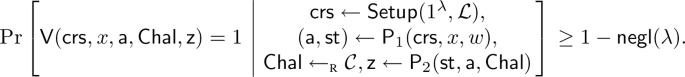
• Special zero-knowledge: There exists a PPT simulator ${\textsf{ZKSim}}$ such that for any $\textsf{crs}\in {\textsf{Setup}}(1^\lambda , \mathcal {L})$, any $(x,w) \in \mathcal {R}_{\textsf{zk}}$ and any challenge $\textsf{Chal}\in \mathcal {C}$, the following distributions are computationally indistinguishable:

  $$\begin{aligned} \{(\textsf{a}, \textsf{Chal},\textsf{z}) \mid (\textsf{a}, \textsf{z})&\leftarrow {\textsf{ZKSim}}(\textsf{crs}, x, \textsf{Chal})\} \approx _c\\ &\left\{ (\textsf{a},\textsf{Chal}, \textsf{z}) \, \left| \, (\textsf{a}, \textsf{st}) \leftarrow {\textsf{P}}_1(\textsf{crs}, x,w),\textsf{z}\leftarrow {\textsf{P}}_2(\textsf{st},\textsf{a}, \textsf{Chal}) \right\} . \right. \end{aligned}$$

• Special soundness: For any CRS $\textsf{crs}\in {\textsf{Setup}}(1^\lambda , \mathcal {L})$ , any $x \not \in \mathcal {L}_{\textsf{sound}}$, and any first prover’s message $\textsf{a}$, there exists at most one challenge $\textsf{Chal}= f(\textsf{crs},x,\textsf{a}) \in \mathcal {C}$ for which there exists a valid prover’s reply $\textsf{z}$, i.e., ${\textsf{V}}(\textsf{crs},x,\textsf{a},\textsf{Chal},\textsf{z})=1$. The function f is called the bad challenge function of $\varPi$.

Definition 2.9

(Trapdoor gap $\varSigma$-protocol). Let $\mathcal {L}= (\mathcal {L}_{\textsf{zk}}, \mathcal {L}_{\textsf{sound}})$ be a language associated with two NP relations $\mathcal {R}_{\textsf{zk}}, \mathcal {R}_{\textsf{sound}}$, s.t. $\mathcal {L}_{\textsf{zk}}\subseteq \mathcal {L}_{\textsf{sound}}$. A gap $\varSigma$-protocol $\varPi = ({\textsf{Setup}}, {\textsf{P}}, {\textsf{V}})$ for $\mathcal {L}$ with a bad challenge function f is a trapdoor gap $\varSigma$-protocol if there exist PPT algorithms $({\textsf{TrapSetup}}, {\textsf{BadChallenge}})$ with the following syntax:

• ${\textsf{TrapSetup}}(1^\lambda ,\mathcal {L}, \tau _\mathcal {L})$: Given public parameters $\textsf{par}$, language $\mathcal {L}$ and a membership trapdoor $\tau _\mathcal {L}$ for the language $\mathcal {L}_{\textsf{sound}}$ as input, it outputs a CRS $\textsf{crs}$ and a trapdoor $\tau _\varSigma \in \{0,1\} ^{\ell _\tau }$ for some $\ell _\tau (\lambda )$;

• ${\textsf{BadChallenge}}(\tau _\varSigma , \textsf{crs}, x, \textsf{a})$ : Given a trapdoor $\tau _\varSigma$, a CRS $\textsf{crs}$, a statement x and a first prover message $\textsf{a}$ as input, it outputs a challenge $\textsf{Chal}$;

and satisfying the following properties:

• CRS indistinguishability: For any trapdoor $\tau _\mathcal {L}$ for the language $\mathcal {L}_{\textsf{sound}}$, the following distributions are computationally indistinguishable

  $$ \{ \textsf{crs}\mid \textsf{crs}\leftarrow {\textsf{Setup}}(1^\lambda , \mathcal {L})\} \approx _c\{ \textsf{crs}\mid \textsf{crs}\leftarrow {\textsf{TrapSetup}}(1^\lambda , \mathcal {L}, \tau _\mathcal {L})\}. $$

• Correctness: There exists a language-specific trapdoor $\tau _\mathcal {L}$ s.t. for any instance $x \not \in \mathcal {L}_{\textsf{sound}}$, all pairs $(\textsf{crs}, \tau _\varSigma ) \in {\textsf{TrapSetup}}(1^\lambda , \mathcal {L}, \tau _\mathcal {L})$ and any first prover message $\textsf{a}$, we have ${\textsf{BadChallenge}}(\tau _\varSigma , \textsf{crs}, x, \textsf{a}) = f(\textsf{crs},x,\textsf{a})$.

Let us now recall the definition of a Non-Interactive Zero Knowledge (NIZK) proof. We closely follow the definition given by Libert et al. [36].

Definition 2.10

(NIZK). Let $\mathcal {L}= (\mathcal {L}_{\textsf{zk}}, \mathcal {L}_{\textsf{sound}})$ be a language associated with two NP relations $\mathcal {R}_{\textsf{zk}}$, $\mathcal {R}_{\textsf{sound}}$, such that $\mathcal {L}_{\textsf{zk}}\subseteq \mathcal {L}_{\textsf{sound}}$ and statements are of bit-length N. A non-interactive zero-knowledge (NIZK) argument system $\varPi$ for a language $\mathcal {L}$ consists of three PPT algorithms $({\textsf{Setup}}, {\textsf{P}}, {\textsf{V}})$ with the following syntax:

• ${\textsf{Setup}}(1^\lambda , \mathcal {L}, \tau _\mathcal {L}):$ Given an unary encoded security parameter $\lambda$, a language $\mathcal {L}$ and a membership testing trapdoor $\tau _\mathcal {L}$ for $\mathcal {L}$ as input, it outputs a CRS $\textsf{crs}$.

• ${\textsf{P}}(\textsf{crs}, x, w)$: Given a CRS $\textsf{crs}$, a statement $x \in \{0,1\} ^N$, and a witness w as input, the proving algorithm outputs a proof $\pi$.

• ${\textsf{V}}(\textsf{crs}, x, \pi )$ : Given a CRS $\textsf{crs}$, a statement $x \in \{0,1\} ^N$, and a proof $\pi$ as input, the verification algorithm outputs a decision bit.

Moreover, $\varPi$ should satisfy the following properties.

Completeness: For any $(x,w)\in \mathcal {R}_{\textsf{zk}}$, any $\textsf{lbl}\in \{0,1\} ^*$ and any membership testing trapdoor $\tau _\mathcal {L}$ for $\mathcal {L}$, we have

$$\begin{aligned} \Pr [{\textsf{V}}(\textsf{crs},x,\pi )=1 \mid \textsf{crs}\leftarrow {\textsf{Setup}}(1^\lambda , \mathcal {L}, \tau _\mathcal {L}), \pi \leftarrow {\textsf{P}}(\textsf{crs}, x, w)] \ge 1-\textsf{negl}(\lambda ). \end{aligned}$$

Soundness: For any $x \in \{0,1\} ^N \setminus \mathcal {L}_{\textsf{sound}}$, any membership testing trapdoor $\tau _\mathcal {L}$ for $\mathcal {L}$ and any PPT prover ${\textsf{P}}^*$, we have

$$ \Pr [ {\textsf{V}}(\textsf{crs}, x, \pi )=1 \mid \textsf{crs}\leftarrow {\textsf{Setup}}(1^\lambda , \mathcal {L}, \tau _\mathcal {L}), \pi \leftarrow {\textsf{P}}^*(\textsf{crs}, x)] \le \textsf{negl}(\lambda ). $$

Zero-Knowledge: There is a PPT simulator $({\textsf{Sim}}_0, {\textsf{Sim}}_1)$ such that for any PPT adversary $\mathcal {A}$, we have that for all trapdoors $\tau _\mathcal {L}$:

$$\begin{aligned} {} & {} \vert \Pr [1\leftarrow \mathcal {A}^{\mathcal {O}_{{\textsf{P}}}(\textsf{crs}, \cdot , \cdot )}(\textsf{crs}) \mid \textsf{crs}\leftarrow {\textsf{Setup}}(1^\lambda , \mathcal {L}, \tau _\mathcal {L})] \\ {} & {} \qquad \qquad - \Pr [1\leftarrow \mathcal {A}^{\mathcal {O}_{{\textsf{Sim}}}(\textsf{crs}, \tau _\textsf{zk}, \cdot , \cdot )}(\textsf{crs}) \mid (\textsf{crs}, \tau _\textsf{zk})\leftarrow {\textsf{Sim}}_0(1^\lambda , \mathcal {L})] \vert \le \textsf{negl}(\lambda ), \end{aligned}$$

where $\mathcal {O}_{{\textsf{P}}}(\textsf{crs}, x,w)$ outputs $\bot$ if $(x,w) \not \in \mathcal {R}_{\textsf{zk}}$ and $\pi \leftarrow {\textsf{P}}(\textsf{crs}, x,w)$ otherwise, and $\mathcal {O}_{{\textsf{Sim}}}(\textsf{crs}, \tau _\textsf{zk}, x, w)$ outputs $\bot$ if $(x,w) \not \in \mathcal {R}_{\textsf{zk}}$ and ${\textsf{Sim}}_1(\textsf{crs}, \tau _\textsf{zk},x)$ otherwise.

Finally we recall the standard definition for digital signature and a public key encryption scheme.

Definition 2.11

(Digital Signature). A digital signature scheme $\varSigma$ for a message space $\mathcal {M}$ and signature space $\mathbb {S}$ consist of three PPT algorithms $({\textsf{KeyGen}},{\textsf{Sign}},{\textsf{Ver}})$ with the following syntax

• ${\textsf{KeyGen}}(1^\lambda )$: Given an unary encoded security parameter $\lambda$ as input, it outputs a verfication key $\textsf{vk}$ and a signing key $\textsf{sk}$.

• ${\textsf{Sign}}(\textsf{sk},\textsf{msg})$: Given a signing key $\textsf{sk}$ and a message $\textsf{msg}\in \mathcal {M}$ as input, it outputs a signature $\textsf{sig}\in \mathbb {S}$.

• ${\textsf{Ver}}(\textsf{vk},\textsf{msg},\textsf{sig})$: Given a verification key $\textsf{vk}$, a message $\textsf{msg}\in \mathcal {M}$ and a signature $\textsf{sig}\in \mathbb {S}$ as input, it outputs 1 (indicating a valid signature) or 0 (indicating an invalid signature).

A digital signature scheme $\varSigma =({\textsf{KeyGen}},{\textsf{Sign}},{\textsf{Ver}})$ is correct, if for every message $\textsf{msg}\in \mathcal {M}$, we have

$$\begin{aligned} {} & {} \vert \Pr [{\textsf{Ver}}(\textsf{vk},\textsf{msg},\textsf{sig})= 1 \mid (\textsf{vk},\textsf{sk}) \leftarrow {\textsf{KeyGen}}(1^\lambda ), \textsf{sig}\leftarrow {\textsf{Sign}}(\textsf{sk},\textsf{msg})] \vert \\ {} & {} \qquad \qquad \qquad \qquad \qquad \qquad \qquad \qquad \qquad \qquad \qquad \,\qquad \qquad \,\,\,\, \ge 1- \textsf{negl}(\lambda ). \end{aligned}$$

Definition 2.12

(Public-Key Encryption). A public key encryption scheme $\varPi$ for a message space $\mathcal {M}$ consist of three PPT algorithms $({\textsf{KeyGen}},{\textsf{Enc}},{\textsf{Dec}})$ with the following syntax

• ${\textsf{KeyGen}}(1^\lambda )$ : Given an unary encoded security parameter $\lambda$ as input, it outputs a public key $\textsf{pk}$ and a secret key $\textsf{sk}$.

• ${\textsf{Enc}}(\textsf{pk},\textsf{msg})$ : Given a public key $\textsf{pk}$ and a message $\textsf{msg}\in \mathcal {M}$ as input, it outputs a ciphertext $\textsf{ct}$.

• ${\textsf{Dec}}(\textsf{sk},\textsf{ct})$ : Given a secret key $\textsf{sk}$ and a ciphertext $\textsf{ct}$ as input, it outputs a message $\textsf{msg}\in \mathcal {M}$ or $\bot$ (indicating a failure).

A PKE scheme $\varPi =({\textsf{KeyGen}},{\textsf{Enc}},{\textsf{Dec}})$ is correct, if for every $\textsf{msg}\in \mathcal {M}$, we have

$$\begin{aligned} \vert \Pr [{\textsf{Dec}}(\textsf{sk},\textsf{ct})= \textsf{msg}\mid (\textsf{pk},\textsf{sk}) \leftarrow {\textsf{KeyGen}}(1^\lambda ), \textsf{ct}\leftarrow {\textsf{Enc}}(\textsf{pk},\textsf{msg})] \vert \ge 1- \textsf{negl}(\lambda ). \end{aligned}$$

3 Structure-Preserving Sets

The first building block in our framework is the notion of a structure-preserving set, which is a crucial tool in capturing the defining characteristics of a specific family of lattice-based signatures, encryption schemes and NIZKs which are compatible with each other. The properties that lead to such structure-preserving cryptographic primitives are described in later sections.

Let q be a large prime. A structure-preserving set S is a special subset of $\mathbb {Z}_q^d$ that can be rerandomized to obtain a rerandomized set $S'=S+D$ (where D is a set which contains the rerandomizing terms). Given a vector $\mathbf {{s}}\in S$, we can rerandomize $\mathbf {{s}}$ to obtain $\mathbf {{s}}'\in S+D$. The structure-preserving property of S ensures that given $\mathbf {{s'}}$, one is able to check whether the original vector $\mathbf {{s}}\in \mathbb {Z}_q^d$ belonged to S or whether it lied outside of S. In particular, vector $\mathbf {{s}}'$ allows to check membership of the original $\mathbf {{s}}$, but it hides its original value.

Definition 3.1

(Uniformly Structure-Preserving Set). We say that a set $S\subseteq \mathbb {Z}_{q}^d$ is uniformly structure-preserving if (i) there exists a subset $D \subseteq \mathbb {Z}_q^d$ such that for all messages $\mathbf {{s}},\mathbf {{s}}'\in S$

(ii) for $\overline{S} :=\mathbb {Z}_{q}^d\setminus S$ it holds that $(S+ D) \cap (\overline{S} + D) = \emptyset$, and the membership problem for D and $S+ D$ are easy and we can efficiently sample uniformly at random from D. We call the maximal statistical distance between the first two boxed distributions the structure-preserving error.

To provide some intuition about the introduced notion, let us demonstrate the definition of a concrete example that we use later in the paper. Namely, we show that cosets of subgroups are uniformly structure-preserving.

Example 3.2

(Cosets of subgroups). Every coset $S$ of an additive subgroup $G\le \mathbb {Z}_{q}^d$ is uniformly structure-preserving.

Proof

By definition of a coset, all the sets $S_{\mathbf {{s}}} = \{\mathbf {{s}}+ \mathbf {{d}}\mid \mathbf {{d}}\in G\}$ (for $\mathbf {{s}}\in S$) are the same set $S$ again. Thus by picking $D:=G$, we get that for all $\mathbf {{s}},\mathbf {{s}}'\in S$, $\mathbf {{s}}+ \mathbf {{d}}$ and $\mathbf {{s}}' + \mathbf {{d}}$ for $\mathbf {{d}}\leftarrow _{\textsc {r}}D$ are identically distributed. Hence the first part of the definition is satisfied and the structure-preserving error is 0.

For $\mathbf {{x}}\in \mathbb {Z}_{q}^d\setminus S$, we know that $\mathbf {{x}}\in S'$ for $S'\ne S$ being another coset of G. Thus for every $\mathbf {{d}}\in G$, we have $\mathbf {{x}}+ \mathbf {{d}}\in S'$. Since different cosets are disjoint, the second part of the definition is satisfied as well.   $\square$

Remark 3.3

The above example, in particular, implies that

• 1. all additive subgroups of $\mathbb {Z}_q^d$ are uniformly structure-preserving; and

• 2. all singleton sets are uniformly structure-preserving, because they are cosets of the trivial subgroup $\{\mathbf {{0}}\}$.

In order to define lattice-based structure-preserving signatures and encryptions, we will need a more generic definition of a structure-preserving set. Namely, we do not want to restrict ourselves to $\mathbf {{d}}$ being sampled uniformly at random, but from any distribution on $\mathbb {Z}_q^d$. Looking ahead, since we work with lattice-based primitives, we are particularly interested in Gaussian distributions. Along with the change of distribution for $\mathbf {{d}}$, we generalize the definition by loosening some of its condition. At a high level, in both the first and the second part of the definition, we allow for small errors with some probability.

Definition 3.4

(Structure-Preserving Set). We say that a set $S\subseteq \mathbb {Z}_{q}^d$ is structure-preserving with noise growth $\delta$ if there exists an efficiently sampleable probability distribution $\mathcal {D}$ on $\mathbb {Z}_{q}^{d}$, a constant $\alpha \in (0,1]$, that we will call the no-abort constant, and a function $\textsf{success}:S\times S\times \mathop {\textrm{supp}}\limits (\mathcal {D})\rightarrow (0,1]$, that we will call the no-abort function, such that (i) for all messages $\mathbf {{s}},\mathbf {{s}}'\in S$

and (ii) there exists a set $D'\subseteq \mathbb {Z}_{q}^{d}$, that we will call the smudging set, such that $\Pr _{\mathbf {{d}}\leftarrow \mathcal {D}}[\mathbf {{d}}\in D'] \ge 1 - \textsf{negl}(\lambda )$ for a negligible function $\textsf{negl}$, and for $\overline{S}_{\delta }:=\mathbb {Z}_{q}^d\setminus B_{\delta }(S)$, it holds that $\left( S+ D'\right) \cap \left( \overline{S}_{\delta } + D'\right) = \emptyset$. Moreover, the membership problem for $D'$ and $(S+ D')$ are easy.¹¹ We call $\textsf{negl}$ the soundness error.

It is easy to see that uniformly structure-preserving sets are special cases of structure-preserving sets.

Lemma 3.5

Let S be an uniformly structure-preserving set. Then S is a structure-preserving set with noise growth 0 and soundness error 0.

Proof

By setting $\mathcal {D}$ to be the uniform distribution on D, $\textsf{success}$ to be the constant function 1, $\alpha :=1$ and $D'= D$, we directly obtain that S is a structure-preserving with noise growth 0 and soundness error 0.    $\square$

Let us provide an example of a structure-preserving set which is not uniformly structure-preserving.

Example 3.6

(Close vectors). Every set $S\subseteq \mathbb {Z}_{q}^{d}$ where $S-S$ is T-bounded (i.e., $S-S\subseteq B_{T}(\{\mathbf {{0}}\})$) is structure-preserving with noise growth $4Td+ 1$, when $d$ grows polynomially with the security parameter.

Proof

Pick $\mathcal {D}:=\mathcal {D}_{\mathbb {Z}^{d},\sigma }$ with $\sigma :=T\sqrt{d}$. For all $\mathbf {{s}},\mathbf {{s}}'\in S$, by Lemma 2.7, the distribution that outputs $\mathbf {{s}}- \mathbf {{s}}' + \mathbf {{d}}$ for $\mathbf {{d}}\leftarrow \mathcal {D}_{\mathbb {Z}^{d},\sigma }$ with probability $\textsf{success}(\mathbf {{s}},\mathbf {{s}}',\mathbf {{d}}):=\min \left( \frac{\rho _{\mathbb {Z}^d,\sigma }(\mathbf {{s}}- \mathbf {{s}}' + \mathbf {{d}})}{M\rho _{\mathbb {Z}^d,\sigma }(\mathbf {{d}})},1\right)$ is statistically close to outputting $\mathbf {{d}}\leftarrow \mathcal {D}_{\mathbb {Z}^{d},\sigma }$ with probability $\alpha :=1/M$ for a constant M. By adding $\mathbf {{s}}'$ to the output of these two distributions, we get that the first condition for a structure-preserving set is satisfied.

Pick $D':=B_{2Td}(\{\mathbf {{0}}\})$ as smudging set. By the tail bound for Gaussian distributions (Lemma 2.1) we have $\Pr _{\mathbf {{d}}\leftarrow \mathcal {D}_{\mathbb {Z}^{d},\sigma }}[\Vert \mathbf {{\mathbf {{d}}}}\Vert >2Td] < 2^{d}e^{\frac{-3d}{2}} = \left( 2e^{-3/2}\right) ^{d} < \frac{1}{2^{d}},$ which shows that this choice is valid. For $\mathbf {{x}}\in \overline{S}_{\delta } := \mathbb {Z}_{q}^d\setminus B_{4Td+1}(S)$ and $\mathbf {{d}}\in D'$ we have $\mathbf {{x}}+ \mathbf {{d}}\in \mathbb {Z}_{q}^d\setminus B_{2Td}(S)$. On the other hand, for $\mathbf {{s}}\in S$ we have $\mathbf {{s}}+\mathbf {{d}}\in B_{2Td}(S).$ This implies that $( S+ D')\cap ( \overline{S}_{\delta } + D') = \emptyset$ which is the second condition for a structure-preserving set.    $\square$

Remark 3.7

This example, in particular, implies that sets of small vectors are structure-preserving. Namely, let $S\subseteq \mathbb {Z}_{q}^{d}$ be a T-bounded set. Then by triangular inequality, $S - S$ is 2T-bounded and hence S structure-preserving with noise growth $8Td+1$.

Next, we show that structure-preserving sets are closed under the cartesian product.

Example 3.8

When $S_{1}\subseteq \mathbb {Z}_{q}^{d_{1}}$ is a structure-preserving set with noise growth $\delta _{1}$ and $S_{2}\subseteq \mathbb {Z}_{q}^{d_{2}}$ is a structure-preserving set with noise growth $\delta _{2}$, then $S_{1} \times S_{2}\subseteq \mathbb {Z}_{q}^{d_{1}+d_{2}}$ is structure-preserving with noise $\max \{\delta _{1},\delta _{2}\}$.

Proof

Let $\mathcal {D}_{1},\textsf{success}_{1},\alpha _{1}$ be the distribution, abort function and abort constant that make $S_{1}$ a structure-preserving set with noise $\delta _{1}$ and $\mathcal {D}_{2},\textsf{success}_{2},\alpha _{2}$ be the distribution, abort function and abort constant that make $S_{2}$ a structure-preserving set with noise $\delta _{2}$. Then the distribution $\mathcal {D}_{1} \times \mathcal {D}_{2}$ with the success function

$$\begin{aligned} \textsf{success}((\mathbf {{m}}_{1},\mathbf {{m}}_{2}),(\mathbf {{m}}_{1}',\mathbf {{m}}_{2}'),\mathbf {{d}}):=\textsf{success}_{1}(\mathbf {{m}}_{1},\mathbf {{m}}_{1}',\mathbf {{d}})\cdot \textsf{success}_{2}(\mathbf {{m}}_{2},\mathbf {{m}}_{2}',\mathbf {{d}}) \end{aligned}$$

and success probability constant $\alpha :=\alpha _{1}\alpha _{2}$ makes the set $S_{1} \times S_{2}$ structure-preserving with noise $\max \{\delta _{1},\delta _{2}\}$.    $\square$

We complete this section with an alternative formulation of the structure-preserving set property that is easier to use in some of the proofs.

Lemma 3.9

For a structure-preserving set $S$ with noise growth $\delta$ and smudging set $D'$ we have $S+ D'- D'\subseteq B_{\delta }(S).$

Proof

We prove this Lemma by contradiction. Suppose there exist $\mathbf {{s}}\in S$ and $\mathbf {{d}},\mathbf {{d}}' \in \mathcal {D}$ such that $\mathbf {{x}}:= \mathbf {{s}}+ \mathbf {{d}}- \mathbf {{d}}' \notin B_{\delta }(S)$, i.e. $\mathbf {{x}}\in \overline{S}_\delta :=\mathbb {Z}_{q}^d\setminus B_{\delta }(S)$. But then

$$ S+ D'\ni \mathbf {{s}}+ \mathbf {{d}}= \mathbf {{x}}+ \mathbf {{d}}' \in \overline{S}_\delta + D', $$

which is in contradiction to part (ii) of Definition 3.4.    $\square$

4 Lattice-Based Structure-Preserving Signatures

A lattice-based structure-preserving signature ($\textsf{SPS}$) scheme $\varSigma$ expresses its verification algorithm in the framework of structure-preserving sets. Namely, a signature $\sigma$ can be split into two separate parts $\sigma =(\textsf{core},\textsf{tag})$. In order to verify that $\sigma$ is valid, the $\varSigma$ verification algorithm checks whether $f(\textsf{core})$ belongs to a structure-preserving set S. The function f is publicly computable from $\textsf{tag}$, along with public verification key $\textsf{vk}$ and the message m.

The requirement to use $\textsf{tag}$ arises from specific properties of known lattice-based $\textsf{SPS}$ schemes. The $\textsf{tag}$ is publicly samplable and, for example, it could be a random string. At a technical level, the $\textsf{tag}$ is usually required in all known lattice-based signatures that satisfy strong-unforgeability, and can remain unused in some schemes that are only existentially-unforgeable.

Definition 4.1

(Lattice SPS). A lattice-based $\mathcal {F}$-structure-preserving signature $\varSigma$ for a family $\mathcal {F}$ of functions ${f}:\mathbb {S}\rightarrow \mathbb {Z}_{q}^{d'}$ is a digital signature with signature space $\mathbb {S}\times \mathbb {T}$ where for every verification key $\textsf{vk}$, every message $\textsf{msg}$ and every signature $(\textsf{core},\textsf{tag})\in \mathbb {S}\times \mathbb {T}$

$$ {\textsf{Ver}}(\textsf{vk},\textsf{msg},(\textsf{core},\textsf{tag})) = 1 \Longleftrightarrow f(\textsf{core})\in S$$

where $f\in \mathcal {F}$ and $S\subseteq \mathbb {Z}_{q}^{d'}$ are derived from $\textsf{vk}$, $\textsf{msg}$ and $\textsf{tag}$. Furthermore, $S$ is a structure-preserving set. Finally, we require that tags are publicly samplable. That is, there exists an algorithm ${\textsf{TagGen}}$ that, given the verification key $\textsf{vk}$ and a message $m$ generates a tag $\textsf{tag}$ that has the same distribution as the tag part of the signatures generate with the signing algorithm.

Fig. 1.

Security experiment for and security of lattice-based structure-preserving signatures.

Remark 4.2

Since we do not require the membership problem for the sets $S$ to be easy, this definition does not give immediately rise to an alternative verification procedure.

We are particularly interested in the cases where $\mathcal {F}$ is the set of linear functions or the set of functions that can be computed by bounded-depth Boolean circuits after encoding the signature as a binary string.

For structure-preserving signatures we require a slightly stronger security notion (defined below) than standard (strong) existential unforgeability under chosen message attacks ($\mathsf {(s)EUF\hbox {-}{}CMA}$). Compared to $\mathsf {(s)EUF\hbox {-}{}CMA}$, we relax the verification of the forged signature as follows: Instead of requiring that the forged signature $\textsf{sig}=(\textsf{core},\textsf{tag})$ satisfies $f(\textsf{core})\in S$, we only require $f(\textsf{core})\in B_{\delta _{S}}(S)$.

Definition 4.3

($\mathsf {SPS\hbox {-}{}(s)EUF\hbox {-}{}CMA}$). We call a structure-preserving signature scheme $({\textsf{KeyGen}},{\textsf{Sign}},{\textsf{Ver}})$ $\mathsf {SPS\hbox {-}{}EUF\hbox {-}{}CMA}$ or $\mathsf {SPS\hbox {-}{}sEUF\hbox {-}{}CMA}$-secure, if every PPT adversary can win the respective game in Fig. 1 with at most negligible probability.

4.1 SPS Instantiation

Examples of structure-preserving signatures are Boyen’s signature scheme [14], Rückert’s signature scheme [46] and a new scheme, that combines the advantages of these two schemes. Namely, it achieves strong unforgeablity and has a simpler verification (because it does not need the non-zero signature check). Furthermore, it is more efficient (due to shorter signatures) than Rückert’s scheme. We only show that the new scheme satisfies Definition 4.1 here and present the remaining details in the full version.

As a prerequisite, we state some facts that are needed in the signature scheme description, and define and construct chameleon hash functions.

Fact 1

([14, Fact 5]). There is a PPT algorithm ${\textsf{TrapGen}}$ that, on input the security parameter $\lambda$, an odd prime $q= \textsf{poly}(\lambda )$, and two integers $n=\varTheta (\lambda )$ and $m\ge 6n\log q$, outputs a matrix $\mathbf {{A}} \in \mathbb {Z}_q^{n\times m}$ statistically close to uniform, and a basis $\mathbf {{T}}_{\mathbf {{A}}}$ for $\varLambda ^\bot (\mathbf {{A}})$ such that $\Vert \bar{\mathbf {{T}}}_{\mathbf {{A}}}\Vert \le \tilde{\varTheta }(\sqrt{m}) \le L$ with overwhelming probability. We assume $L= \tilde{\varOmega }(\sqrt{m})$.

Fact 2

([14, Lemma 22]). For a security parameter $\lambda$, let $q= \textsf{poly}(\lambda )$ be an odd prime, $n=\varTheta (\lambda )$, $m\ge 6n\log q$, $L=\tilde{\varOmega }(\sqrt{m})$ and $\sigma \ge L\omega (\sqrt{\log m})$. Then there exist a PPT algorithm ${\textsf{SamplePre}}$ that on input a Gaussian parameter $\sigma$, a modulus $q$, a matrix $\mathbf {{F}}:=[\mathbf {{A}}|\mathbf {{B}}] \leftarrow _{\textsc {r}}\mathbb {Z}_q^{n\times 2m}$, and a basis $\mathbf {{T}}_{\mathbf {{A}}}\subset \varLambda ^\bot (\mathbf {{A}})$ of norm $\Vert \bar{\mathbf {{T}}}_{\mathbf {{A}}}\Vert \le L$, and a vector $\mathbf {{u}}$, outputs $\mathbf {{d}} \in \varLambda ^\bot (\mathbf {{F}})$ from the distribution $\mathcal {D}_{\mathbb {Z}^{m},\sigma }$ conditioned on $\mathbf {{F}}\mathbf {{d}}= \mathbf {{u}}$.

Fact 3

([4, Section 4.2]). Given matrices $\mathbf {{A}},\mathbf {{B}}\in \mathbb {Z}_q^{n \times m}$, $\mathbf {{B}}$ needs to have rank n, a short basis $\mathbf {{T}}_\mathbf {{B}}$ for $\mathbf {{B}}$ and a short matrix $\mathbf {{R}}\in \mathbb {Z}_q^{m \times m}$, one can compute efficiently a short basis $\mathbf {{T}}_\mathbf {{F}}$ for $\mathbf {{F}}:= (\mathbf {{A}}\vert \mathbf {{A}}\mathbf {{R}}+ \mathbf {{B}})$ with $\Vert \widetilde{\mathbf {{T}}_\mathbf {{F}}} \Vert \le \Vert \widetilde{\mathbf {{T}}_\mathbf {{B}}}\Vert (\Vert \mathbf {{R}}\Vert + 1)$.

Definition 4.4

(Chameleon hash function). A chameleon hash function with message space $\mathcal {M}$ and hash space $\mathcal {N}$ consists of an efficiently sampable distribution $\mathcal {R}$ on some randomness space $R$ and two PPT algorithms $({\textsf{GenCH}},{\textsf{TrapColl}})$ with the following syntax

• ${\textsf{GenCH}}(1^\lambda )$ : Given an unary encoded security parameter $\lambda$ as input, it outputs an efficiently computable chameleon hash function $\textsf{ch}:\mathcal {M}\times R\rightarrow \mathcal {N}$ and a trapdoor $\tau$.

• ${\textsf{TrapColl}}(\tau ,m\in \mathcal {M},r\in R,m^*\in \mathcal {M})$ : Given the trapdoor $\tau$ for a chameleon hash function $\textsf{ch}$, two messages $m,m^*$ and one randomness r this algorithm outputs $r^*$ such that $\textsf{ch}(m,r) = \textsf{ch}(m^*,r^*)$ and $r^*$ is distributed according to $\mathcal {R}$.

The security property we require for chameleon hash functions is collision resistance. That is, for every PPT adversary $\mathcal {A}$, the following probability is negligible

$$\begin{aligned} {} & {} \Pr [(\textsf{ch},\tau )\leftarrow _{\textsc {r}}{\textsf{GenCH}},(m,r,m^*,r^*)\leftarrow _{\textsc {r}}\mathcal {A}(1^\lambda ,\textsf{ch}):\textsf{ch}(m,r)=\textsf{ch}(m^*,r^*) \\ {} & {} \qquad \qquad \qquad \qquad \qquad \qquad \qquad \qquad \qquad \qquad \qquad \,\,\,\,\,\,\,\,\,\,\,\,\, \, \wedge (m,r) \ne (m^*,r^*)]. \end{aligned}$$

An example of a chameleon hash function based on the SIS assumption is by [18]. It has message space $\mathcal {M}:=\{0,1\}^k$ and randomness space $R:=\{\mathbf {{r}}\in \mathbb {Z}^{m} \mid \Vert \mathbf {{r}}\Vert < s \sqrt{m}\}$ with a tail-truncated discrete Gaussian distribution $\mathcal {D}_{R,s}$ where $s = L\cdot \omega (\sqrt{\log m})$ and n, m, and $L$ are as in Fact 1. It works as follows:

• ${\textsf{GenCH}}(1^\lambda )$ samples $\mathbf {{A}}_{0}\leftarrow _{\textsc {r}}\mathbb {Z}_{q}^{n\times k}$ and $\mathbf {{A}}_{1}\in \mathbb {Z}_{q}^{n\times m}$ with short basis $\mathbf {{S}}$ using ${\textsf{TrapGen}}$. Output $\mathbf {{A}}:=(\mathbf {{A}}_{0}|\mathbf {{A}}_{1})$ to describe the chameleon hash function

  $$\begin{aligned} \textsf{ch}_\mathbf {{A}}:\{0,1\}^k \times R&\rightarrow \mathbb {Z}_{q}^{n}\\ (\mathbf {{m}},\mathbf {{r}}) & \mapsto \mathbf {{A}}\cdot \begin{pmatrix} \mathbf {{m}}\\ \mathbf {{r}}\end{pmatrix} \end{aligned}$$

• ${\textsf{TrapColl}}(\tau ,\mathbf {{m}}\in \mathcal {M},\mathbf {{r}}\in R,\mathbf {{m}}^*\in \mathcal {M})$ samples and outputs a vector $\mathbf {{r}}^*$ according to (a distribution statistically close to) $\mathcal {D}_{R,s}$ condition on $\textsf{ch}_\mathbf {{A}}(\mathbf {{m}}^*,\mathbf {{r}}^*) = \textsf{ch}_\mathbf {{A}}(\mathbf {{m}},\mathbf {{r}})$ using Fact 2.

Lemma 4.5

([18, Lemma 4.1]). The above chameleon hash function is collision-resistant under the $\textsf{SIS}_{m,n,q,\beta }$ problem where $\beta :=\sqrt{k+4s^{2}m}$.

The ISIS-based signature scheme requires a chameleon hash function $({\textsf{GenCH}},{\textsf{TrapColl}})$ with message space $\mathcal {M}$, randomness space $R$ and hash space $\mathcal {N}= \{0,1\} ^\ell$ and is described as follows:

• ${\textsf{KeyGen}}(1^\lambda )$ : Given unary encoded security parameter $\lambda$ as input, proceed as follows:

  • 1. Execute the ${\textsf{TrapGen}}$ algorithm to obtain a matrix $\mathbf {{A}}\in \mathbb {Z}_q^{n\times m}$ and a basis $\mathbf {{T}}_{\mathbf {{A}}}\in \varLambda ^\top (\mathbf {{A}})$ such that $\Vert \bar{\mathbf {{T}}}_{\mathbf {{A}}}\Vert \le L$.

  • 2. Sample $\mathbf {{y}}\leftarrow _{\textsc {r}}\mathbb {Z}_q^n$, $(\mathbf {{C}}_0, \dots , \mathbf {{C}}_\ell ) \leftarrow _{\textsc {r}}\mathbb {Z}_q^{n\times m} \times \dots , \mathbb {Z}_q^{n\times m}$.

  • 3. Sample $(\textsf{ch},\tau )\leftarrow _{\textsc {r}}{\textsf{GenCH}}(1^\lambda )$.

  • 4. Output $\textsf{vk}:=(\mathbf {{A}}, \mathbf {{C}}_0, \dots , \mathbf {{C}}_\ell , \mathbf {{y}}, \textsf{ch})$ and $\textsf{sk}:=\mathbf {{T}}_{\mathbf {{A}}}$.

• ${\textsf{Sign}}(\textsf{sk},\textsf{msg})$ : Given a signing key $\textsf{sk}= \mathbf {{T}}_{\mathbf {{A}}}$ and a message $\textsf{msg}\in \mathcal {M}$ as input proceed as follows:

  • 1. Sample $r \leftarrow \mathcal {R}$ and set $\textsf{msg}':= \textsf{ch}(\textsf{msg}, r)$.

  • 2. Compute $\mathbf {{C}}_\textsf{msg}:=\mathbf {{C}}_0 + \sum _{i = 1}^{\ell } \textsf{msg}'_i \mathbf {{C}}_i$ and set $\mathbf {{F}}_{\textsf{msg}}:=[\mathbf {{A}}\mid \mathbf {{C}}_\textsf{msg}] \in \mathbb {Z}_q^{n\times 2m}$.

  • 3. Execute the algorithm ${\textsf{SamplePre}}$ on $\mathbf {{F}}_{\textsf{msg}}$, $\mathbf {{T}}_{\mathbf {{A}}}$ and $\sigma \ge 2L \omega (\sqrt{\log m})$ to obtain a short non-zero random point $\mathbf {{d}}$ with $\mathbf {{F}}_{\textsf{msg}}\mathbf {{d}}= \mathbf {{y}}$.

  • 4. Output the signature $\textsf{sig}:=(\textsf{core}=\mathbf {{d}},\textsf{tag}=r)$.

• ${\textsf{Ver}}(\textsf{vk},\textsf{msg},\textsf{sig})$ : Given a verification key $\textsf{vk}=(\mathbf {{A}}, \mathbf {{C}}_0, \dots , \mathbf {{C}}_\ell , \mathbf {{y}}, \textsf{ch})$, a message $\textsf{msg}\in \mathcal {M}$ and signature $\textsf{sig}=(\mathbf {{d}}\in \mathbb {Z}_q^{2m},r)$ as input, set $\textsf{msg}' := \textsf{ch}(\textsf{msg}, r)$ and output 1 if (1) $\Vert \mathbf {{d}}\Vert \le \sqrt{2m} \cdot \sigma$ and (2) $[\mathbf {{A}}\mid \mathbf {{C}}_0 + \sum _{i = 1}^{\ell } \textsf{msg}'_i \mathbf {{C}}_i] \mathbf {{d}}= \mathbf {{y}}\mod q$. Otherwise, output 0.

Lemma 4.6

The ISIS-based signature scheme from above is a SPS scheme.

Proof

A signature $\textsf{sig}$ is of the form $(\textsf{core},\textsf{tag}) = (\mathbf {{d}},r)$. Clearly, these tags are publicly samplable.

According to definition Definition 4.1, what remains to show is that the signature verification can be expressed as $f(\textsf{core}) \in S$ for some function $f: \mathbb {Z}_q^{2m} \rightarrow \mathbb {Z}_{q}^{d'}$ and some set $S \subseteq \mathbb {Z}_q^{d'}$ which is structure-preserving. Both the function $f$ and the set S might depend on the message being signed, the verification key and the public parameters of the scheme. We show that the signature verification can be expressed as two checks of the type $f_i(\textsf{core}) \in S_i$ ($i \in \{1,2\}$). These check can then be combined to a single check by setting $f(\textsf{core}) := (f_1(\textsf{core}),f_2(\textsf{core}))$ and $S := S_{1} \times S_{2}$. The set S is structure-preserving when $S_{1}$ and $S_{2}$ are structure-preserving by Example 3.8.

The first check is $\Vert \textsf{core}\Vert \le \sqrt{2m} \cdot \sigma$, i.e., that $\textsf{core}$ is a small vector. For this, we can set $n_1':=2m$ and

$$ f_1(\textsf{core}) :=\textsf{core}, \quad \text {and} \quad S_1:=\{\mathbf {{x}}\in \mathbb {Z}_q^{2m} \mid \Vert \mathbf {{x}}\Vert \le \sqrt{2m} \cdot \sigma \} = B_{\sqrt{2m} \cdot \sigma }(\{0\}). $$

By triangular inequality, we have that $S_1-S_1 \subseteq B_{2\sqrt{2m} \cdot \sigma }(\{0\})$. By Remark 3.7, we can conclude that $S_1$ is structure-preserving with noise growth $16 m\sigma +1$.

For the second check, we can set $n_2' :=n$ and

$$\begin{aligned} f_2(\textsf{core})&:=\left[ \mathbf {{A}}\left| \mathbf {{C}}_0 + \sum _{i = 1}^{\ell } \textsf{msg}_i \mathbf {{C}}_i\right] \textsf{core}\right. \quad \text {and} \quad S_2 :=\{\mathbf {{y}}\} \subset \mathbb {Z}_q^{n}. \end{aligned}$$

Note that the function $f_2$ is defined by the message and the verification key. Moreover, $S_2$ is a singleton set and hence by Remark 3.3 and Lemma 3.5, we know that it is structure-preserving with noise growth 0.    $\square$

We prove $\mathsf {SPS\hbox {-}{}sEUF\hbox {-}{}CMA}$-security of our scheme in the full version.

5 Lattice-Based Structure-Preserving Encryption

Our notion of a structure-preserving encryption ($\textsf{SPE}$) captures the common properties of known lattice-bases encryption schemes which are compatible with efficient lattice-based sigma protocols and NIZKs that prove statements about ciphertexts. In particular, the randomness space needs to be a structure-preserving set (Definition 3.4) and ciphertexts are of the form $\textsf{ct}=\mathbf {{B}}_{\alpha }\mathbf {{r}}+g_\alpha (\textsf{msg})$, where $\mathbf {{B}}_{\alpha }$ is a public matrix depending on the message dimension $\alpha$, and $g_\alpha$ is an invertible encoding function.

In addition, $\textsf{SPE}$ needs to satisfy a series of technical properties on the noise, which provides bounds on the noise levels. This is a crucial property that allows for compatibility with the sigma protocols in later sections.

Definition 5.1

(Lattice SPE). A PKE scheme $({\textsf{KeyGen}},{\textsf{Enc}},{\textsf{Dec}})$ is a lattice-based structure-preserving encryption scheme if it satisfies the following properties:

• It has message space $\mathcal {M}^*$ for some base set $\mathcal {M}$. That is, we can encrypt arbitrary dimensional vectors of some base set $\mathcal {M}$. The ciphertexts will reveal the dimensions of the vectors.

• Public key: The public key implicitly defines matrices $(\mathbf {{B}}_{\alpha }\in \mathbb {Z}_{q}^{d(\alpha )\times r(\alpha )})_{\alpha \in \mathbb {N}_+}$ and efficiently sampleable distribution $(\mathcal {R}_{\alpha })_{\alpha \in \mathbb {N}_+}$ such that $\mathbf {{r}}\leftarrow \mathcal {R}_{\alpha }$ lies with overwhelming probability in a structure-preserving set $R_{\alpha }\subseteq \mathbb {Z}_{q}^r$. The parameter $\alpha$ denotes the dimension of the message, i.e. to encrypt a message $\textsf{msg}\in \mathcal {M}^\alpha$ we will use $\mathbf {{B}}_{\alpha }$ and $\mathcal {R}_{\alpha }$.

• Message encoding: The public key implicitly defines for every $\alpha \in \mathbb {N}_+$ an additively homomorphic invertible function $g_\alpha :\mathcal {M}^\alpha \rightarrow \mathbb {Z}_q^{d(\alpha )}$ such that ${\textsf{Enc}}$ is equivalent to an algorithm that samples a vector $\mathbf {{r}}\leftarrow \mathcal {R}_{\alpha }$ and outputs $\textsf{ct}=\mathbf {{B}}_{\alpha }\mathbf {{r}}+g_\alpha (\textsf{msg})$.

• Noise Levels: There exists a polynomial time algorithm ${\textsf{NoiseLevel}}(\textsf{sk},\textsf{ct})$ that computes a noise level $\nu \in \mathbb {N}_0$ for each ciphertext and satisfies the following:

  • Initial noise level: For every security parameter $\lambda$ there is a constant $\nu _{\textsf{init}}\in \mathbb {N}_0$ such that for every key pair $(\textsf{pk},\textsf{sk})$ in the range of ${\textsf{KeyGen}}(1^\lambda )$ and every ciphertext $\textsf{ct}$ in the range of ${\textsf{Enc}}(\textsf{pk},\textsf{msg})$ for a message $\textsf{msg}\in \mathcal {M}^\alpha$ we have ${\textsf{NoiseLevel}}(\textsf{sk},\textsf{ct})\le \nu _{\textsf{init}}$.

  • Maximum noise level: For every security parameter $\lambda$ there is a constant $\nu _{\textsf{max}}\ge 2\nu _{\textsf{init}}$ such that for every key pair $(\textsf{pk},\textsf{sk})$ in the range of ${\textsf{KeyGen}}(1^\lambda )$ and every ciphertext $\textsf{ct}= \mathbf {{B}}_{\alpha }\mathbf {{r}}+g_{\alpha }(\textsf{msg})$ with ${\textsf{NoiseLevel}}(\textsf{sk},\textsf{ct})\le \nu _{\textsf{max}}$ we have ${\textsf{Dec}}(\textsf{sk},\textsf{ct})= \textsf{msg}$.

  • Symmetry: For every secret key $\textsf{sk}$ and ciphertext $\textsf{ct}$

    $$\begin{aligned} {\textsf{NoiseLevel}}(\textsf{sk},\textsf{ct}) = {\textsf{NoiseLevel}}(\textsf{sk},-\textsf{ct}). \end{aligned}$$

  • Subadditivity: For every secret key $\textsf{sk}$ and any two ciphertexts $\textsf{ct}_{1},\textsf{ct}_{2}$ with ${\textsf{NoiseLevel}}(\textsf{sk},\textsf{ct}_{1}), {\textsf{NoiseLevel}}(\textsf{sk},\textsf{ct}_{2}) \le \nu _{\textsf{max}}/ 2$ satisfy

    $$\begin{aligned} {\textsf{NoiseLevel}}(\textsf{sk},\textsf{ct}_{1} + \textsf{ct}_{2}) \le {\textsf{NoiseLevel}}(\textsf{sk},\textsf{ct}_{1}) + {\textsf{NoiseLevel}}(\textsf{sk},\textsf{ct}_{2}). \end{aligned}$$

  • Boundedness: For every security parameter $\lambda$ there exists an efficiently computable function ${\textsf{MaxNoiseLevel}}:\mathbb {N}_0\rightarrow \mathbb {N}_0$ such that for every message dimension $\alpha$ and vector $\mathbf {{r}}$ of suitable length

    $$ \Vert \mathbf {{r}}\Vert < \delta \rightarrow {\textsf{NoiseLevel}}(\textsf{sk},\mathbf {{B}}_{\alpha }\mathbf {{r}}+ g_\alpha (\mathbf {{0}})) \le {\textsf{MaxNoiseLevel}}(\delta ) $$

    holds with overwhelming probability over the choice of the secret key $\textsf{sk}$. We will later require in Sect. 6 that ${\textsf{MaxNoiseLevel}}$ is small for small inputs.

Definition 5.2

We say that a lattice-based SPE scheme is $\mathcal {F}$-homomorphic for a family of functions $\mathcal {F}$ if for all $f\in \mathcal {F}$, $f:\mathcal {M}^{\alpha _{\textsf{in}}} \rightarrow \mathcal {M}^{\alpha _{\textsf{out}}}$ when there exists a maximum noise level $\nu _{\textsf{in}} \ge \nu _{\textsf{init}}$ and a deterministic polynomial time algorithm ${\textsf{Eval}}_{f}$ that takes $\textsf{pk}$ and a ciphertext $\textsf{ct}= \mathbf {{B}}_{\alpha _{\textsf{in}}}\mathbf {{r}}+g_{\alpha _{\textsf{in}}}(\textsf{msg})$ that encrypts a $\alpha _{\textsf{in}}$-dimensional message $\textsf{msg}$ under $\textsf{pk}$ with noise level ${\textsf{NoiseLevel}}(\textsf{sk},\textsf{ct}) \le \nu _{\textsf{in}}$. It outputs a new ciphertext $\mathbf {{B}}_{\alpha _{\textsf{out}}}\mathbf {{r}}_{f}+g_{\alpha _{\textsf{out}}}(f(\textsf{msg}))$ with $\mathbf {{r}}_{f}\in R_{f}$, where $R_{f}$ is a structure-preserving set with noise growth $\delta _{R_{f}}$ such that every ciphertext $\textsf{ct}= \mathbf {{B}}_{\alpha _{\textsf{out}}}\mathbf {{r}}+ g_{\alpha _{\textsf{out}}}(\textsf{msg})$ with $\mathbf {{r}}\in B_{\delta _{R_{f}}}(R_{f})$ and $\textsf{msg}\in \mathcal {M}^{\alpha _{\textsf{out}}}$ has ${\textsf{NoiseLevel}}(\textsf{sk},\textsf{ct})\le \nu _{\textsf{max}}$.

We further require that there is a deterministic polynomial time algorithm ${\textsf{Eval}}_{f}^{\textsf{rand}}$ that takes the public key $\textsf{pk}$ and $\mathbf {{r}}\in R$ and outputs $\mathbf {{r}}_{f}$ such that

$$ \mathbf {{B}}_{\alpha _{\textsf{out}}} \mathbf {{r}}_{f} + g(f(\textsf{msg})) = {\textsf{Eval}}_{f}(\textsf{pk},\mathbf {{B}}_{\alpha _{\textsf{in}}}\mathbf {{r}}+g(\textsf{msg})) $$

Note that every SPE scheme is linearly homomorphic. In more detail, given two ciphertexts $\textsf{ct}_{1} =\mathbf {{B}}_{\alpha }\mathbf {{r}}_{1} + g_{\alpha }(\textsf{msg}_{1})$ and $\textsf{ct}_{2} =\mathbf {{B}}_{\alpha }\mathbf {{r}}_{2} + g_{\alpha }(\textsf{msg}_{2})$ with ${\textsf{NoiseLevel}}(\textsf{sk},\textsf{ct}_1)$, ${\textsf{NoiseLevel}}(\textsf{sk},\textsf{ct}_2) \le \nu _{\textsf{max}}/2$, the ciphertext ${\textsf{Eval}}_{+}(\textsf{pk},\textsf{ct}_{1},\textsf{ct}_{2}):=\textsf{ct}_{1} + \textsf{ct}_{2}$ is a valid ciphertext for $\textsf{msg}_{1} + \textsf{msg}_{2}$ with randomness ${\textsf{Eval}}_{f}^{\textsf{rand}}(\textsf{pk},\mathbf {{r}}_{1},\mathbf {{r}}_{2}):=\mathbf {{r}}_{1} + \mathbf {{r}}_{2}$, since $g_{\alpha }$ is additively homomorphic. This can be extended to linear functions (with sufficiently small coefficients) of multiple ciphertexts.

5.1 SPE Instantiation

Examples of SPE schemes are Regev’s encryption scheme, the Dual Regev encryption scheme and the GSW encryption scheme. We only prove that Regev’s scheme is a SPE scheme here and present the proof for the remaining two schemes in the full version.

As Regev’s original scheme [45] allows to encrypt a single bit only, we recall its variant, put forward by Peikert et al. [44], that allows to encrypt messages from the message space $\mathcal {M}=\mathbb {Z}_p$ for p s.t. $\frac{q}{p}$ is sufficiently large. We assume that $q= p^k$, for a sufficiently large $k \in \mathbb {N}$, and we denote $c:=\frac{q}{p}=p^{k-1}$. In addition to the LWE modulus $q$, the scheme is parametrized by a dimension $n$, number of samples $m\ge n \log q$ and an error distribution $\chi = \mathcal {D}_{\mathbb {Z},\sigma }$. We recall this scheme with $\alpha = 1$. To encrypt a higher-dimensional message $(\textsf{msg}_{1}, \ldots , \textsf{msg}_{\alpha })^\top \in \mathcal {M}^{\alpha }$, we encrypt each component individually, i.e. generate $\textsf{ct}_i = {\textsf{Enc}}(\textsf{pk},\textsf{msg}_{i})$ for $i\in \{1,\ldots ,\alpha \}$ and chain the ciphertext together, i.e. $\textsf{ct}^\top = (\textsf{ct}_{1}^\top , \ldots , \textsf{ct}_{\alpha }^\top )$.

• ${\textsf{KeyGen}}(1^\lambda )$ : Sample $\mathbf {{A}} \leftarrow _{\textsc {r}}\mathbb {Z}_q^{ n\times m}$, $\mathbf {{s}} \leftarrow _{\textsc {r}}\mathbb {Z}_q^{n}$ and $\mathbf {{e}} \leftarrow \chi ^{ m}$. Output the secret key $\textsf{sk}:=\mathbf {{s}}$ and the public key $\textsf{pk}=(\mathbf {{A}}, \mathbf {{s}}^\top \mathbf {{A}}+\mathbf {{e}}^\top ) \in \mathbb {Z}_q^{n\times m} \times \mathbb {Z}_q^{1 \times m}$.

• ${\textsf{Enc}}(\textsf{pk},\textsf{msg})$ : Parse $\textsf{pk}$ as $(\mathbf {{A}}, \mathbf {{x}})$. Sample $\mathbf {{z}} \leftarrow _{\textsc {r}}\{-1,0,1\}^m$ and compute $\mathbf {{c}}_0 :=\mathbf {{A}} \mathbf {{z}} \in \mathbb {Z}_q^{n}$ and $c_1 :=\mathbf {{x}} \mathbf {{z}} + c\cdot \textsf{msg}\in \mathbb {Z}_q$. Then output the ciphertext $\textsf{ct}:=(\mathbf {{c}}_0, c_1)\in \mathbb {Z}_q^n\times \mathbb {Z}_q$.

• ${\textsf{Dec}}(\textsf{sk},\textsf{ct})$ : Parse $\textsf{ct}$ as $(\mathbf {{c}}_0, c_1)$ and set $\mathbf {{s}}:=\textsf{sk}$. Compute $d :=c_1 - \mathbf {{s}}^{\top }\mathbf {{c_0}} \in \mathbb {Z}_q$ and output $x \in \mathbb {Z}_p$, such that $d - c\cdot x \mod q$ is closest to 0.

Lemma 5.3

Regev’s encryption scheme is a lattice-based SPE scheme.

Proof

For a public key $\textsf{pk}= (\mathbf {{A}}, \mathbf {{x}}) \in \mathbb {Z}_{q}^{n\times m} \times \mathbb {Z}_q^{1 \times m}$, dimension $\alpha$, and a message $\textsf{msg}\in \mathcal {M}^\alpha$, let us define the matrix $\mathbf {{B}}\in \mathbb {Z}_q^{\alpha (n+1) \times \alpha m}$ and the function $g_\alpha :\mathcal {M}^{\alpha } \rightarrow \mathbb {Z}_q^{\alpha (n+ 1)}$ as follows :

$$\begin{aligned} \mathbf {{B}}:=\mathbf {{I}}_{\alpha } \otimes \left( \begin{array}{c} \mathbf {{A}}\\ \mathbf {{x}} \end{array} \right) = \left( \begin{array}{c c c} \mathbf {{A}} &{} &{} \\ \mathbf {{x}} &{} &{} \\ &{} \ddots &{} \\ &{} &{} \mathbf {{A}}\\ &{} &{} \mathbf {{x}}\end{array} \right) , \quad g_{\alpha }\left( \begin{array}{c} \textsf{msg}_{1}\\ \vdots \\ \textsf{msg}_{\alpha } \end{array}\right) :=\left( \begin{array}{c} \mathbf {{0}}\\ c\cdot \textsf{msg}_{1} \\ \vdots \\ \mathbf {{0}}\\ c\cdot \textsf{msg}_{\alpha } \\ \end{array} \right) . \end{aligned}$$

Let $\mathcal {R}$ be the uniform distribution over $R:=\{-1,0,1\}^{\alpha m}$. Clearly, $\mathbf {{r}}\leftarrow \mathcal {R}$ lies in $R$ with probability 1. We need to show that $R$ is a structure-preserving set. $R = \{-1,0,1\}^{\alpha m} \subseteq \mathbb {Z}_q^{\alpha m}$ is a $\sqrt{\alpha m}$-bounded set which, by Remark 3.7, implies that R is structure-preserving with noise growth $\delta _{R}:=8m+1$.

As a next set, we need to argue that $g$ is invertible and additively homomorphic. Let $g_\alpha ^{-1} :\mathop {\textrm{Img}}\limits (g_\alpha ) \rightarrow \mathbb {Z}_p$ be a function that on input $\mathbf {{y}} = ( \mathbf {{0}}^\top , y_{1}, \ldots , \mathbf {{0}}^\top , y_{\alpha })^\top \in \mathop {\textrm{Img}}\limits (g_\alpha )$, outputs $\mathbf {{x}}\in \mathbb {Z}_p^\alpha$, such that $y_i -cx_i \mod q=0$ for all $i\in \{1,\ldots ,\alpha \}$. It is easy to see that $g^{-1}$ is the inverse of $g$. It is easy to see that $g_{\alpha }$ is additively homorphic, because it is composed of additively homomorphic functions.

Furthermore, we need to prove that the encryption algorithm is equivalent to sampling $\mathbf {{r}}\leftarrow \mathcal {R}_{\alpha }$ and computing $\mathbf {{B}}_\alpha \mathbf {{r}}+ g_\alpha (\textsf{msg})$. For $\textsf{msg}\in \mathbb {Z}_p^\alpha$ and $\mathbf {{r}}\leftarrow \mathcal {R}_\alpha$, we have, for $\mathbf {{r}}^\top = (\mathbf {{r}}_{1}^\top ,\ldots ,\mathbf {{r}}_\alpha ^\top )$ with $\mathbf {{r}}_i\in \mathbb {Z}_q^{m}$,

$$\begin{aligned} \mathbf {{B}}_\alpha \mathbf {{r}}+ g_\alpha (\textsf{msg}) = \left( \begin{array}{c} \mathbf {{A}}\mathbf {{r}}_{1}\\ \mathbf {{x}}\mathbf {{r}}_{1} + c\cdot \textsf{msg}_{1}\\ \vdots \\ \mathbf {{A}}\mathbf {{r}}_{\alpha }\\ \mathbf {{x}}\mathbf {{r}}_{\alpha } + c\cdot \textsf{msg}_{\alpha } \end{array} \right) = \left( \begin{array}{c} \textsf{ct}_{1}\\ \vdots \\ \textsf{ct}_{\alpha } \end{array} \right) = \textsf{ct}\end{aligned}$$

which shows that this procedure indeed gives us a well-distributed ciphertext.

Finally, we need to prove that the existence of the ${\textsf{NoiseLevel}}(\textsf{sk},\textsf{ct})$ algorithm. Let us define ${\textsf{NoiseLevel}}(\textsf{sk},\textsf{ct})$ as follows: Parse $\textsf{ct}$ as $(\textsf{ct}_{1},\ldots ,\textsf{ct}_\alpha )$ and each $\textsf{ct}_i$ as $(\mathbf {{c}}_{i,0}, c_{i,1})$ and set $\mathbf {{s}}:=\textsf{sk}$. Compute $d_i :=c_{1,i} - \mathbf {{s}}^{\top }\mathbf {{c}}_{i,0} \in \mathbb {Z}_q$ and $\nu _i :=\vert d_i - c\cdot {\textsf{Dec}}(\textsf{sk}, \textsf{ct}_i) \vert$. Output $\max _{1 \le i \le \alpha } \nu _i$.

To show that this definition satisfies the desired properties, it suffices to prove it for dimension $\alpha = 1$, because all these properties only talk about upper bounds¹² of the noise level and the noise level of a ciphertext for $\alpha > 1$ is simply the maximum of the noise levels of the ciphertexts for each component of the message.

To show boundedness, define ${\textsf{MaxNoiseLevel}}(\delta ) := 2\sigma \sqrt{m} \delta$. Then, for $\Vert \mathbf {{z}}\Vert < \delta$, we have

$$\begin{aligned} {\textsf{NoiseLevel}}(\textsf{sk},\textsf{ct}= (\mathbf {{A}}\mathbf {{z}}, ((\mathbf {{s}}^\top \mathbf {{A}}+ \mathbf {{e}}^\top ) \mathbf {{z}}+ c\textsf{msg})) = |\mathbf {{e}}^\top \mathbf {{z}}| \overset{(1)}{\le }\ \Vert \mathbf {{e}}\Vert \Vert \mathbf {{z}}\Vert \overset{(2)}{\le }\ 2\sigma \sqrt{m} \delta , \end{aligned}$$

where inequality (1) follows from the Cauchy-Schwartz inequality and inequality (2) follows from the Gaussian tail bound (Lemma 2.1).

The maximal initial noise level is $\nu _{\textsf{init}}:= 2 \sigma m$: An honestly generated ciphertext has randomness $\mathbf {{z}}\in \{0,1\}^{m}$ and thus $\Vert \mathbf {{z}}\Vert \le \sqrt{m}$. Plugging this in the ${\textsf{MaxNoiseLevel}}$ function yields the desired bound.

The maximum noise level is $\nu _{\textsf{max}}:=\lceil c / 2 \rceil$, because then for a ciphertext $\textsf{ct}= (\mathbf {{c}}_0, c_1)$ for $\textsf{msg}$, the value $d :=c_1 - \mathbf {{s}}^{\top }\mathbf {{c_0}}$ deviates at most by $\lceil c / 2 \rceil$ from $c \textsf{msg}$ and so the ${\textsf{Dec}}$ algorithm will round to $\textsf{msg}$.

The Symmetry property of ${\textsf{NoiseLevel}}$ follows immediately from the definition and the subadditivity property follows immediately from the triangle inequality.    $\square$

6 $\varSigma$-Protocol Constructions

In this section, we describe a generalization of the sigma protocols in [36] that, at a high level, allow to prove that the value encrypted in an $\textsf{SPE}$ scheme belongs to a structure-preserving set S (up to an additional inherent error that comes from the noises of the encryption scheme and the structure-preserving set S).

More formally, we construct a trapdoor gap $\varSigma$-protocol that can prove for a lattice-based SPE scheme $\varPi =({\textsf{KeyGen}},{\textsf{Enc}},{\textsf{Dec}}^{\star })$ that a ciphertext encrypts a message $\textsf{msg}\in S$ where $S$ is a structure-preserving set with noise growth $\delta$ and $B_{\delta }(S)\subseteq \mathcal {M}^\alpha$. Let:

• $\alpha$ be the dimension of the message in the ciphertext

• $\mathbf {{B}}_\alpha \in \mathbb {Z}_{q}^{d(\alpha )\times r(\alpha )}$ be the matrix defined by the public key for messages of length $\alpha$,

• $g_\alpha$ be the message encoding function for messages of length $\alpha$,

• $R_{\alpha }$ be the randomness space with maximum noise level $\nu _{R}$ (i.e. for all $\mathbf {{r}}\in R_{\alpha }$ and messages $\textsf{msg}$ we have ${\textsf{NoiseLevel}}(\textsf{sk},\mathbf {{B}}_{\alpha }\mathbf {{r}}+ g_\alpha (\textsf{msg})) \le \nu _{R}$). We also require $R_{\alpha }$ to be structure-preserving with noise growth $\delta _{R}$ using the distribution $\mathcal {D}_{R}$, smudging set $D'_{R}$, no-abort function $\textsf{success}_{R}$ and no-abort constant $\alpha _{R}$.

• $S$ be a structure-preserving set with noise growth $\delta$ using distribution $\mathcal {D}$, smudging set $D'_{S}$ with $S,D'_{S},S+D'_{S}\subseteq \mathcal {M}$, no-abort function $\textsf{success}$ and no-abort constant $\alpha$,

• $\mathbf {{r}}'\in R_{\alpha }$ be an arbitrary fixed element of $R_{\alpha }$,

• and $\textsf{msg}'\in S$ be an arbitrary fixed element of $S$.

• And assume that the parameters of the SPE scheme are selected such that

  $$\begin{aligned} \nu _{\textsf{init}}+ \nu _{R} + {\textsf{MaxNoiseLevel}}(\delta _{R}) < \nu _{\textsf{max}}/ 2. \end{aligned}$$

  (1)

We construct a gap $\varSigma$-protocol for:

$$\begin{aligned} \mathcal {L}_{\textsf{zk}}&= \{\mathbf {{B}}_\alpha \mathbf {{r}}+g_\alpha (\textsf{msg}) \mid \mathbf {{r}}\in R_{\alpha },\textsf{msg}\in S\} \\ \mathcal {L}_{\textsf{sound}}&= \{\textsf{ct}\mid {\textsf{NoiseLevel}}(\textsf{sk}, \textsf{ct}) \le 2\cdot \nu _{\textsf{init}}+ \nu _{R} + 2\cdot {\textsf{MaxNoiseLevel}}(\delta _{R}),\\ & \qquad \qquad {\textsf{Dec}}(\textsf{sk}, \textsf{ct}) \in B_{\delta }(S)\} \end{aligned}$$

From the SPE definition we get $\mathcal {L}_{\textsf{zk}}\subseteq \mathcal {L}_{\textsf{sound}}.$

The language is described by the modulus q, the matrix $\mathbf {{B}}_\alpha$ and the structure-preserving sets $R_{\alpha }$ and $S$ and the message encoding function $g_\alpha$. The ${\textsf{Setup}}$ algorithm will output as crs simply the language description, i.e. $\textsf{crs}= (q,\mathbf {{B}}_\alpha ,R_{\alpha },S,g_{\alpha })$. The membership testing trapdoor for the language is the secret key $\textsf{sk}$ of the structure-preserving encryption scheme and ${\textsf{TrapSetup}}$ will simply output as trapdoor this secret key, i.e. $\tau _\varSigma =\textsf{sk}$. The definition of the prover and verifier can be found in Fig. 2.

Fig. 2.

The interaction between Prover and Verifier in our $\varSigma$-protocol.

Theorem 6.1

The above construction is a trapdoor gap $\varSigma$-protocol for $(\mathcal {L}_{\textsf{zk}},\mathcal {L}_{\textsf{sound}})$.

Proof

Completeness: Suppose that $\mathbf {{r}}_{R}\in D'_{R}$ and $m_{S}\in D'_{S}$. Both of these events happens with overwhelming probability by the second part of the structure-preserving set definition. Given this, it is easy to verify that the protocol accepts for both $\textsf{Chal}= 0$ and $\textsf{Chal}= 1$ when $x\in \mathcal {L}_{\textsf{zk}}$.

Special Soundness: Suppose that for a statement x and a first flow message $\textsf{a}$ there exist responses $\textsf{z}_{0}$ and $\textsf{z}_{1}$ that an honest verifier accepts for challenge $\textsf{Chal}=0$ resp. $\textsf{Chal}=1$. Then

$$\begin{aligned} \textsf{z}_{0}& \in D'_{R}\end{aligned}$$

(2)

$$\begin{aligned} \textsf{z}_{1} & \in D'_{R}+ R_{\alpha } \end{aligned}$$

(3)

$$\begin{aligned} g_\alpha ^{-1}(\textsf{a}-\mathbf {{B}}_\alpha \textsf{z}_{0}) & \in D'_{S}\end{aligned}$$

(4)

$$\begin{aligned} g_\alpha ^{-1}(x+\textsf{a}-\mathbf {{B}}_\alpha \textsf{z}_{1}) & \in D'_{S}+ S \end{aligned}$$

(5)

holds. By subtracting Eq. (4) from Eq. (5) and using the additive homomorphism of $g_\alpha$, we get

$$\begin{aligned} g_\alpha ^{-1}(x+\textsf{a}-\mathbf {{B}}_\alpha \textsf{z}_{1}-(\textsf{a}-\mathbf {{B}}_\alpha \textsf{z}_{0})) = g_\alpha ^{-1}(x - \mathbf {{B}}_\alpha (\textsf{z}_{1}-\textsf{z}_{0})) \in S+ D'_{S}- D'_{S}\subseteq B_{\delta }(S), \end{aligned}$$

where the last relation follows using Lemma 3.9. Since we also have $\textsf{z}_{1}-\textsf{z}_{0} \in R_{\alpha } + D'_{R}- D'_{R}\subseteq B_{\delta _{R}}(R_{\alpha })$ (again using Lemma 3.9) this proves $x\in \{\mathbf {{B}}_\alpha \mathbf {{r}}+g_\alpha (\textsf{msg}) \mid \mathbf {{r}}\in B_{\delta _{R}}(R_{\alpha })$,$\textsf{msg}\in B_{\delta }(S)\} \subseteq \{\textsf{ct}\mid {\textsf{NoiseLevel}}(\textsf{sk}, \textsf{ct}) \le \nu _{R} + {\textsf{MaxNoiseLevel}}(\delta _{R})$, ${\textsf{Dec}}(\textsf{sk}, \textsf{ct}) \in B_{\delta }(S)\} \subseteq \mathcal {L}_{\textsf{sound}}$. For the first subset relationship we use that we can write $\mathbf {{r}}= \mathbf {{r}}' + \mathbf {{y}}$ with $\mathbf {{r}}' \in R_{\alpha }$ and $\Vert \mathbf {{y}}\Vert \le \delta _{R}$ since $\mathbf {{r}}\in B_{\delta _{R}}(R_{\alpha })$. The statement then follows from using ${\textsf{NoiseLevel}}(\textsf{sk},\mathbf {{B}}_\alpha \mathbf {{r}}' + g_\alpha (\textsf{msg})) \le \nu _{R}$, ${\textsf{NoiseLevel}}(\textsf{sk},\mathbf {{B}}_\alpha \mathbf {{y}}) \le {\textsf{MaxNoiseLevel}}(\delta _{R})$ (boundedness property of the ${\textsf{NoiseLevel}}$ function) and combining this with the subadditivity property of the ${\textsf{NoiseLevel}}$ function, which we can use due to Eq. (1).

Special Zero-Knowledge: We show that there exists a zero-knowledge simulator, that outputs statistically close transcripts and has statistically close aborting behavior as the real protocol. The simulator ${\textsf{ZKSim}}$ works as follows on input $(\textsf{crs}= (q,\mathbf {{B}}_\alpha ,R_{\alpha },S,g_\alpha ), x\in \mathcal {L}_{\textsf{zk}},\textsf{Chal}^\star \in \{0,1\} )$:

• 1. Sample $\mathbf {{r}}_{R}^\star \leftarrow \mathcal {D}_{R};\ m_{S}^\star \leftarrow \mathcal {D}$.

• 2. Compute $\textsf{a}^\star :=\mathbf {{B}}_\alpha \mathbf {{r}}_{R}^\star + \textsf{Chal}^\star (\mathbf {{B}}_\alpha \mathbf {{r}}' + g_\alpha (\textsf{msg}') - x) + g_\alpha (m_{S}^\star )$.

• 3. Compute $\textsf{z}^\star :=\mathbf {{r}}_{R}^\star + \textsf{Chal}^\star \cdot \mathbf {{r}}'$.

• 4. Abort with probability $1 - \alpha _{R}$.

• 5. Abort with probability $1 - \alpha$.

• 6. Output $(\textsf{a}^\star ,\textsf{z}^\star )$.

For $x\in \mathcal {L}_{\textsf{zk}}$, we have $x = \mathbf {{B}}_\alpha \mathbf {{r}}+g_\alpha (\textsf{msg})$ for $\mathbf {{r}}\in R_{\alpha }$ and $\textsf{msg}\in S$.

First, we will focus on the case $\textsf{Chal}^\star = 0$. In the real protocol, the randomness $\mathbf {{r}}_{R}$ of the first flow $\textsf{a}$ is sampled from $\mathcal {D}_{R}$ and the protocol continues with probability $\theta _{1}:=\textsf{success}_{R}(\mathbf {{r}},\mathbf {{r}},\mathbf {{r}}_{R})$. The zero-knowledge simulator samples the first flow randomness from the same distribution, but continues with probability $\alpha _{R}$. We use now that $R_{\alpha }$ is a structure-preserving set. By plugging in $\mathbf {{r}}$ and $\mathbf {{r}}$ (in the role of $\mathbf {{s}}$ and $\mathbf {{s}}'$) in the first part of the structure-preserving set definition, we get that the distribution of the first flow randomness in the real and the simulated protocol is statistically close.

Similarly, the distribution of the message part of the first flow is $\mathcal {D}$ both in the real protocol and the simulated one, but the real protocol continues with probability $\theta _{2}:= \textsf{success}(\textsf{msg},\textsf{msg},m_{S})$ while the simulated one continues with probability $\alpha$. By using that $S$ is a structure-preserving and plugging in $\textsf{msg}$ and $\textsf{msg}$ (in the role of $\mathbf {{s}}$ and $\mathbf {{s}}'$) in the first part of the definition, it follows that the distribution of the first flow message in real and the simulated protocol is statistically close.

Next, we will discuss the remaining case $\textsf{Chal}^\star = 1$. In the real protocol, the randomness part $\mathbf {{r}}_{R}$ of the first flow $\textsf{a}$ is sampled again from $\mathcal {D}_{R}$ and the protocol continues with probability $\theta _{1}:=\textsf{success}_{R}(\mathbf {{r}},\mathbf {{r}}',\mathbf {{r}}_{R})$. The simulated protocol samples $\mathbf {{r}}_{R}^\star \leftarrow \mathcal {D}_{R}$ and uses $\mathbf {{r}}_{R}^\star + \mathbf {{r}}' - \mathbf {{r}}$ as randomness and continues with probability $\alpha _{R}$. We use again that $R_{\alpha }$ is a structure-preserving set, but plug in $\mathbf {{r}}$ and $\mathbf {{r}}'$ in the first part of the structure-preserving set definition. This gives us that outputting $\mathbf {{r}}+\mathbf {{r}}_{R}$ with probability $\textsf{success}_{R}(\mathbf {{r}},\mathbf {{r}}',\mathbf {{r}}_{R})$ is statistically close to outputting $\mathbf {{r}}_{R}^\star + \mathbf {{r}}'$ with probability $\alpha _{R}$.

The message part of the first flow is $m_{S}$, sampled from $\mathcal {D}$ in the real protocol and the protocol aborts with probability $\textsf{success}(\textsf{msg},\textsf{msg}',m_{S})$. The simulator samples $m_{S}^\star \leftarrow \mathcal {D}$ and uses $\textsf{msg}' - \textsf{msg}+ m_{S}^\star$ as message part of the first flow. Furthermore, the simulator aborts with probability $\alpha$. Using that $S$ is a structure-preserving set and plugging in $\textsf{msg}$ and $\textsf{msg}'$ in the first part of the definition, we get that these two distributions are also statistically close.

Putting this together, we see that the simulated first flow is statistically close to an honest first flow. And the third flow outputted by ${\textsf{ZKSim}}$ is always the correct third flow with respect to the first flow and challenge, so ${\textsf{ZKSim}}$ is a correct simulator. Furthermore, the zero knowledge simulator only aborts with a constant probability, so the real protocol also aborts only with constant probability.

Correctness of ${\textsf{BadChallenge}}$: We show that the following ${\textsf{BadChallenge}}$ algorithm outputs for any $x\notin \mathcal {L}_{\textsf{sound}}$ a bad challenge. The ${\textsf{BadChallenge}}$ algorithm proceeds on input $(\tau _\varSigma =\textsf{sk}, \textsf{crs}, x, \textsf{a})$ as follows:

• 1. If ${\textsf{NoiseLevel}}(\textsf{sk}, \textsf{a}) > \nu _{\textsf{init}}+ {\textsf{MaxNoiseLevel}}(\delta _{R}) \vee {\textsf{Dec}}(\textsf{sk},\textsf{a}) \notin D'_{S}$, output $\textsf{Chal}= 1$ (indicating that the prover cannot finish the protocol for $\textsf{Chal}= 0$).

• 2. Otherwise, if ${\textsf{NoiseLevel}}(\textsf{sk}, x + \textsf{a}) > \nu _{\textsf{init}}+ \nu _{R} + {\textsf{MaxNoiseLevel}}(\delta _{R}) \vee {\textsf{Dec}}(\textsf{sk},x + \textsf{a}) \notin S+ D'_{S}$, output $\textsf{Chal}= 0$.

• 3. Otherwise, output $\bot$.

First, assume that ${\textsf{NoiseLevel}}(\textsf{sk}, \textsf{a}) > \nu _{\textsf{init}}+ {\textsf{MaxNoiseLevel}}(\delta _{R})$ or ${\textsf{Dec}}(\textsf{a}) \notin D'_{S}$ holds. Then $\textsf{a}$ can not be written as $\textsf{a}= \mathbf {{B}}_{\alpha }\mathbf {{r}}_{R}+ g_\alpha (m_{S}) \quad \text {with} \quad \mathbf {{r}}_{R}\in D'_{R}, m_{S}\in D'_{S}$ because then it would have both of the above properties. In this scenario there is no third flow that would make the Verifier accept for $\textsf{Chal}= 0$, so the ${\textsf{BadChallenge}}$ correctly returns 0.

Second, assume that ${\textsf{NoiseLevel}}(\textsf{sk}, x + \textsf{a}) > \nu _{\textsf{init}}+ \nu _{R} + {\textsf{MaxNoiseLevel}}(\delta _{R})$ or ${\textsf{Dec}}(x + \textsf{a}) \notin S+D'_{S}$ holds. Then $x + \textsf{a}$ can not be written as $x + \textsf{a}= \mathbf {{B}}_{\alpha }\mathbf {{r}}+ g_\alpha (\textsf{msg}) \quad \text {with} \quad \mathbf {{r}}\in R_{\alpha } + D'_{R}, \textsf{msg}\in S+ D'_{S}$ because then it would have both of the above properties. In this scenario there is no third flow that would make the Verifier accept for $\textsf{Chal}= 1$, so the ${\textsf{BadChallenge}}$ correctly returns 1 (if the first case does not apply as well).

Finally, assume that neither of the two cases above applies. Then

$$\begin{aligned} {\textsf{NoiseLevel}}(\textsf{sk}, x){} & {} = {\textsf{NoiseLevel}}(\textsf{sk}, x + \textsf{a}- \textsf{a}) \\ {} & {} \le {\textsf{NoiseLevel}}(\textsf{sk}, x + \textsf{a}) + {\textsf{NoiseLevel}}(\textsf{sk}, -\textsf{a}) \\ {} & {} \quad = {\textsf{NoiseLevel}}(\textsf{sk}, x + \textsf{a}) + {\textsf{NoiseLevel}}(\textsf{sk}, \textsf{a}) \\ {} & {} \qquad \,\,\,\,\,\,\,\,\,\,\,\,\, \qquad \,\,\,\,\,\,\,\,\,\,\,\,\, \,\,\,\le 2\cdot \nu _{\textsf{init}}+ \nu _{R} + 2\cdot {\textsf{MaxNoiseLevel}}(\delta _{R}). \end{aligned}$$

The inequality follows from subadditivity of the ${\textsf{NoiseLevel}}$-function which we can use due to Eq. (1). This guarantees that

$$ {\textsf{Dec}}(\textsf{sk}, x) = {\textsf{Dec}}(\textsf{sk}, x + \textsf{a}) - {\textsf{Dec}}(\textsf{sk}, \textsf{a}) \in S+ D'_{S}- D'_{S}\subseteq B_{\delta }(S) $$

which shows that $x \in \mathcal {L}_{\textsf{sound}}$, in contradiction to our initial assumption.    $\square$

7 Lattice-Based Structure-Preserving NIZK Arguments

Definition 7.1

(SPNIZK). Let S be a structure-preserving set with noise growth $\delta$ and $\textsf{SPE}$ be a structure-preserving public key encryption scheme with message space $\mathcal {M}^\alpha$ and randomness distribution $\mathcal {R}_\alpha$, where $\mathbf {{r}}\leftarrow _{\textsc {r}}\mathcal {R}$ lies with overwhelming probability in a structure-preserving set $R_\alpha \subseteq \mathbb {Z}_q^r$ with noise growth $\delta _{R}$. A NIZK argument system $({\textsf{Gen}}_{\textsf{par}}, {\textsf{Gen}}_{\mathcal {L}}, {\textsf{P}}, {\textsf{V}})$ is a structure-preserving NIZK (SPNIZK) argument with respect to S and $\textsf{SPE}$ if for any $(\textsf{pk},\cdot )\leftarrow \textsf{SPE}.{\textsf{Setup}}(1^\lambda )$, encryption randomness $\mathbf {{r}}\leftarrow _{\textsc {r}}\mathcal {R}$ and $m\in S$, $\textsf{SPNIZK}$ supports the following functionality:

• $\textsf{ProveMembershipS}_S(\textsf{crs},\textsf{pk},m,\textsf{ct},\mathbf {{r}})$ outputs a proof $\pi$ that $\textsf{ct}$ encrypts a message m which belongs to the structure-preserving set S.

• $\textsf{VerifyMembershipS}_S(\textsf{crs},\textsf{pk},\textsf{ct},\pi )$ verifies that $\textsf{ct}$ indeed encrypts a message m which belongs to the structure-preserving set S.

As in Definition 2.10, the $\textsf{SPNIZK}$ must satisfy completeness, computational soundness, and zero-knowledge. Moreover, we require our SPNIZK argument system to satisfy unbounded simulation soundness [22, 48]. We refer the reader to the full version for the definition of these properties.

Due to lack of space, we defer to the full version an instantiation of Definition 7.1 with unbounded simulation soundness and multi-theorem zero-knowledge. Our instantiation is obtained by compiling the sigma protocol from Sect. 6 into an SPNIZK argument using the Fiat-Shamir transformation. As mentioned in Sect. 1, we implement the used hash function with a correlation-intractable hash function in this.

8 Verifiably Encrypted Signatures (VES)

Using a verifiable encrypted signature (VES), a signer can encrypt a signature under the public key of a trusted-third party (the adjudicator) and then generate a proof that the ciphertext encrypts a valid signature for a known message.

The main application of VES is online contract signing, in which two parties Alice and Bob agree on a contract by using the help of a trusted third party called an adjudicator. Alice and Bob start the protocol by producing a VES $\varOmega _\text {Alice}$, $\varOmega _\text {Bob}$ on the agreed contract m, using the public key $\textsf{apk}$ of the adjudicator. Upon receipt of the VES $\varOmega _\text {Alice}$, $\varOmega _\text {Bob}$, both Alice and Bob reveal the unencrypted versions $\sigma _\text {Alice},\sigma _\text {Bob}$ of their signatures, agreeing to the contract. If any one of the parties, for example Bob, refuses to release his signature $\sigma _\text {Bob}$, Alice can contact the adjudicator and ask them to extract $\sigma _\text {Bob}$ from $\varOmega _\text {Bob}$. This prevents Bob from not completing the protocol and using $\sigma _\text {Alice}$ to negotiate a better contract elsewhere.

We recall the formal definition of VES in the full version. We discuss it here only informally. A VES is a tuple of PPT algorithms $(\textsf{Kg},\textsf{AdjKg},\textsf{Sig},\textsf{Vf},\textsf{Create},\textsf{VesVf})$, where $\textsf{Kg}$, $\textsf{Sig}$ and $\textsf{Vf}$ are defined similarly to a digital signature scheme. $\textsf{AdjKg}$ generates a key pair $(\textsf{apk}, \textsf{ask})$ for the adjudicator, $\textsf{Create}$ computes a VES on a given message, and $\textsf{VesVf}$ allows to verify that a given VES is a encryption of a valid signature on a given message. In addition to completeness, VES is required to satisfy four security properties: unforgeability, abuse freeness, extractability and opacity.

Unforgeability guarantees that no PPT adversary given the public key and oracle access $\textsf{Create}$ and $\textsf{Adj}$, is able to compute a VES $\varOmega$ for a message m that they have never queried to its oracles. Abuse freeness requires that no malicious, PPT adjudicator with access to a $\textsf{Create}$ oracle is able to output a valid VES for a message that they have never queried. Extractability requires that no malicious signer which can create their own $\textsf{vk}$ and is granted oracle access to $\textsf{Adj}$ is able to efficiently output a valid VES $\varOmega$, from which the $\textsf{Adj}$ algorithm is unable to extract a valid signature. Opacity requires that no PPT adversary, given public keys $\textsf{vk}$ and $\textsf{apk}$ and oracle access to $\textsf{Create}$ and $\textsf{Adj}$, can return a valid signature $\sigma ^*$ for some message $m^*$, provided it has not queried $\textsf{Adj}$ on $m^*$.

8.1 The VES Construction

We are now ready to show how to use our notions of structure-preserving signatures, encryptions and NIZK arguments to obtain verifiably encrypted signatures. Our construction is given in Fig. 3 and informally discussed below.

The starting point of our construction is any structure-preserving $\textsf{SPS}$ (see Definition 4.1), over a modulus q. Recall that signatures are tuples $\sigma =(\textsf{core},\textsf{tag})$, which consist of a vector $\textsf{core}\in \mathbb {Z}^{\gamma }_q$ and a public string $\textsf{tag}\in \{0,1\}^{\zeta }$. To compute a VES $\varOmega$, we encrypt the core part of the signature $\textsf{core}$ and obtain a ciphertext $\textsf{ct}^1$. The public $\textsf{tag}$ is not encrypted, and is revealed together with $\textsf{ct}^1$ as part of $\varOmega$.

If we stop at this point, the verifier has no way of checking if $\textsf{core}$ is valid, as it is only given in its encrypted form. Therefore, we now want to convince the verifier that the ciphertexts encrypt a vector $\textsf{core}$ that is part of a valid signature. To this end, we first compute efficiently the structure-preserving set and function (S, f) that correspond to signature verification in the sense of Definition 4.1. Note that in our notation, f is a function that takes $\gamma$ inputs and outputs a vector in $\mathbb {Z}_q^\tau$. We then compute ciphertexts $\textsf{ct}^2$ that correspond to homomorphic evaluation using function f over $\textsf{ct}^1$. Then, we use our SPNIZK argument to compute a proof $\pi$ that $\textsf{ct}^2$ actually encrypts a vector that belongs to the structure-preserving set S. The resulting VES is hence $\varOmega = (\textsf{ct}^1, \pi , \textsf{tag})$.

We can combine an SPE scheme with an SPS scheme if the SPE scheme is $\mathcal {F}$-homomorphic where $\mathcal {F}$ is the set of all functions f that can appear in the signature verification procedure in the sense of Definition 4.1. Table 1 summarizes which SPE scheme can be combined with which SPS scheme.

Table 1. The table indicates which of the SPE schemes can be combined with which SPS scheme to obtain VES.

Verification is now straightforward. Namely, we recompute (S, f) using $\textsf{vk},m$ and the public $\textsf{tag}$, and check that the SPNIZK proof $\pi$ is indeed valid. Finally, adjudication is performed by simply decrypting ciphertexts $\textsf{ct}^1$ and revealing the vector $\textsf{core}$.

Fig. 3.

A verifiably-encrypted signature (VES) scheme $(\textsf{Kg},\textsf{AdjKg},\textsf{Sig},\textsf{Vf},\textsf{Create},\textsf{VesVf})$. $\textsf{SPS}$ denotes a structure-preserving signature scheme, while $\textsf{SPE}$ is a lattice-based structure-preserving encryption. $\textsf{SPNIZK}$ is a structure-preserving NIZK argument for $\textsf{SPE}$, allowing to prove that encryptions encode plaintexts that belong to a structure-preserving set S.

We refer the reader to the full version for the security proof and for a discussion on parameters. For the rest of this section, we discuss the efficiency considerations of our VES scheme.

8.2 Efficiency Considerations

Let $\lambda$ be the security parameter. Then SPE has dimension $n' = \lambda$ and modulus $q' =\text {poly}(\lambda )$. The CI-Hash of [43] is implemented using GSW encryption. The decryption algorithm of SPE must be expressible as an NC$_1$ circuit of depth $\mathcal {O}(\log \lambda )$—which is the case with the schemes analysed in this paper. Such an NC$_1$ circuit can be translated to a branching program of size $\mathcal {O}(\text {poly}(\lambda ))$, and the GSW parameters are $q = \text {poly}(\lambda ) = q'\text {poly}(\lambda )$ and $n=\lambda ^{c-o(1)}$, where c is a constant that depends on the SPE decryption circuit. The output of the CI hash function consists of m bits, where $m = n\lceil \log (q)\rceil$. In addition, the compiler for obtaining an unbounded simulation-sound NIZK also contains the ciphertexts of a generalised lossy encryption scheme—and the entire construction requires a $\theta (\lambda )$ number of parallel repetitions.

While this machinery might sound daunting relative to pairing-based NIZK systems, the NIZK presented here remains the most efficient lattice-based construction which is secure in the standard model (for proving membership to structure-preserving sets). There are several reasons for this:

• 1. The CI-Hash requires homomorphic encryption, but no bootstrapping is required since SPE decryption circuits have low depth $c_{{\textsf{Dec}}} \cdot \kappa _{\textsf{SPE}}$, where $\kappa _{\textsf{SPE}}$ is the size of SPE ciphertexts and $c_{{\textsf{Dec}}}$ is a small constant $c_{{\textsf{Dec}}} \le 44$ (for example using the results of [9]).

• 2. It avoids expensive Karp reductions, which would be necessary if one used general purpose NIZKs such as the one of [43].

The standard model NIZK incurs a significant overhead when compared to the usage of lattice NIZKs in the ROM, which is why the proposed NIZK is only semi-efficient. For this reason, we do not provide more detailed efficiency comparisions with random-oracle implementations. At the same time, we note that a gap can also be observed between the Groth-Sahai NIZK and Fiat-Shamir compilations of more restricted sigma protocols that only lead to secure NIZKs in the ROM. Nevertheless, such a gap in the group setting appears to be smaller than in the lattice case.

References

Abe, M., Chase, M., David, B., Kohlweiss, M., Nishimaki, R., Ohkubo, M.: Constant-size structure-preserving signatures: generic constructions and simple assumptions. In: Wang, X., Sako, K. (eds.) ASIACRYPT 2012. LNCS, vol. 7658, pp. 4–24. Springer, Heidelberg (2012). https://doi.org/10.1007/978-3-642-34961-4_3
Abe, M., Fuchsbauer, G., Groth, J., Haralambiev, K., Ohkubo, M.: Structure-preserving signatures and commitments to group elements. In: Rabin, T. (ed.) CRYPTO 2010. LNCS, vol. 6223, pp. 209–236. Springer, Heidelberg (2010). https://doi.org/10.1007/978-3-642-14623-7_12
Abe, M., Groth, J., Haralambiev, K., Ohkubo, M.: Optimal structure-preserving signatures in asymmetric bilinear groups. In: Rogaway, P. (ed.) CRYPTO 2011. LNCS, vol. 6841, pp. 649–666. Springer, Heidelberg (2011). https://doi.org/10.1007/978-3-642-22792-9_37
Agrawal, S., Boneh, D., Boyen, X.: Efficient lattice (H)IBE in the standard model. In: Gilbert, H. (ed.) EUROCRYPT 2010. LNCS, vol. 6110, pp. 553–572. Springer, Heidelberg (2010). https://doi.org/10.1007/978-3-642-13190-5_28
Agrawal, S., Boneh, D., Boyen, X.: Lattice basis delegation in fixed dimension and shorter-ciphertext hierarchical IBE. In: Rabin, T. (ed.) CRYPTO 2010. LNCS, vol. 6223, pp. 98–115. Springer, Heidelberg (2010). https://doi.org/10.1007/978-3-642-14623-7_6
Applebaum, B., Cash, D., Peikert, C., Sahai, A.: Fast cryptographic primitives and circular-secure encryption based on hard learning problems. In: Halevi, S. (ed.) CRYPTO 2009. LNCS, vol. 5677, pp. 595–618. Springer, Heidelberg (2009). https://doi.org/10.1007/978-3-642-03356-8_35
Asokan, N., Shoup, V., Waidner, M.: Optimistic fair exchange of digital signatures. In: Nyberg, K. (ed.) EUROCRYPT 1998. LNCS, vol. 1403, pp. 591–606. Springer, Heidelberg (1998). https://doi.org/10.1007/BFb0054156
Attema, T., Lyubashevsky, V., Seiler, G.: Practical product proofs for lattice commitments. In: Micciancio, D., Ristenpart, T. (eds.) CRYPTO 2020, Part II. LNCS, vol. 12171, pp. 470–499. Springer, Cham (2020). https://doi.org/10.1007/978-3-030-56880-1_17
Beame, P.W., Cook, S.A., Hoover, H.J.: Log depth circuits for division and related problems. In: 25th Annual Symposium on Foundations of Computer Science 1984, pp. 1–6 (1984). https://doi.org/10.1109/SFCS.1984.715894
Belenkiy, M., Chase, M., Kohlweiss, M., Lysyanskaya, A.: P-signatures and noninteractive anonymous credentials. In: Canetti, R. (ed.) TCC 2008. LNCS, vol. 4948, pp. 356–374. Springer, Heidelberg (2008). https://doi.org/10.1007/978-3-540-78524-8_20
Bellare, M., Micciancio, D., Warinschi, B.: Foundations of group signatures: formal definitions, simplified requirements, and a construction based on general assumptions. In: Biham, E. (ed.) EUROCRYPT 2003. LNCS, vol. 2656, pp. 614–629. Springer, Heidelberg (2003). https://doi.org/10.1007/3-540-39200-9_38
Blazy, O., Chevalier, C.: Structure-preserving smooth projective hashing. In: Cheon, J.H., Takagi, T. (eds.) ASIACRYPT 2016, Part II. LNCS, vol. 10032, pp. 339–369. Springer, Heidelberg (2016). https://doi.org/10.1007/978-3-662-53890-6_12
Boneh, D., Gentry, C., Lynn, B., Shacham, H.: Aggregate and verifiably encrypted signatures from bilinear maps. In: Biham, E. (ed.) EUROCRYPT 2003. LNCS, vol. 2656, pp. 416–432. Springer, Heidelberg (2003). https://doi.org/10.1007/3-540-39200-9_26
Boyen, X.: Lattice mixing and vanishing trapdoors: a framework for fully secure short signatures and more. In: Nguyen, P.Q., Pointcheval, D. (eds.) PKC 2010. LNCS, vol. 6056, pp. 499–517. Springer, Heidelberg (2010). https://doi.org/10.1007/978-3-642-13013-7_29
Camenisch, J., Haralambiev, K., Kohlweiss, M., Lapon, J., Naessens, V.: Structure preserving CCA secure encryption and applications. In: Lee, D.H., Wang, X. (eds.) ASIACRYPT 2011. LNCS, vol. 7073, pp. 89–106. Springer, Heidelberg (2011). https://doi.org/10.1007/978-3-642-25385-0_5
Camenisch, J., Shoup, V.: Practical verifiable encryption and decryption of discrete logarithms. In: Boneh, D. (ed.) CRYPTO 2003. LNCS, vol. 2729, pp. 126–144. Springer, Heidelberg (2003). https://doi.org/10.1007/978-3-540-45146-4_8
Canetti, R., et al.: Fiat-Shamir: from practice to theory. In: Charikar, M., Cohen, E. (eds.) 51st ACM STOC, pp. 1082–1090. ACM Press (2019). https://doi.org/10.1145/3313276.3316380
Cash, D., Hofheinz, D., Kiltz, E., Peikert, C.: Bonsai trees, or how to delegate a lattice basis. In: Gilbert, H. (ed.) EUROCRYPT 2010. LNCS, vol. 6110, pp. 523–552. Springer, Heidelberg (2010). https://doi.org/10.1007/978-3-642-13190-5_27
Cathalo, J., Libert, B., Yung, M.: Group encryption: non-interactive realization in the standard model. In: Matsui, M. (ed.) ASIACRYPT 2009. LNCS, vol. 5912, pp. 179–196. Springer, Heidelberg (2009). https://doi.org/10.1007/978-3-642-10366-7_11
Chase, M., Kohlweiss, M.: A new hash-and-sign approach and structure-preserving signatures from DLIN. In: Visconti, I., De Prisco, R. (eds.) SCN 2012. LNCS, vol. 7485, pp. 131–148. Springer, Heidelberg (2012). https://doi.org/10.1007/978-3-642-32928-9_8
Cramer, R., Damgård, I., Schoenmakers, B.: Proofs of partial knowledge and simplified design of witness hiding protocols. In: Desmedt, Y.G. (ed.) CRYPTO 1994. LNCS, vol. 839, pp. 174–187. Springer, Heidelberg (1994). https://doi.org/10.1007/3-540-48658-5_19
De Santis, A., Di Crescenzo, G., Ostrovsky, R., Persiano, G., Sahai, A.: Robust non-interactive zero knowledge. In: Kilian, J. (ed.) CRYPTO 2001. LNCS, vol. 2139, pp. 566–598. Springer, Heidelberg (2001). https://doi.org/10.1007/3-540-44647-8_33
ElGamal, T.: A public key cryptosystem and a signature scheme based on discrete logarithms. In: Blakley, G.R., Chaum, D. (eds.) CRYPTO 1984. LNCS, vol. 196, pp. 10–18. Springer, Heidelberg (1985). https://doi.org/10.1007/3-540-39568-7_2
Esgin, M.F., Nguyen, N.K., Seiler, G.: Practical exact proofs from lattices: new techniques to exploit fully-splitting rings. In: Moriai, S., Wang, H. (eds.) ASIACRYPT 2020, Part II. LNCS, vol. 12492, pp. 259–288. Springer, Cham (2020). https://doi.org/10.1007/978-3-030-64834-3_9
Faonio, A., Fiore, D., Herranz, J., Ràfols, C.: Structure-preserving and re-randomizable RCCA-secure public key encryption and its applications. In: Galbraith, S.D., Moriai, S. (eds.) ASIACRYPT 2019, Part III. LNCS, vol. 11923, pp. 159–190. Springer, Cham (2019). https://doi.org/10.1007/978-3-030-34618-8_6
Feige, U., Lapidot, D., Shamir, A.: Multiple non-interactive zero knowledge proofs based on a single random string (extended abstract). In: 31st FOCS, pp. 308–317. IEEE Computer Society Press (1990). https://doi.org/10.1109/FSCS.1990.89549.
Fiat, A., Shamir, A.: How to prove yourself: practical solutions to identification and signature problems. In: Odlyzko, A.M. (ed.) CRYPTO 1986. LNCS, vol. 263, pp. 186–194. Springer, Heidelberg (1987). https://doi.org/10.1007/3-540-47721-7_12
Fuchsbauer, G.: Automorphic signatures and applications. Ph.D. thesis. ENS Paris and Universite Paris 7 (2011). https://www.di.ens.fr/fuchsbau/ThesisFuchsbauer.pdf
Fuchsbauer, G.: Commuting signatures and verifiable encryption. In: Paterson, K.G. (ed.) EUROCRYPT 2011. LNCS, vol. 6632, pp. 224–245. Springer, Heidelberg (2011). https://doi.org/10.1007/978-3-642-20465-4_14
Gentry, C., Peikert, C., Vaikuntanathan, V.: Trapdoors for hard lattices and new cryptographic constructions. In: Ladner, R.E., Dwork, C. (eds.) 40th ACM STOC, pp. 197–206. ACM Press (2008). https://doi.org/10.1145/1374376.1374407.
Gentry, C., Sahai, A., Waters, B.: Homomorphic encryption from learning with errors: conceptually-simpler, asymptotically-faster, attribute-based. In: Canetti, R., Garay, J.A. (eds.) CRYPTO 2013, Part I. LNCS, vol. 8042, pp. 75–92. Springer, Heidelberg (2013). https://doi.org/10.1007/978-3-642-40041-4_5
Groth, J.: Optimal structure-preserving signatures (invited talk). In: Boyen, X., Chen, X. (eds.) ProvSec 2011. LNCS, vol. 6980, p. 1. Springer, Heidelberg (2011). https://doi.org/10.1007/978-3-642-24316-5_1
Groth, J.: Simulation-sound NIZK proofs for a practical language and constant size group signatures. In: Lai, X., Chen, K. (eds.) ASIACRYPT 2006. LNCS, vol. 4284, pp. 444–459. Springer, Heidelberg (2006). https://doi.org/10.1007/11935230_29
Groth, J., Sahai, A.: Efficient non-interactive proof systems for bilinear groups. In: Smart, N. (ed.) EUROCRYPT 2008. LNCS, vol. 4965, pp. 415–432. Springer, Heidelberg (2008). https://doi.org/10.1007/978-3-540-78967-3_24
Kilian, J., Petrank, E.: Identity escrow. In: Krawczyk, H. (ed.) CRYPTO 1998. LNCS, vol. 1462, pp. 169–185. Springer, Heidelberg (1998). https://doi.org/10.1007/BFb0055727
Libert, B., Nguyen, K., Passelègue, A., Titiu, R.: Simulation-sound arguments for LWE and applications to KDM-CCA2 security. In: Moriai, S., Wang, H. (eds.) ASIACRYPT 2020, Part I. LNCS, vol. 12491, pp. 128–158. Springer, Cham (2020). https://doi.org/10.1007/978-3-030-64837-4_5
Libert, B., Peters, T., Qian, C.: Structure-preserving chosen-ciphertext security with shorter verifiable ciphertexts. In: Fehr, S. (ed.) PKC 2017, Part I. LNCS, vol. 10174, pp. 247–276. Springer, Heidelberg (2017). https://doi.org/10.1007/978-3-662-54365-8_11
Lyubashevsky, V.: Fiat-Shamir with aborts: applications to lattice and factoring-based signatures. In: Matsui, M. (ed.) ASIACRYPT 2009. LNCS, vol. 5912, pp. 598–616. Springer, Heidelberg (2009). https://doi.org/10.1007/978-3-642-10366-7_35
Lyubashevsky, V.: Lattice signatures without trapdoors. In: Pointcheval, D., Johansson, T. (eds.) EUROCRYPT 2012. LNCS, vol. 7237, pp. 738–755. Springer, Heidelberg (2012). https://doi.org/10.1007/978-3-642-29011-4_43
Lyubashevsky, V., Nguyen, N.K., Seiler, G.: Practical lattice-based zero-knowledge proofs for integer relations. In: Ligatti, J., Ou, X., Katz, J., Vigna, G. (eds.) ACM CCS 2020, pp. 1051–1070. ACM Press (2020). https://doi.org/10.1145/3372297.3417894
Lyubashevsky, V., Nguyen, N.K., Seiler, G.: Shorter lattice-based zero-knowledge proofs via one-time commitments. In: Garay, J.A. (ed.) PKC 2021, Part I. LNCS, vol. 12710, pp. 215–241. Springer, Cham (2021). https://doi.org/10.1007/978-3-030-75245-3_9
Lyubashevsky, V., Nguyen, N.K., Seiler, G.: SMILE: set membership from ideal lattices with applications to ring signatures and confidential transactions. In: Malkin, T., Peikert, C. (eds.) CRYPTO 2021, Part II. LNCS, vol. 12826, pp. 611–640. Springer, Cham (2021). https://doi.org/10.1007/978-3-030-84245-1_21
Peikert, C., Shiehian, S.: Noninteractive zero knowledge for np from (plain) learning with errors. In: Boldyreva, A., Micciancio, D. (eds.) CRYPTO 2019, Part I. LNCS, vol. 11692, pp. 89–114. Springer, Cham (2019). https://doi.org/10.1007/978-3-030-26948-7_4
Peikert, C., Vaikuntanathan, V., Waters, B.: A framework for efficient and composable oblivious transfer. In: Wagner, D. (ed.) CRYPTO 2008. LNCS, vol. 5157, pp. 554–571. Springer, Heidelberg (2008). https://doi.org/10.1007/978-3-540-85174-5_31
Regev, O.: On lattices, learning with errors, random linear codes, and cryptography. In: Gabow, H.N., Fagin, R. (eds.) 37th ACM STOC, pp. 84–93. ACM Press (2005). https://doi.org/10.1145/1060590.1060603.
Rückert, M.: Strongly unforgeable signatures and hierarchical identity-based signatures from lattices without random oracles. In: Sendrier, N. (ed.) PQCrypto 2010. LNCS, vol. 6061, pp. 182–200. Springer, Heidelberg (2010). https://doi.org/10.1007/978-3-642-12929-2_14
Rückert, M., Schröder, D.: Security of verifiably encrypted signatures and a construction without random oracles. In: Shacham, H., Waters, B. (eds.) Pairing 2009. LNCS, vol. 5671, pp. 17–34. Springer, Heidelberg (2009). https://doi.org/10.1007/978-3-642-03298-1_2
Sahai, A.: Non-malleable non-interactive zero knowledge and adaptive chosen- ciphertext security. In: 40th FOCS, pp. 543–553. IEEE Computer Society Press (1999). https://doi.org/10.1109/SFFCS.1999.814628
Schnorr, C.P.: Efficient identification and signatures for smart cards. In: Brassard, G. (ed.) CRYPTO 1989. LNCS, vol. 435, pp. 239–252. Springer, New York (1990). https://doi.org/10.1007/0-387-34805-0_22
Zhang, T., Wu, H., Chow, S.S.M.: Structure-preserving certificateless encryption and its application. In: Matsui, M. (ed.) CT-RSA 2019. LNCS, vol. 11405, pp. 1–22. Springer, Cham (2019). https://doi.org/10.1007/978-3-030-12612-4_1
Author information
Authors and Affiliations
Corresponding author
Editor information
Editors and Affiliations
Rights and permissions
Copyright information
© 2024 International Association for Cryptologic Research
About this paper
Cite this paper
Hofheinz, D., Hostáková, K., Langrehr, R., Ursu, B. (2024). On Structure-Preserving Cryptography and Lattices. In: Tang, Q., Teague, V. (eds) Public-Key Cryptography – PKC 2024. PKC 2024. Lecture Notes in Computer Science, vol 14603. Springer, Cham. https://doi.org/10.1007/978-3-031-57725-3_9
Download citation
DOI: https://doi.org/10.1007/978-3-031-57725-3_9
Published:
Publisher Name: Springer, Cham
Print ISBN: 978-3-031-57724-6
Online ISBN: 978-3-031-57725-3
eBook Packages: Computer ScienceComputer Science (R0)