Gaussian Optics

Abstract

The paraxial or Gaussian approximation in geometric optics simplifies the calculation of the optical properties of the human eye. In this chapter the analytical equations that allow the calculation of the cardinal elements of an optical system are explained in detail. Determining the focal length, the principal planes and the nodal points of the eye will permit calculating the position and magnification of the image. The matrix method is an alternative way to perform paraxial ray tracing and also calculate the Gaussian cardinal elements of an optical system. These foundations lead to the modeling of a schematic eye that can be used to study the optics of a pseudophakic eye and the calculation of the intraocular lens power.

Fundamental Hypotheses

Let us retain that in an isotropic medium, the ray of light is defined by the ideal line normal to the wave surface in which the light energy spreads when diffraction is neglected. The experiment shows that, for the very low wave lengths, the wave phenomena can be neglected: geometrical optics appears as the approximation of the very low wave lengths of wave optics. Fermat’s principle, also called the principle of least time, states that the path taken by a ray of light between two given points is the path that can be traversed in the least time. In order to be true on all the cases, ”least” must be replaced by ”stationary” with respect to variations of the path: the path taking by the optics ray between two points A and B is stationary. The equivalence between the Snell–Descartes law and the Fermat principle in the case of refraction is proved with an analytical demonstration.

Gaussian approximation (from the German mathematician and physicist, Carl Friedrich Gauss, 1777–1855) or paraxial approximation is the linear approximation of the geometrical optics. The rays of light make small angles with the optical axis, and the distance between the rays and the optical axis is short.

Classical Study in Paraxial Optics

Paraxial Trace Through a Spherical Surface

If the angle of incidence i and the angle of refraction ${i}^{\prime }$ remain small enough so that we can assume the cosine to be unity. We obtain the classic equation of conjugation (Fig. 3.1):

((3.1))

By definition, the dioptric power or vergence of a spherical surface, which separates two media with indices n and ${n}^{\prime }$, is

$$ D\equiv \frac{n^{\prime }-n}{r}, $$

where $r=\overline{SC}$ is the radius of curvature in algebraical value of which the sign is linked to the direction of the incident light. When r is expressed in meter, the unity for the dioptric power is the diopter ($\delta$). Because the angles of incidence i and the angle of refraction ${i}^{\prime }$ remain small, their sines may be replaced with their values in radians and the Snell–Descartes law:

((3.2))

becomes the Kepler law:

((3.3))

In the paraxial approximation the spherical aberration is not considered. Also in this approximation, a plane perpendicular to the axis at A has as image of all its points a plane perpendicular to the axis at ${A}^{\prime }$. The transverse magnification ${M}_T$ is the ratio of any image length to its corresponding object length. If $y=\overline{AB}$ and ${y}^{\prime }=\overline{A^{\prime }B^{\prime }}$ we have

$$ {y}^{\prime }={x}^{\prime }{i}^{\prime },y= xi, $$

$$ {M}_T=\frac{y^{\prime }}{y}=\frac{x^{\prime }{i}^{\prime }}{xi}=\frac{x^{\prime }n}{xn^{\prime }}. $$

Consequently,

((3.4))

A positive magnification corresponds to an erect image and a negative magnification to an inverted image.

Fig. 3.1

Paraxial trace through a spherical surface with center C

Rays in object space, parallel to the axis and crossing a refractive spherical surface or a lens, intersect in the image space the axis at the rear focal point or image focal point ${F}^{\prime }$. Rays in image space, parallel to the axis, intersect in the object space the axis at the front focal point or object focal point F. The principal focal planes are the planes perpendicular to the axis at the focal points. An object on the axis whose image is located on the image focal plane is at the infinity; its abscissa is the image focal distance ${f}^{\prime }$. An object on the axis whose image is at the infinity is located on the object focal plane; its abscissa is the object focal distance f. The abscissae of the focal distances f and ${f}^{\prime }$ are relative to the apex as the origin. Thus using the classic equation of conjugation (3.1), we obtain this fundamental relation:

((3.5))

or

((3.6))

Lagrange–Helmholtz Relation

Let a spherical interface between a first medium with a refractive index n and a second medium with a greater refractive index ${n}^{\prime }$, with a center of curvature C, a radius r, and an apex S. The size of the object AB and of its image A’B’ is y and ${y}^{\prime }$, respectively. After a refraction at M with an incident angle i and a refraction angle ${i}^{\prime }$, the incident ray $\overline{AM}$ goes to the direction of $\overline{MA^{\prime }}$. The incident ray $\overline{BC}$ goes through the interface without deviation. The angles of the rays CAM and CA’M with the axis are $\alpha$ and $\alpha$’, respectively. By sign convention $\alpha$ is positive and ${\alpha}^{\prime }$ is negative. Since the triangles CAB and CA’B’ are similar (Fig. 3.2),

$$ \overline{SM}=-\overline{SA}\tan \alpha =-\overline{SA^{\prime }}\tan {\alpha}^{\prime }, $$

as we are in paraxial approximation the angles are small and the small-angle approximation is applied: tangents of the angles equal their values expressed in radians:

$$ \overline{SA}\kern2.77695pt \alpha =\overline{SA^{\prime }}\kern2.77695pt {\alpha}^{\prime}\kern2em \mathrm{and}\ \mathrm{according}\ \mathrm{to}\ \mathrm{the}\ \mathrm{Eq}.(3.4) $$

$$ \frac{y^{\prime }}{y}=-\frac{n}{n^{\prime }}\frac{\overline{SA^{\prime }}}{\overline{SA}}=\frac{\overline{A^{\prime }B^{\prime }}}{\overline{AB}}\kern2em \mathrm{or}\kern2.3em n\kern2.77695pt \overline{AB}\kern2.77695pt \overline{SA^{\prime }}={n}^{\prime}\kern2.77695pt \overline{A^{\prime }B^{\prime }}\kern2.77695pt \overline{SA}, $$

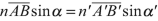
we obtain the Lagrange–Helmholtz relation:

((3.7))

The Lagrange–Helmholtz relation is important and expresses the fact that the quantity $n\kern0.3em y\kern0.3em \alpha$ or paraxial invariant remains constant when light passes through any refracting surface. The formula gives the relationship between transverse magnification, angular magnification, and axial magnification.

Fig. 3.2

Refraction at a single spherical surface and Lagrange–Helmholtz relation. In the case pictured, $\alpha$ and ${\alpha}^{\prime }$ have opposite signs, so the transverse magnification is negative

Centered System

A centered system is a succession of refractive surfaces that have the same axis. Their centers are all situated on the same straight line which is the axis of revolution of the system. For each refractive surface the image serves as the object of the following refractive surface. Each refractive surface establishes a homographic conjugation between the object and its image.

Principal Points and Focal Lengths

An incident ray parallel to the axis (Fig. 3.3) is refracted so as to pass through the image focal point ${F}^{\prime }$. Point ${P}^{\prime }$ is the intersection of this incident ray and of the refracted ray. The plane tangent to the point ${P}^{\prime }$ is called the image principal plane. This plane is the locus of all the points ${P}^{\prime }$ of which the orthogonal projection on the axis is the point ${H}^{\prime }$. This intersection point ${H}^{\prime }$ on the axis is the image principal point. The quantity ${f}^{\prime }=\overline{H^{\prime }F^{\prime }}$ is called the image focal length (Fig. 3.3).

Fig. 3.3

Focal points and principal planes

We define in an identical manner the object principal plane. The point P is located at the intersection of an incident ray which goes through the object focal point F and of the ray which refracts at the point ${P}^{\prime }$ parallel to the axis. The plane tangent to the point P is called the object principal plane. This plane is the locus of all the points P of which the orthogonal projection on the axis is the point H. This intersection H on the axis is the object principal point. The quantity $f=\overline{HF}$ is called the object focal length (Fig. 3.3).

Given an object $\overline{FG}$, the incident ray $\overline{GH}$ which intersects the axis at the point H makes with the axis the angle $\alpha$. This ray $\overline{GH}$ emerges at the point ${H}^{\prime }$ making an angle ${\alpha}^{\prime }$ with the axis. The incident ray $\overline{GH}$, parallel to the axis, which intersects the principal image plane at ${K}^{\prime }$, emerges at the point ${K}^{\prime }$ along $\overline{K^{\prime }F^{\prime }}$ making an angle ${\alpha}^{\prime }$ with the axis (Fig. 3.4). Applying the Lagrange–Helmholtz relation (3.7) and noting that $\overline{FG}=\overline{H^{\prime }K^{\prime }}$ or $y={y}^{\prime }$, we obtain

((3.8))

Moreover as

$$ \alpha =\frac{\overline{FG}}{f},\kern2em \mathrm{and}\kern2.3em {\alpha}^{\prime }=\frac{\overline{H^{\prime }K^{\prime }}}{f^{\prime }},\kern2em \mathrm{we}\ \mathrm{get}\kern2.3em n\frac{\overline{FG}}{f}={n}^{\prime}\frac{\overline{H^{\prime }K^{\prime }}}{f^{\prime }}, $$

and we obtain

((3.9))

The object and image focal lenghts are always of the opposite sign.

Fig. 3.4

Focal lengths

Nodal Points

The object nodal point N and the image nodal point ${N}^{\prime }$ are cardinal points located on the axis. They are such that each incident ray that passes through the object nodal point N emerges from the image nodal point ${N}^{\prime }$ as a ray parallel to the incident ray. This output ray has the same direction as the input ray with a parallel offset (Fig. 3.5). So the incident ray going through N and emerging at ${N}^{\prime }$ forms with the axis the same angles $\alpha$.

Fig. 3.5

Nodal points

Let us take a point G on the object focal plane. An incident ray going through G and parallel to the axis emerges at a point ${P}^{\prime }$ and then through the image point ${F}^{\prime }$ with a direction parallel to an incident ray going through G and the nodal point N.

The triangles GFN and ${P}^{\prime }{H}^{\prime }{F}^{\prime }$ are equal and ${RNN}^{\prime }{R}^{\prime }$ is a parallelogram, and therefore

$$ \overline{FN}=\overline{H^{\prime }F^{\prime }}={f}^{\prime },\kern2em \overline{F^{\prime }N^{\prime }}=\overline{HF}=f,\kern2em \overline{NH}=\overline{N^{\prime }H^{\prime }},\kern2em \overline{NN^{\prime }}=\overline{HH^{\prime }}. $$

In the frequently encountered situation where the refractive index is the same in front of and behind the optical system, the nodal points coincide with the principal points. In a spherical refractive surface, the distance ${HH}^{\prime }$ between the two principal points is nil and both object and image nodal points are coincident with the center of the spherical refractive surface.

Relation of Conjugation and Transverse Magnification

Knowledge of the focal points and of the focal lengths completely determines the system. The principal points and nodal points result immediately from it. The abscissas of any two conjugate points and the magnification can be put in various forms, all of which are various cases of the general homographic relation.

• 1. Origin at the focal points

  Let $\zeta$ be the abscissa of the object point A when we place the origin at the object focal point F, $\overline{FA}=\zeta$. Let ${\zeta}^{\prime }$ be the abscissa of the image point A${}^{\prime }$ measured from the image focal point F${}^{\prime }$, $\overline{F^{\prime }A^{\prime }}={\zeta}^{\prime }$. Moreover $\overline{HF}=f$, $\overline{H^{\prime }F^{\prime }}={f}^{\prime }$, $\overline{AB}=y$, and $\overline{A^{\prime }B^{\prime }}={y}^{\prime }$.

  The triangles ABF and HSF are similar as well as the triangles ${A}^{\prime }{B}^{\prime }{F}^{\prime }$ and ${H}^{\prime }{TF}^{\prime }$. The ratio of their sides is therefore equal. Figure 3.6 can also be used to show that $\overline{AB}=\overline{H^{\prime }T}$ and $\overline{A^{\prime }B^{\prime }}=\overline{HS}$

  $$ -\frac{\overline{HS}}{\overline{AB}}=-\frac{\overline{A^{\prime }B^{\prime }}}{\overline{AB}}=-\frac{\overline{FH}}{\overline{FA}}\kern2em \mathrm{or}\kern2.3em \frac{y^{\prime }}{y}=-\frac{f}{\zeta }, $$

  Fig. 3.6

  

  Relation of conjugation, $\overline{AB}=y$ and $\overline{A^{\prime }B^{\prime }}={y}^{\prime }$

  $$ -\frac{\overline{A^{\prime }B^{\prime }}}{\overline{H^{\prime }T}}=-\frac{\overline{A^{\prime }B^{\prime }}}{\overline{AB}}=-\frac{\overline{F^{\prime }A^{\prime }}}{\overline{F^{\prime }H^{\prime }}}\kern2em \mathrm{or}\kern2.3em \frac{y^{\prime }}{y}=-\frac{\zeta^{\prime }}{f^{\prime }}. $$

  The transverse magnification is

  

  ((3.10))

  Thus we obtain Newton’s conjugation relation:

  

  ((3.11))

  Positive and negative values of $y\slash {y}^{\prime }$ characterize, respectively, an erect or an inverted image, relative to the object.

• 2. Origin at the principal points

  Let $x=\overline{HA}=f+\zeta$ and ${x}^{\prime }=\overline{H^{\prime }A^{\prime }}={f}^{\prime }+{\zeta}^{\prime }$. By replacing in the Newton relation (3–11) $\zeta$ by $x-f$ and ${\zeta}^{\prime }$ by ${x}^{\prime }-{f}^{\prime }$, we get

  $$ {fx}^{\prime }+{f}^{\prime }x={xx}^{\prime }, $$

  and dividing by ${xx}^{\prime }$, we obtain

  

  ((3.12))

  or

  $$ \frac{f}{f^{\prime }}=-\frac{n}{n^{\prime }}, $$
  $$ D=-\frac{n}{f}=\frac{n^{\prime }}{f^{\prime }}. $$

  The conjugation relation is

  

  ((3.13))

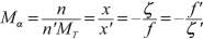
  The transverse magnification is obtained using the Lagrange–Helmholtz relation (3–7)

  $$ ny\alpha ={n}^{\prime }{y}^{\prime }{\alpha}^{\prime }. $$

  The transverse magnification is

  

  ((3.14))

Dioptric Power

The dioptric power is defined by

((3.15))

A positive or convergent system (positive D) thus possesses a negative object focal length and a positive image focal length. For a negative or divergent system (negative D), the object focal length is positive and the image focal length is negative. Instead of power, in the optics books “D” is called “V ” or “vergence,” but this term has another meaning in binocular vision, and thus, in ophthalmology, it is better to use the term of “dioptric power.”

Magnification

In optics, the magnification $\gamma$ is the ratio of the size of an image to the size of the object creating it. There are four types of magnification: the transverse magnification (also called linear or lateral), the angular magnification, the longitudinal magnification, and the pupillary magnification (Fig. 3.7 and Table 3.1).

Fig. 3.7

Magnification

Table 3.1 Magnification

• 1. Transverse magnification has been described above.

  If the origins of the optical system are at the focal points, transverse magnification ${M}_T$ is

  

  ((3.16))

  If the origins of the optical system are at the principal points, transverse magnification ${M}_T$ is

  

  ((3.17))

• 2. Angular magnification

  The Abbe sine condition in mathematical terms is

  

  ((3.18))

  Introducing the transverse magnification ${M}_T$ in the Abbe sine equation,

  $$ \frac{\sin \alpha }{\sin {\alpha}^{\prime }}=\frac{n^{\prime }}{n}{M}_T. $$

  In the Gaussian approximation the angles are small and we get the angular magnification ${M}_{\alpha }$:

  

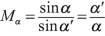  ((3.19))

  From the two previous equations, we get the Lagrange–Helmholtz relation:

  

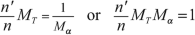  ((3.20))

  so

  

  ((3.21))

• 3. Longitudinal magnification

  The Herschell condition in mathematical terms is

  

  ((3.22))

  Introducing the longitudinal magnification ${M}_L$,

  

  ((3.23))

  The Herschell condition is written as

  $$ \frac{\sin^2\frac{\alpha }{2}}{\sin^2\frac{\alpha^{\prime }}{2}}=\frac{n^{\prime }}{n}{M}_L. $$

  In the Gaussian approximation the angles are small and we get

  $$ \frac{\sin^2\frac{\alpha }{2}}{\sin^2\frac{\alpha^{\prime }}{2}}={\left(\frac{\alpha }{\alpha^{\prime }}\right)}^2=\frac{n^{\prime }}{n}{M}_L={\left(\frac{n^{\prime }}{n}\right)}^2{M}_T^2. $$

  Let the longitudinal magnification ${M}_L$ be

  

  ((3.24))

• 4. The pupillary magnification is the ratio of the diameter of the entrance pupil to the diameter of the exit pupil.

Combination of Two Systems

Let there be a first centered system with object and image principal points ${H}_1$and ${H}_1^{\prime }$, with refractive indices (object and image) ${n}_1$ and ${n}_1^{\prime }$, with object and image focal points ${F}_1$ and ${F}_1^{\prime }$, with object and image focal lengths ${f}_1=\overline{H_1{F}_1}$ and ${f}_1^{\prime }=\overline{H_1^{\prime }{F}_1^{\prime }}$, and with power ${D}_1$.

Let there be likewise a second centered system with object and image principal points ${H}_2$ and ${H}_2^{\prime }$, with refractive indices (object and image) ${n}_2$ and ${n}_2^{\prime }$, with object and image focal points ${F}_2$ and ${F}_2^{\prime }$, with object and image focal lengths ${f}_2=\overline{H_2{F}_2}$ and ${f}_2^{\prime }=\overline{H_2^{\prime }{F}_2^{\prime }}$, and with power ${D}_2$.

The two systems are placed end to end, on a common axis with the same medium between the two systems, so ${n}_1^{\prime }={n}_2$. The combination of the two systems has for object index $n={n}_1$ and for image index ${n}^{\prime }={n}_2^{\prime }$. Optics Interval is defined by $\Delta =\overline{F_1^{\prime }{F}_2}$ (Fig 3.8).

Fig. 3.8

Compound thick lens

• (a) Determination of the object focal point

  If we need to get an emerging ray of the second system which emerges parallel to the axis, the incident ray of the second system must go through the object focal point ${F}_2$. The object focal point F of the combination of the two systems will be defined as being the object having the image ${F}_2$ through the first system. Applying Newton’s formula to the first system, we get

  $$ \overline{F_1F}\kern2.77695pt \overline{F_1^{\prime }{F}_2}={f}_1{f}_1^{\prime }. $$

  (3.25)

  The position of the object focal point F of the combination of the two systems is

  

  ((3.26))

• (b) Determination of the image focal point

  An incident ray on the first system, parallel to the axis, emerges from the first system going through the image focal point ${F}_1^{\prime }$. The image focal point ${F}^{\prime }$ of the combination of the two systems is none other than the image of ${F}_1^{\prime }$ through the second system. Applying Newton’s formula to the second system, we get

  $$ \overline{F_2{F}_1^{\prime }}\kern2.77695pt \overline{F_2^{\prime }F^{\prime }}={f}_2\kern2.77695pt {f}_2^{\prime }. $$

  (3.27)

  The position of the image focal point ${F}^{\prime }$ of the combination of the two systems is

  

  ((3.28))

• (c) Determination of the object focal length

  The object principal plane is the locus of all the K points of which the projection on the axis is the image principal point H. Applying the Thales theorem which says that if a straight line is drawn parallel to a side of a triangle, then it divides the other two sides proportionally (Fig. 3.8):

  $$ \frac{\overline{FH}}{\overline{F{H}_1}}=\frac{\overline{HK}}{\overline{H_1{I}_1}}=\frac{\overline{H_2{I}_2}}{\overline{H_1^{\prime }{I}_1^{\prime }}}=\frac{\overline{F_2{H}_2}}{\overline{F_2{H}_1^{\prime }}}, $$

  hether

  $$ \frac{\overline{HF}}{\overline{H_1{F}_1}+\overline{F_1F}}=\frac{f}{f_1+\frac{f_1{f}_1^{\prime }}{\Delta}}=\frac{\overline{H_2{F}_2}}{\overline{H_1^{\prime }{F}_1^{\prime }}+\overline{F_1^{\prime }{F}_2}}=\frac{f_2}{f_1^{\prime }+\Delta}. $$

  The object focal length is

  

  ((3.29))

• (d) Determination of the image focal length

  The image principal plane is the locus of all the ${K}^{\prime }$ points of which the projection on the axis is the image principal point ${H}^{\prime }$. Applying the Thales theorem (Fig. 3.8),

  $$ \frac{\overline{F^{\prime }H^{\prime }}}{\overline{F^{\prime }{H}_2^{\prime }}}=\frac{\overline{H^{\prime }K^{\prime }}}{\overline{H_2^{\prime }{I}_2^{\prime }}}=\frac{\overline{H_1^{\prime }{I}_1^{\prime }}}{\overline{H_2{I}_2}}=\frac{\overline{F_1^{\prime }{H}_1^{\prime }}}{\overline{F_1^{\prime }{H}_2^{\prime }}}, $$

  hether

  $$ \frac{\overline{H^{\prime }F^{\prime }}}{\overline{H_2^{\prime }{F}_2^{\prime }}+\overline{F_2^{\prime }F^{\prime }}}=\frac{f^{\prime }}{f_2^{\prime }+\frac{f_2{f}_2^{\prime }}{\Delta}}=\frac{\overline{H_1^{\prime }{F}_1^{\prime }}}{\overline{H_2{F}_2}+\overline{F_2{F}_1^{\prime }}}=\frac{f_1^{\prime }}{f_2-\Delta}. $$

  The image focal length is

  

  ((3.30))

  Through the combination of two systems, ${F}_1$ and ${F}_2^{\prime }$ are conjugated. Furthermore wet get these other relations:

  $$ \frac{f_1^{\prime }}{f_1}=-\frac{n_1^{\prime }}{n}\kern0.3em \mathrm{and}\kern0.3em \frac{f_2^{\prime }}{f_2}=-\frac{n^{\prime }}{n_2}, $$
  

  ((3.31))

• (e) Determination of dioptric power for a compound of two systems

  The dioptric power or vergence of each system is given by

  $$ {D}_1=-\frac{n_1}{f_1}=\frac{n}{f_1^{\prime }}, $$

  (3.32)
  $$ {D}_2=-\frac{n}{f_2}=\frac{n_2}{f_2^{\prime }}, $$

  (3.33)

  and the power of the two systems is given by

  $$ D=-\frac{n_1}{f}=\frac{n_2}{f^{\prime }}=-\frac{n_2.\Delta}{f_1^{\prime }{f}_2^{\prime }}. $$

  (3.34)

  The optics interval can be break down as

  $$ \Delta =\overline{F_1^{\prime }{F}_2}=\overline{F_1^{\prime }{H}_1^{\prime }}+\overline{H_1^{\prime }{H}_2}\overline{H_1^{\prime }{H}_2}+\overline{H_2{F}_2}=-{f}_1^{\prime }+{f}_2+\overline{H_1^{\prime }{H}_2}, $$

  hence

  $$ {\displaystyle \begin{array}{rlll}D& =-\frac{-{n}_2{f}_1^{\prime }+{n}_2{f}_2+{n}_2\overline{H_1^{\prime }{H}_2}}{f_1^{\prime }{f}_2^{\prime }},& & \\ {}D& =\frac{n_2}{f_2^{\prime }}-\frac{n}{f_1^{\prime }}\frac{n_2}{f_2^{\prime }}\frac{f_2}{n}-\frac{n}{f_1^{\prime }}\frac{n_2}{f_2^{\prime }}\frac{\overline{H_1^{\prime }{H}_2}}{n},& & \\ {}D& ={D}_2+\left({D}_1{D}_2\frac{1}{D_2}\right)-{D}_1{D}_2\overline{H_1^{\prime }{H}_2},& & \end{array}} $$

  and we get the Gullstrand relation:

  

  ((3.35))

Single Lens

After the refracting surface where there is only one interface, the simplest centered system is the lens. The lens has two spherical refractive surfaces. The cornea is a meniscus lens, and the crystalline lens is biconvex. For the first refractive surface, the refractive indices of the object and image media are ${n}_1$ and ${n}_1^{\prime }$, and the radius of curvature is ${r}_1$.

((3.36))

For the second refractive surface, the refractives indices of the object and image media are ${n}_2$ and ${n}_2^{\prime }$, and the radius of curvature is ${r}_2$.

((3.37))

If the lens of index n is placed in a medium with an index ${n}_0$, we have $n={n}_1^{\prime }={n}_2$ and ${n}_0={n}_1={n}_2^{\prime }$. If the lens thickness on the optical axis is t, and according to the formula of combination, we get the power of the lens

((3.38))

For a biconvex lens with radii ${r}_1$ and ${r}_2$ and diameter d, the thickness of the lens t is calculated with the formula of coupola (Figs. 3.9, 3.10). The height of each coupola of the lens is ${h}_1$ and ${h}_2$, and the thickness at the border of the lens is ${t}_0$. The thickness of the lens is $t={h}_1+{t}_0+{h}_2$ with

((3.39))

Fig. 3.9

Biconvex lens

Fig. 3.10

Design of a biconvex lens

Entrance and Exit Pupils

The pupil is the surface limited by the inner border of the iris. The pupil of the human eye acts as the aperture stop of the eye. When the real pupil is seen from outside, an observer sees the entrance pupil which is a virtual image of the real pupil as seen through the corneal refraction. In the example below, entrance and exit pupils of the human eye are calculated with the values of Le Grand’s theoretical eye.

• 1. The entrance pupil ${\Delta}_0$ is conjugated to the real pupil $\Delta$ in the object space when the light beam goes through the sub-optical system which is anterior to the pupil (cornea). In this example we calculate the position and the diameter of the entrance pupil of the theoretical eye. We assume that the anterior surface of the iris is in a frontal plane tangent to the cristalline lens apex. The pupil is at the distance of $3.60\kern0.3em \mathrm{mm}$ from the corneal apex S. The position of the principal planes of the cornea is at $0.06\kern0.3em \mathrm{mm}$ in front of the cornea. Thus the real pupil is at the distance of $3.60+0.06=3.66\kern0.3em \mathrm{mm}$ from the image principal plane of the cornea. The refractive index of aqueous humor is 1.3374 and the corneal power is ${D}_c$. According to the equation of conjugation (3.1):

  $$ \frac{n^{\prime }}{x^{\prime }}=\frac{n}{x}+\frac{n^{\prime }-n}{r}, $$

  we get

  $$ \frac{1}{x}=\frac{n^{\prime }}{x^{\prime }}-{D}_c=\left[1.3374\slash \left(3.66\ast 1{0}^{-3}\right)\right]-42.36=323.05, $$
  $$ x=\frac{1}{323.05}=0.0031\kern0.3em \mathrm{m}, $$

  and $x=3.10\kern0.3em \mathrm{mm}.$

  The distance between the apex of the cornea and the entrance pupil is $3.10-0.06=3.04\kern0.3em \mathrm{mm}$. The entrance pupil is located in front of the real pupil and slightly enlarged. Applying the equation of transverse magnification (3.14), where ${\Delta}_0$ is the size of the entrance pupil and $\Delta$ the diameter of the real pupil:

  $$ {M}_T=\frac{y^{\prime }}{y}=\frac{nx^{\prime }}{n^{\prime }x}\kern1em \mathrm{and}\kern1.3em \frac{\Delta_o}{\Delta}=\frac{n^{\prime }x}{nx^{\prime }}\frac{1.3374}{1}\kern2.77695pt \frac{3.10}{3.66}=1.13, $$

  thus

  $$ {\Delta}_o=\Delta \ast 1.13. $$

  For a real pupil with a $6\kern0.3em \mathrm{mm}$ diameter (scotopic vision), the entrance pupil diameter is $6\ast 1.13=6.78\kern0.3em \mathrm{mm}$, for a real pupil with a $4\kern0.3em \mathrm{mm}$ diameter (mesopic vision), the entrance pupil diameter is $4\ast 1.13=4.52\kern0.3em \mathrm{mm}$, and for a real pupil with a $2\kern0.3em \mathrm{mm}$ diameter (photopic vision), the entrance pupil diameter is $2\ast 1.13=2.26\kern0.3em \mathrm{mm}$.

• 2. The exit pupil ${\Delta}_i$ is conjugated to the real pupil $\Delta$ in the image space when the light beam goes through the sub-optical system which is posterior to the pupil (crystalline lens). In the same way we calculte the position and the diameter of the exit pupil of the theoretical eye. The refractive index of aqueous humor is 1.3374 and the crystalline lens power is ${D}_{cl}$. The pupil is at the distance of $3.60\kern0.3em \mathrm{mm}$ from the vertex. The distance x between the corneal apex and the object principal plane of the crystalline lens is $6.02\kern0.3em \mathrm{mm}$. The distance between the real pupil and the object principal plane of the crystalline lens x is $6.02-3.60=2.42\kern0.3em \mathrm{mm}$. The distance between the image principal plane of the crystalline lens and the image of the real pupil after passing through the crystalline lens is ${x}^{\prime }$. According to the equation of conjugation (3.1):

  $$ \frac{n^{\prime }}{x^{\prime }}=\frac{n}{x}+\frac{n^{\prime }-n}{r}, $$

  we get

  $$ \frac{n^{\prime }}{x^{\prime }}=\frac{n}{x}+{D}_{cl}=-\left[1.3374\slash \left(2.42\ast 1{0}^{-3}\right)\right]+21.78=530.86, $$
  $$ {x}^{\prime }=\frac{1.336}{530,86}=0.00252\kern0.3em m, $$

  and ${x}^{\prime }=2.52\kern0.3em \mathrm{mm}.$

  The distance between the corneal apex and the image principal plane of the crystalline lens is $6.20\kern0.3em \mathrm{mm}$. The distance between the apex of the cornea and the exit pupil is $6.20-2.52=3.68\kern0.3em \mathrm{mm}$.

  The exit pupil is located behind the true pupil and slightly enlarged. Applying the equation of transverse magnification (3.14), where ${\Delta}_i$ is the diameter of the exit pupil and $\Delta$ the diameter of the real pupil, the diameter of the exit pupil ${\Delta}_i$ is obtained as

  $$ {M}_T=\frac{y^{\prime }}{y}=\frac{nx^{\prime }}{n^{\prime }x}\kern1em \mathrm{and}\kern1.3em \frac{\Delta_i}{\Delta}=\frac{nx^{\prime }}{n^{\prime }x}=\frac{1.3374}{1.336}\kern2.77695pt \frac{2.52}{2.42}=1.04, $$

  thus

  $$ {\Delta}_i=\Delta \ast 1.04. $$

  To calculate the diameter of the exit pupil based on the diameter of the entrance pupil, we have

  $$ \Delta =\frac{\Delta_o}{1.13}\kern1em \mathrm{and}\ \mathrm{we}\ \mathrm{get}\kern1.3em {\Delta}_i=\frac{\Delta_o}{1.13}\ast 1.04, $$

  thus

  $$ {\Delta}_i={\Delta}_o\ast 0.92. $$

  Consequently, the diameter of the exit pupil is equal to the diameter of the entrance pupil multiplied by $0.92$. Thus, for a real pupil with a $6\kern0.3em \mathrm{mm}$ diameter (scotopic vision), the exit pupil diameter is $6.78\ast 0.92=6.24\kern0.3em \mathrm{mm}$, for a real pupil with a $4\kern0.3em \mathrm{mm}$ diameter (mesopic vision), the exit pupil diameter is $4.52\ast 0.92=4.16\kern0.3em \mathrm{mm}$, and for a real pupil with a $2\kern0.3em \mathrm{mm}$ diameter (photopic vision), the exit pupil diameter is $2.26\ast 0.92=2.08\kern0.3em \mathrm{mm}$.

  The pupil magnification is the ratio of the diameter of the exit pupil to the diameter of the entrance pupil (Fig. 3.11):

  $$ {M}_P=\frac{\Delta_i}{\Delta_o}. $$

  Fig. 3.11

  

  Entrance and exit pupils of the eye. AB (${\Delta}_o$) is the entrance pupil, and ${A}^{\prime }{B}^{\prime }$ (${\Delta}_i$) is the exit pupil

Matrix Method in Paraxial Optics

The matrix method provides an alternative way for solving paraxial optics problems. Matrices are a mathematical tool designed to deal with linear equations, so that it is natural to apply matrices to paraxial ray tracing. The matrix method will be used to find the first-order properties of the schematic eye and to calculate its cardinal elements.

Elementary Matrices

(a) Vergence of a Spherical Surface

By definition, the vergence or dioptric power of a spherical surface, which separates two media with indices ${n}_1$ and ${n}_2$, is

$$ V\equiv \frac{n_2-{n}_1}{\overline{R}}, $$

where $\overline{R}\equiv \overline{SC}$ is the radius of curvature in algebraical value of which the sign is linked to the direction of the incident light. When R is expressed in meter, the unity for the vergence is the diopter $\delta$

(b) Refraction Matrix

In the Gaussian approximation, the linearity of the equations of crossing a spherical surface suggests to use the matrix calculation. The column matrix is defined with the first element $\underline{X}$ which is the position $\underline{x}$ of the crossing point of the ray with the interface and the second element $n\underline{\alpha}$ or optical angle which is the product of the index by the tilt angle of the ray with the optical axis:

$$ \underline{X}\equiv \left[\begin{array}{l}\hfill \underline{x}\hfill \\ {}\hfill n\underline{\alpha}\hfill \end{array}\right]. $$

The crossing of a spherical surface is written as

$$ {\left[\begin{array}{l}\hfill \underline{x}\hfill \\ {}\hfill n\underline{\alpha}\hfill \end{array}\right]}_2=\left[\begin{array}{ll}\hfill 1\hfill & \hfill 0\hfill \\ {}\hfill -V\hfill & \hfill 1\hfill \end{array}\right]{\left[\begin{array}{l}\hfill \underline{x}\hfill \\ {}\hfill n\underline{\alpha}\hfill \end{array}\right]}_1 $$

in a condensed form, ${\underline{X}}_2=\mathbb{R}(S){\underline{X}}_1$, where

is the refraction matrix of the spherical surface.

The value of the determinant of $\mathbb{R}(S)$ is 1: det $\mathbb{R}=1$.

(c) Translation Matrix

The translation matrix is the transformation matrix of the column matrix X between two frontal planes ${A}_1 xy$ and ${A}_2 xy$ located in the same homogeneous medium. Using the complex notation and introducing the index, the equations of transformation are

$$ {\underline{x}}_2={\underline{x}}_1+\frac{\overline{A_1{A}_2}}{n}{\left(n\underline{\alpha}\right)}_1\kern2em \mathrm{and}\kern2em {\left(n\underline{\alpha}\right)}_2={\left(n\underline{\alpha}\right)}_1. $$

Matrix-wise, this is written as

$$ {\left[\begin{array}{l}\hfill \underline{x}\hfill \\ {}\hfill n\underline{\alpha}\hfill \end{array}\right]}_2=\left[\begin{array}{ll}\hfill 1\hfill & \hfill \overline{A_1{A}_2}\slash n\hfill \\ {}\hfill 0\hfill & \hfill 1\hfill \end{array}\right]{\left[\begin{array}{l}\hfill \underline{x}\hfill \\ {}\hfill n\underline{\alpha}\hfill \end{array}\right]}_1. $$

In a condensed form, ${\underline{X}}_2=\mathcal{T}\left(\overline{A_1{A}_2}\right){\underline{X}}_1$ with

The effective length that characterizes the translation matrix is the reduced length $\overline{A_1{A}_2}\slash n$. The value of the determinant of $\mathcal{T}\left(\overline{A_1{A}_2}\right)$ is 1: det $\mathcal{T}\left(\overline{A_1{A}_2}\right)=1$.

Centered Systems

A centered system is composed of many refractive or reflective surfaces, usually spherical, such that the set has a symmetry around the same axis of Oz. The centered optical systems, composed of a series of homogeneous media, separated by spherical interfaces, are characterized in the Gaussian approximation by a linear relationship. Two methods are used to get the image of an object. The first is algebraical, and it is based on the conjugate relationships between the positions of the objects and the corresponding images. The second is geometrical, and it visualizes the particular rays of light.

(a) Transfer Matrix of a Centered System

Let us consider a centered system made up of p refractive spherical surfaces separated by homogeneous media.E is the first interface and S is the last interface of the system. Let $T\left(\overline{ES}\right)$ be the transfer matrix of the system. The parameters that define the ray of light in all the frontal plane are the following complex numbers: the abscissa $\underline{x}=x+ iy$ and the optical angle $\underline{\alpha}=n\left(\alpha + i\beta \right)$. Therefore the entrance and exit matrices are written as

$$ {\underline{X}}_e={\left[\begin{array}{l}\hfill \underline{x}\hfill \\ {}\hfill n\underline{\alpha}\hfill \end{array}\right]}_e\kern2em \mathrm{and}\kern2em {\underline{X}}_s={\left[\begin{array}{l}\hfill \underline{x}\hfill \\ {}\hfill n\underline{\alpha}\hfill \end{array}\right]}_s. $$

The product of elementary matrices of translation $\mathcal{T}$ and of refraction $\mathbb{R}$, writen from right to left following the succession of the spherical surfaces crossed by light, is a matrix $T\left(\overline{ES}\right)$ with four elements. By definition

$$ T\left(\overline{ES}\right)\equiv \mathcal{T}\left(\overline{S_pS}\right)\mathbb{R}\left({S}_p\right)\cdots \mathcal{T}\left(\overline{S_1{S}_2}\right)\mathbb{R}\left({S}_1\right)\mathcal{T}\left(\overline{E{S}_1}\right) $$

is the transfer matrix of the centered system. It is written as

$$ T\left(\overline{ES}\right)=\left[\begin{array}{ll}\hfill a\hfill & \hfill b\hfill \\ {}\hfill c\hfill & \hfill d\hfill \end{array}\right]. $$

The relationship ${\underline{X}}_s=T\left(\overline{ES}\right){\underline{X}}_e$ is explained as follows:

$$ {\underline{X}}_s=a{\underline{x}}_e+b{\left(n\underline{\alpha}\right)}_e\kern2em \mathrm{and}\kern2em {\left(n\underline{\alpha}\right)}_s=c{\underline{x}}_e+d{\left(n\underline{\alpha}\right)}_e. $$

The four elements $a,b,c$, and d, callled Gaussian constants, are linked by a relationship because the determinant of $T\left(\overline{ES}\right)$, the product of matrices of determinants equal to 1, is also equal to 1.

(b) Vergence of a Centered System

The transfer matrix $T\left(\overline{A_1{A}_2}\right)$ between two frontal planes ${A}_1 xy$ and ${A}_2 xy$, respectively, located in the object space and in the image space, with the indices ${n}_o$ and ${n}_i$, is expressed as

$$ T\left(\overline{A_1{A}_2}\right)=\mathcal{T}\left(\overline{S{A}_2}\right)T\left(\overline{ES}\right)\mathcal{T}\left(\overline{A_1E}\right). $$

This matrix transfer of the total system which takes a ray from the object to the image is named conjugate matrix. For the couple of points ${A}_1$ and ${A}_2$, with ${z}_1\equiv \overline{E{A}_1}$ and ${z}_2\equiv \overline{S{A}_2}$ and with ${T}_{ij}(A)$ the elements of the conjugate matrix, the previous relationship is written as

$$ \left[\begin{array}{ll}\hfill {T}_{11}(A)\hfill & \hfill {T}_{12}(A)\hfill \\ {}\hfill {T}_{21}(A)\hfill & \hfill {T}_{22}(A)\hfill \end{array}\right]=\left[\begin{array}{ll}\hfill 1\hfill & \hfill {z}_2\slash {n}_i\hfill \\ {}\hfill 0\hfill & \hfill 1\hfill \end{array}\right]\left[\begin{array}{ll}\hfill a\hfill & \hfill b\hfill \\ {}\hfill c\hfill & \hfill d\hfill \end{array}\right]\left[\begin{array}{ll}\hfill 1\hfill & \hfill -{z}_1\slash {n}_o\hfill \\ {}\hfill 0\hfill & \hfill 1\hfill \end{array}\right], $$

which gives in performing and in identifying

$$ {\displaystyle \begin{array}{rlllllll}{T}_{11}(A)& =a+c\frac{z_2}{n_i}& \kern2em {T}_{12}(A)& =-a\frac{z_1}{n_o}+b+\frac{z_2}{n_i}\left(-c\frac{z_1}{n_o}+d\right)& & & & \\ {}{T}_{21}(A)& =c& \kern2em {T}_{22}(A)& =d-c\frac{z_1}{n_o}.& & & & \end{array}} $$

By definition the vergence of a system is the opposite of c:

$$ V\equiv -c. $$

Matrix-wise, we write

$$ {\left[\begin{array}{l}\hfill \underline{x}\hfill \\ {}\hfill n\underline{\alpha}\hfill \end{array}\right]}_s=\left[\begin{array}{ll}\hfill a\hfill & \hfill b\hfill \\ {}\hfill -V\hfill & \hfill d\hfill \end{array}\right]{\left[\begin{array}{l}\hfill x\hfill \\ {}\hfill 0\hfill \end{array}\right]}_e, $$

or in a condensed form, ${\underline{X}}_s=T\left(\overline{ES}\right){\underline{X}}_e$, from where ${n}_i{\alpha}_s=-V{x}_e$.

If $V>0$, the system is converging. If $V<0$, the system is diverging. If $V=0$, the system is afocal.

(c) Conjugate Matrix

Let us consider a centered system and two conjugates planes which are perpendicular to the optical axis and which contain the points ${A}_o,{A}_i,{B}_o$ and ${B}_i$. We write ${z}_o\equiv \overline{E{A}_o}$ and ${z}_i\equiv \overline{S{A}_i}$ Each element of the transfer matrix of the system between these two conjugate planes or a conjugate matrix is written as

$$ {\displaystyle \begin{array}{rlllllll}{T}_{11}(A)& =a-V\frac{z_i}{n_i}& \kern2em {T}_{12}(A)& =-a\frac{z_o}{n_o}+b+\frac{z_i}{n_i}\left(V\frac{z_o}{n_o}+d\right)& & & & \\ {}{T}_{21}(A)& =-V& \kern2em {T}_{22}(A)& =d+V\frac{z_o}{n_o}.& & & & \end{array}} $$

Explaining the matrix relationship ${\underline{X}}_i=T\left(\overline{A_o{A}_i}\right){\underline{X}}_o$, it becomes

$$ {\underline{x}}_i={T}_{11}(A){\underline{x}}_o+{T}_{12}(A){n}_o{\underline{\alpha}}_o\kern2em \mathrm{and}\kern2em {n}_i{\underline{\alpha}}_i=-V{\underline{x}}_o+{T}_{22}(A){n}_o{\underline{\alpha}}_o. $$

As the position ${\underline{x}}_i$ of the image ${B}_i$ is independent of the tilt ${\underline{\alpha}}_o$ of the rays coming from ${A}_o$, we obtain the conjugate relationship which is given ${T}_{12}(A)\equiv 0$ and let

The transverse magnification ${M}_t$, in the case of the Gaussian approximation, is given by the formula:

$$ {M}_t=\frac{\overline{A_i{B}_i}}{\overline{A_o{B}_o}}. $$

${T}_{11}(A)$ is identified to the transverse magnification ${M}_t$.

The angular magnification is defined by ${M}_a\equiv {\left({\underline{\alpha}}_i\slash {\underline{\alpha}}_o\right)}_{x_o}=0$.

${T}_{22}(A)$ is worth:

$$ {T}_{22}(A)={\left(\frac{n_i{\alpha}_i}{n_o{\alpha}_o}\right)}_{x_o=0}=0, $$

$$ {T}_{22}(A)=\frac{n_i}{n_o}{M}_a. $$

The transfer matrix between two conjugate planes is written as

The determinant of $T\left(\overline{A_o{A}_i}\right)$ being equal to 1, we get the Lagrange and Helmholtz relation:

Which is also written as

$$ {n}_o{x}_o{\alpha}_o={n}_i{x}_i{\alpha}_i. $$

(d) Homographic Relation

By definition a homographic function is represented in the form of a quotient of affine functions which can be written as

$$ y=\frac{ax+b}{cx+ dx}. $$

This function determines a bijection if $\left( ad- bc\right)\ne 0$ Every object point and its image point form a conjugate pair, and by the principle of inverse return of the light, the pair persists when the image becomes object and vice versa. This relation is easily obtained with the help of the matrices $T\left(\overline{ES}\right)$ and $T\left(\overline{A_o{A}_i}\right)$. With the usual notations (${z}_o=\overline{E{A}_o}$, ${z}_i=\overline{S{A}_i}$, etc.), as ${A}_o$ and ${A}_i$ are conjugated, we get

It results the following homographic relation:

Cardinal Elements

In the Gaussian optics or paraxial approximation, the cardinal elements are sufficient to calculate the position and the size of the image of an object. These elements are the focal lengths (and the focal planes), the principal planes, and the nodal points (Fig. 3.12).

Fig. 3.12

Cardinal elements

 

• (a) Focal lengths

  By definition, the image and object focal lengths are the following algebraical quantities:

  

  If $V>0,{f}_i>0$ and ${f}_o<0$ On the other side, if $V<0,{f}_i<0$ and ${f}_o>0$ If the extreme media are identical, ${f}_i=-{f}_o$

• (b) Principal planes

  Principal planes are frontal conjugate planes ${H}_o xy$ and ${H}_i xy$ such that the transverse magnification ${M}_t$ is equal to unity. It results that the transfer matrix $T\left(\overline{H_o{H}_i}\right)$ between the principal planes has for expression

  $$ T\left(\overline{H_o{H}_i}\right)=\left[\begin{array}{ll}\hfill 1\hfill & \hfill 0\hfill \\ {}\hfill -V\hfill & \hfill 1\hfill \end{array}\right], $$

  and we can write

  $$ {T}_{11}(H)=1=a-V\frac{\overline{S{H}_i}}{n_i}\kern2em \mathrm{and}\kern2em {T}_{22}(H)=1=d+V\frac{\overline{E{H}_o}}{n_o}. $$

  Therefore, the positions of the principal planes of a centered system, in function of the transfer matrix $T\left(\overline{ES}\right)$ of this system, are given by the relations:

  

• (c) Nodal points

  The two nodal points, ${N}_o$ and ${N}_i$, are two conjugate points located on the optical axis such that all incident rays going through ${N}_o$ emerge from ${N}_i$ in parallel to its incident direction. Therefore

  

  The transfer matrix $T\left(\overline{N_o{N}_i}\right)$ is written as

  $$ T\left(\overline{N_o{N}_i}\right)=\left[\begin{array}{ll}\hfill {n}_o\slash {n}_i\hfill & \hfill 0\hfill \\ {}\hfill -V\hfill & \hfill {n}_i\slash {n}_o\hfill \end{array}\right]. $$

  From where the following relationships,

  $$ {T}_{11}(N)=\frac{n_o}{n_i}=a-V\frac{\overline{S{N}_1}}{n_i}\kern2em \mathrm{and}\kern2em {T}_{22}(N)=\frac{n_i}{n_o}=d+V\frac{\overline{E{N}_o}}{n_o} $$

  and the positions of these points from E and S:

  

  similarly from the principal planes ${H}_i$ and ${H}_o$,

  

  Thus the distances $\overline{H_o{H}_i}$ and $\overline{N_o{N}_i}$ are equal.

• (d) Focal planes

  These frontal planes in the object space and in the image space are written as ${F}_o xy$ and ${F}_i xy$ and are defined as follows:

  All the incident rays of light, coming from ${F}_o$, emerge parallel to the optical axis.

  All the incident rays of light, parallel to the optical axis, emerge converging to ${F}_i$.

  Object focal point ${\mathbf{F}}_{\mathbf{o}}$

  To locate ${F}_o$, the relationship between the entrance and exit parameters is written as

  $$ {x}_s=a{x}_e+b{n}_o{\alpha}_e\kern2em \mathrm{and}\kern2em {n}_i{\alpha}_s=-V{x}_e+d{n}_o{\alpha}_e. $$

  As ${\alpha}_s=0$ whatever ${x}_e$ and ${\alpha}_e$ it becomes

  $$ \frac{x_e}{\alpha_e}=\frac{n_o}{V}d. $$

  So, the incident rays of light come from a point ${F}_o$ such that, algebraically,

  $$ -\overline{E{F}_o}=\frac{x_e}{\alpha_e}=\frac{n_o}{V}d. $$

  It results

  

  Image focal point ${\mathbf{F}}_{\mathbf{i}}$

  As in this case ${\alpha}_e=0$ whatever ${x}_s$ and ${\alpha}_s$ it becomes

  $$ {x}_s=a{x}_e\kern2em \mathrm{and}\kern2em {n}_i{\alpha}_s=-V{x}_e, $$

  hence

  $$ \frac{x_s}{\alpha_s}=-{n}_i\frac{a}{V}. $$

  So, the rays of light emerge at the point ${F}_i$ such that, algebraically,

  $$ -\overline{S{F}_i}=-\frac{x_s}{\alpha_s}=\frac{n_i}{V}a. $$

  It results:

  

  In summary, the cardinal elements calculated with the Gaussian constants $a,b,-V$, and d of the transfer matrix $\left[\begin{array}{ll}\hfill a\hfill & \hfill b\hfill \\ {}\hfill -V\hfill & \hfill d\hfill \end{array}\right]$ of a centered system are

  $$ {\displaystyle \begin{array}{rlll}\mathrm{object}\ \mathrm{focal}\ \mathrm{length}:\kern10em {f}_o& =-\frac{n_o}{V}& & \\ {}\mathrm{image}\ \mathrm{focal}\ \mathrm{length}:\kern10.3em {f}_i& =\frac{n_i}{V}& & \\ {}\mathrm{position}\ \mathrm{of}\ \mathrm{the}\ \mathrm{object}\ \mathrm{principal}\ \mathrm{point}:\kern2em \overline{E{H}_o}& ={f}_o\kern2.77695pt \left(d-1\right)& & \\ {}\mathrm{position}\ \mathrm{of}\ \mathrm{the}\ \mathrm{image}\ \mathrm{principal}\ \mathrm{point}:\kern2em \hspace{2.22198pt}\overline{S{H}_i}& ={f}_i\kern2.77695pt \left(a-1\right)& & \\ {}\mathrm{position}\ \mathrm{of}\ \mathrm{the}\ \mathrm{object}\ \mathrm{focal}\ \mathrm{point}:\kern3em \hspace{4.44pt}\overline{E{F}_o}& =-\frac{n_0}{V}d& & \\ {}\mathrm{position}\ \mathrm{of}\ \mathrm{the}\ \mathrm{image}\ \mathrm{focal}\ \mathrm{point}:\kern3em \hspace{6.66pt}\overline{S{F}_i}& =\frac{n_i}{V}a& & \\ {}\mathrm{position}\ \mathrm{of}\ \mathrm{the}\ \mathrm{object}\ \mathrm{nodal}\ \mathrm{point}:\kern3em \overline{E{N}_o}& ={f}_o\kern2.77695pt \left(d-\frac{n_i}{n_o}\right)& & \\ {}\mathrm{position}\ \mathrm{of}\ \mathrm{the}\ \mathrm{image}\ \mathrm{nodal}\ \mathrm{point}:\kern3.3em \overline{S{N}_i}& ={f}_i\kern2.77695pt \left(a-\frac{n_o}{n_i}\right)& & \\ {}\mathrm{transverse}\ \mathrm{magnification}:\kern7.3em {M}_t& =a& & \\ {}\mathrm{angular}\ \mathrm{magnification}:\kern7.3em \hspace{11.10pt}{M}_a& =\frac{n_o}{n_i}d.& & \end{array}} $$

Limits of Paraxial Approximation for the Eye

Two preliminary questions arise: Is the eye a centered system and can we use the paraxial approximation under normal conditions of vision? Strictly, the eye is not a centered system. The four diopters of the eye, anterior and posterior corneal surfaces and anterior and posterior surfaces of the crystalline lens, are not surfaces of revolution. The eye has at least eight surfaces with discontinuity of indices: two for the cornea (epithelium and cornea) and six for the cristalline lens (nucleus and cortex). The surfaces of the cornea and the cristalline lens are not spherical. The axis of the cristalline lens does not go through the axis of the cornea. This gap can be higher than 0.1 mm which is equivalent to an imprecision of 1${}^{\circ }$ to 2${}^{\circ }$ on the definition of the optical axis.

With a pupil diameter of 4 mm and a mean radius of corneal curvature of 8 mm, the sine of an angle of incidence i of a ray of light parallel to the axis and going through the border of the pupille is $0.25$ or about $i=14.{5}^{\circ }$, that is to say $i=0.253$ rad. There is a difference of more than 1$\%$ between i and $\sin i$.

For the posterior surface of the crystalline lens, the differences between the angles of incidence and their sine are even higher; so all in all a difference of more than 2$\%$ is likely between the paraxial way and the true way of the ray of light. For an ocular vergence of about 60 $\delta$, this 2$\%$ difference is more than one diopter. Strictly speaking, we must study the formation of the images on the retina only in thinking about the true propagation of the ray of light from the corneal vertex to the retina.

Moreover the optical axis, pupil axis, line of sight, and visual axis are not aligned.

Despite that, the paraxial approximation can be used to study the optics of the vision and the corrections of the ametropia with the glasses or with the shaping of the cornea with an excimer laser, because the analysis of the difference between the true ray tracing and the paraxial approximation involves little in the correction. Indeed in first analysing, the paraxial approximation can be used for the eye because on the one hand the cornea flattens from the center to the periphery, and on the other hand the aberrations of the eye are a constant data for the non-corrected eye as for the corrected eye.

However for the intraocular lens correction of cataract surgery, the clinical studies show that the expected results of the formulas using only the paraxial approximation differ from the achieved results with a standard deviation of $\pm$ 1 diopter. These formulas must be adjusted including a correcting factor which is calculated usually with a statistical regression formula.

Schematic Eye

The eye is a complex optical system having a succession of spherical interfaces which are not perfectly spherical, of which media are differents and the index of the cristalline lens is not a constant. The schematic eye is an optical system obtained by taking into account the succession of the four spherical diopters centered on the same axis for which we calculate, in the Gaussian approximation, the cardinal elements and the ocular optical constants. The human theoretical eye is a fictitious eye which represents a mean of the dimensions of the adult eye for which we calculate in the Gaussian approximation the cardinal elements and the ocular optical constants (Fig. 3.13).

Fig. 3.13

Interfaces of the schematic eye

The matrix calculation has been applied to the eye for the first time by Le Grand and Bourdy (Table 3.2). The use of the matrices, applied to Colliac’s theoretical eye, allows to find right away the formulas of association of a combination of optical systems and to calculate the cardinal elements (Fig. 3.14 and Table 3.3).

Fig. 3.14

Principal planes of a schematic eye

Table 3.2 Gaussian elements of the transfer matrix of the eye

Table 3.3 Theoretical eye

For our Colliac’s schematic eye, we get the system matrix of the eye with the four Gaussian constants A, B, C, and D ($\mathrm{C}=-\mathrm{V}$):

The dimensions of the human eye vary from person to person. The mean values of the dimension of an adult eye are indicated in Table 3.2. The crystalline lens index of the crystalline lens is not a constant and varies in the thickness of the lens. We admit that the value of the total index of the crystalline lens is the value of 1.42 used by Tscherning and Le Grand.

References

Bourdy C. Calcul matriciel et optique paraxiale: application à l’optique ophtalmique. Rev Opt Theor Inst. 1962;4:295–308.
Le Grand Y. Optique physiologique, Tome I, La dioptrique de l’œil et sa correction. Paris: Éditions de la revue d’Optique; 1965.
Le Grand Y, El Hage SG. Physiological optics. Berlin: Springer; 1980.
Bass M, Van Stryland EW, Williams DR, Wolf WL. Handbook of optics, fundamentals, techniques and design, 2nd ed., vol. I. New York: McGraw-Hill; 1995.
Ditteon R. Modern geometrical optics. New York: John Wiley and Sons; 1998.
Hecht E. Optics. Reading: Addison Wesley Longman; 1998.
Pérez J-Ph, Anterrieu E. Optique : fondements et applications. Paris: Dunod; 2004
Author information
Authors and Affiliations
Corresponding author
Editor information
Editors and Affiliations
Rights and permissions
Open Access This chapter is licensed under the terms of the Creative Commons Attribution 4.0 International License (http://creativecommons.org/licenses/by/4.0/), which permits use, sharing, adaptation, distribution and reproduction in any medium or format, as long as you give appropriate credit to the original author(s) and the source, provide a link to the Creative Commons license and indicate if changes were made.
The images or other third party material in this chapter are included in the chapter's Creative Commons license, unless indicated otherwise in a credit line to the material. If material is not included in the chapter's Creative Commons license and your intended use is not permitted by statutory regulation or exceeds the permitted use, you will need to obtain permission directly from the copyright holder.
Copyright information
© 2024 The Author(s)
About this chapter
Cite this chapter
Colliac, JP. (2024). Gaussian Optics. In: Aramberri, J., Hoffer, K.J., Olsen, T., Savini, G., Shammas, H.J. (eds) Intraocular Lens Calculations. Essentials in Ophthalmology. Springer, Cham. https://doi.org/10.1007/978-3-031-50666-6_3
Download citation
DOI: https://doi.org/10.1007/978-3-031-50666-6_3
Published:
Publisher Name: Springer, Cham
Print ISBN: 978-3-031-50665-9
Online ISBN: 978-3-031-50666-6
eBook Packages: MedicineMedicine (R0)