Introduction and Foundations

Abstract

In this introductory chapter we review the foundations of perturbative, relativistic quantum field theory. We focus on space-time and internal symmetries that are a highly successful guiding principle in the construction and classification of relativistic quantum field theories. We begin with the Poincaré group—the fundamental space-time symmetry of nature—that achieves the classification of elementary particles in terms of their masses and spins. We review scalars, fermions, gauge fields and gravity, and expose their perturbative quantisation leading to their Feynman rules. Helicity spinors are introduced that capture the polarisation and momentum degrees of freedom of the scattered particles. The internal non-Abelian gauge symmetry is reviewed and two methods for an efficient management of the colour degrees of freedom are discussed. They lead to the central concept of colour-ordered amplitudes. In the final section, we employ this colour-ordered formalism to evaluate tree-level three- and four-gluon amplitudes, and depict general classes of vanishing tree-amplitudes of gluons and gravitons.

1.1 Poincaré Group and Its Representations

Quantum field theory unifies quantum mechanics and special relativity, and as such is a fundamental cornerstone of theoretical physics.¹ The underlying symmetry group of special relativity is the Poincaré group, given as the semi-direct product of the Lorentz group and the Abelian group of space-time translations. The four dimensional Lorentz group $\text{SO}(1,3)$ is a linear homogeneous coordinate transformation that leaves the relativistic length $x^{2}$ invariant,

$$\displaystyle \begin{aligned} x^{\prime\mu} = \mathnormal{\varLambda}^{\mu}{}_{\nu}\, x^{\nu}\, , \qquad \text{with} \quad x^{\prime 2} = x^{2}=\eta_{\mu\nu}\, x^{\mu}\, x^{\nu} \, , {} \end{aligned} $$

(1.1)

where $\eta _{\mu \nu } = \text{diag}(+,-,-,-)$ denotes the flat space-time Minkowski metric. The Lorentz transformation matrices $\mathnormal {\varLambda }^{\mu }{ }_{\nu }$ depend on six parameters: three for spatial rotations, and three for Lorentz boosts. This can be seen as follows. Demanding invariance of the relativistic length implies the following defining condition

$$\displaystyle \begin{aligned} \eta_{\mu\nu}\,\mathnormal{\varLambda}^{\mu}{}_{\rho}\, \mathnormal{\varLambda}^{\nu}{}_{\kappa} = \eta_{\rho\kappa}\, . {} \end{aligned} $$

(1.2)

Infinitesimally, we write $\mathnormal {\varLambda }^{\mu }{ }_{\nu }= \delta ^{\mu }{ }_{\nu }+\omega ^{\mu }{ }_{\nu } +\mathcal {O}(\omega ^{2})$ and find from Eq. (1.2) that $\omega _{\mu \nu }=\eta _{\mu \rho }\omega ^{\rho }{ }_{\nu }$ must be antisymmetric, i.e., $\omega _{\mu \nu }=-\omega _{\nu \mu }$. Hence $\omega _{\mu \nu }$ has six degrees of freedom, matching the above counting of rotations and boosts.

In quantum theory the symmetry generators are represented by unitary operators, which we denote by $\mathcal {U}(\mathnormal {\varLambda })$. These furnish a representation of the Lorentz group and hence must obey the composition property

$$\displaystyle \begin{aligned} \mathcal{U}(\mathnormal{\varLambda})\, \mathcal{U}(\mathnormal{\varLambda}') = \mathcal{U}(\mathnormal{\varLambda}\, \mathnormal{\varLambda}') \, . \end{aligned} $$

(1.3)

Infinitesimally close to the identity we have

$$\displaystyle \begin{aligned} \mathcal{U}({\mathbb{1}}+\omega) = {\mathbb{1}} + \frac{{\mathrm{i}}}{2}\, \omega_{\mu\nu}\, M^{\mu\nu} \, , \end{aligned} $$

(1.4)

with the Hermitian operators $M^{\mu \nu }=-M^{\nu \mu }$ acting on the Hilbert space of the quantum theory in question. The $M^{\mu \nu }$ are known as the generators of the Lorentz group. We would now like to derive the Lorentz algebra, i.e. the commutation relations of the generators $M^{\mu \nu }$. For this, consider

$$\displaystyle \begin{aligned} \mathcal{U}(\mathnormal{\varLambda})^{-1}\, \mathcal{U}(\mathnormal{\varLambda}')\, \mathcal{U}(\mathnormal{\varLambda}) = \mathcal{U}(\mathnormal{\varLambda}^{-1}\, \mathnormal{\varLambda}' \, \mathnormal{\varLambda})\,, \end{aligned} $$

(1.5)

in the case of an infinitesimal $\mathnormal {\varLambda }'={\mathbb{1} }+\omega '$. Expanding to linear order in $\omega '$ on both sides of the equation for arbitrary anti-symmetric $\omega _{\mu \nu }^{\prime }$ yields the transformation property of the Lorentz generator:

$$\displaystyle \begin{aligned} \mathcal{U}(\mathnormal{\varLambda})^{-1}\, M^{\mu\nu}\, \mathcal{U}(\mathnormal{\varLambda}) = \mathnormal{\varLambda}^{\mu}{}_{\rho}\, \mathnormal{\varLambda}^{\nu}{}_{\kappa}\, M^{\rho\kappa}\, . {} \end{aligned} $$

(1.6)

We see that each space-time index of $M^{\mu \nu }$ transforms with a $\mathnormal {\varLambda }^{\mu }{ }_{\nu }$ matrix. Therefore a space-time vector such as $P^{\mu }$ should transform as

$$\displaystyle \begin{aligned} \mathcal{U}(\mathnormal{\varLambda})^{-1}\, P^{\mu}\, \mathcal{U}(\mathnormal{\varLambda}) = \mathnormal{\varLambda}^{\mu}{}_{\nu}\, P^{\nu}\, , {} \end{aligned} $$

(1.7)

which holds in particular for the generator of space-time translations, the momentum operator $P^{\mu }$ considered here. We now take the remaining Lorentz transformation $\mathnormal {\varLambda }$ in Eqs. (1.6) and (1.7) to be infinitesimal as well, $\mathnormal {\varLambda }={\mathbb{1} }+\omega$. Stripping off the arbitrary anti-symmetric parameter $\omega _{\rho \kappa }$ on both sides of the resulting linearised equations yields the Poincaré algebra.

Poincaré Algebra The central space-time symmetry group of nature is the Poincaré algebra. From Eqs. (1.6) and (1.7) we deduce the commutation relations

$$\displaystyle \begin{aligned} \!\!\!\! [M^{\mu\nu} , M^{\rho\kappa}] &= {\mathrm{i}} \,( \eta^{\nu\rho}\, M^{\mu\kappa} + \eta^{\mu\kappa}\, M^{\nu\rho} - \eta^{\nu\kappa}\, M^{\mu\rho} - \eta^{\mu\rho}\, M^{\nu\kappa} \, )\, , {} \end{aligned} $$

(1.8)

$$\displaystyle \begin{aligned} [M^{\mu\nu} , P^{\rho}] &= -{\mathrm{i}} \, \eta^{\mu\rho}\, P^{\nu} + {\mathrm{i}} \, \eta^{\nu\rho}\, P^{\mu} \, , {} \end{aligned} $$

(1.9)

where $[A,B]=AB-BA$ is the commutator of A and B. It is of fundamental importance for relativistic quantum field theory.

In quantum field theory the Lorentz generators act not only on the space-time coordinates but also on the fields. A general representation of the Lorentz generators of Eq. (1.8) then takes the form

$$\displaystyle \begin{aligned} {} (M^{\mu\nu})^{i}{}_{j}= {\mathrm{i}}\, \left (x^{\mu}\,\frac{\partial}{\partial x_{\nu}} - x^{\nu}\,\frac{\partial}{\partial x_{\mu}} \right )\, \delta^{i}{}_{j} + (S^{\mu\nu})^{i}{}_{j}\, , \end{aligned} $$

(1.10)

with the $x^{\mu }$-independent $d_{R}\times d_{R}$ representation matrices $(S^{\mu \nu })^{i}{ }_{j}$ obeying the commutation relations of Eq. (1.8).

We now wish to classify the possible representations of the Lorentz group. For this we drop for the moment the covariant notation and define the rotation and boost generators

$$\displaystyle \begin{aligned} J_{i} := {\textstyle\frac{1}{2}}\, \epsilon_{ijk}\, M_{jk}\, , \qquad K_{i} := M_{0i}\, , \end{aligned} $$

(1.11)

with $i,j,k=1,2,3$ running over the spatial indices only. The $J_{i}$ obey the $su(2)$ Lie algebra relations known from the angular momentum or spin commutation relations in quantum mechanics. Introducing the following complex combinations of Hermitian generators,

$$\displaystyle \begin{aligned} N_{i} := {\textstyle\frac{1}{2}}(J_{i} + {\mathrm{i}}\, K_{i} ) \, , \qquad N_{i}^{\dagger} := {\textstyle\frac{1}{2}}(J_{i} - {\mathrm{i}}\, K_{i} ) \, , \end{aligned} $$

(1.12)

we see that the $so(1,3)$ algebra of Eq. (1.8) may be mapped to two commuting copies of $su(2)$,

$$\displaystyle \begin{aligned} [N_{i},N_{j}]={\mathrm{i}}\, \epsilon_{ijk}\, N_{k}\, , \qquad [N_{i}^{\dagger},N_{j}^{\dagger}]={\mathrm{i}}\, \epsilon_{ijk}\, N^{\dagger}_{k}\, , \qquad [N_{i},N^{\dagger}_{j}]=0 \, . \end{aligned} $$

(1.13)

Based on our knowledge of the representation theory of $\text{SU}(2)$ from the study of angular momentum in quantum mechanics, we conclude that the representations of the $\text{SO}(1,3)$ Lorentz group may be labeled by a doublet of half-integers $(m,n)$ related to the eigenvalues $m(m+1)$ and $n(n+1)$ of the Casimir operators $N_{i}\, N_{i}$ and $N^{\dagger }_{i}\, N^{\dagger }_{i}$, respectively. Moreover, since $J_{3}=N_{3}+N_{3}^{\dagger }$, we identify $m+n$ as the spin of the representation $(m,n)$. We give a classification of the lower spin representations of the four-dimensional Lorentz group in Table 1.1.

Table 1.1 Lower spin representations of the four-dimensional Lorentz group. For the considerations in this text only the first four will be of importance. We have $\alpha =1,2$, ${\dot {\alpha }}=1,2$, and $\mu =0,1,2,3$

1.2 Weyl and Dirac Spinors

We now wish to construct a Lagrangian for the $({1}/{2},0)$ representation: the left-handed Weyl spinor of Table 1.1. The relevant $2\times 2$ representation matrix $S^{\mu \nu }_{\mathrm {L}}$ arising in the corresponding representation of $M^{\mu \nu }$ in Eq. (1.10) takes the form

$$\displaystyle \begin{aligned} {} (S^{\mu\nu}_{\mathrm{L}})_{\alpha}{}^{\beta}= {\textstyle\frac{{\mathrm{i}}}{4}}\, (\sigma^{\mu}\,\bar\sigma^{\nu}- \sigma^{\nu}\,\bar\sigma^{\mu})_{\alpha}{}^{\beta} \, , \qquad \alpha,\beta=1,2\, , \end{aligned} $$

(1.14)

with $(\bar \sigma ^{\mu })^{{\dot {\alpha }}\alpha }=({\mathbb{1} },-\boldsymbol {\sigma })$ and $(\sigma ^{\mu })_{\alpha {\dot {\alpha }}}=\epsilon _{\alpha \beta } \, \epsilon _{{\dot {\alpha }}{\dot {\beta }}}\, (\bar \sigma ^{\mu })^{{\dot {\beta }}\beta }= ({\mathbb{1} },\boldsymbol {\sigma })$, where $\boldsymbol {\sigma }$ is the list of Pauli matrices, and $\epsilon _{\alpha \beta }$ is the Levi-Civita tensor.² The free Lagrangian for a massive Weyl spinor field reads

$$\displaystyle \begin{aligned} \mathcal{L}_{\mathrm{W}}={\mathrm{i}}\tilde\chi_{{\dot{\alpha}}}\, (\bar\sigma^{\mu})^{{\dot{\alpha}}\alpha}\, \partial_{\mu}\chi_{\alpha} -{\textstyle\frac{1}{2}}\, m\, \chi^{\alpha}\,\chi_{\alpha} -{\textstyle\frac{1}{2}}\, m^{\ast}\, \tilde\chi_{{\dot{\alpha}}}\,\tilde\chi^{{\dot{\alpha}}}\, , {} \end{aligned} $$

(1.15)

where we denote $(\chi _{\alpha })^{\dagger }=\tilde \chi _{{\dot {\alpha }}}$ and $\partial _{\mu }=\frac {\partial }{\partial x^{\mu }}$. It is invariant under Poincaré transformations. Recall that the half-integer spin fields are anti-commuting (Graßmann odd) quantities. The equations of motion follow from the action $S=\int {\mathrm {d}}^{4}x \, \mathcal {L}_{\mathrm {W}}$ by variation of the action w.r.t. $\chi$ and $\tilde \chi$. We find

$$\displaystyle \begin{aligned} -\frac{\delta S}{\delta \tilde\chi_{{\dot{\alpha}}}}&=-{\mathrm{i}}(\bar\sigma^{\mu})^{{\dot{\alpha}}\alpha}\,\partial_{\mu}\chi_{\alpha} +m^{\ast}\, \tilde\chi^{{\dot{\alpha}}}=0 \, , {} \end{aligned} $$

(1.16)

$$\displaystyle \begin{aligned} -\frac{\delta S}{\delta \chi^{\alpha}}&=-{\mathrm{i}}(\sigma^{\mu})_{\alpha{\dot{\alpha}}}\,\partial_{\mu}\tilde\chi^{{\dot{\alpha}}} +m\, \chi_{\alpha}=0 \, . {} \end{aligned} $$

(1.17)

Note that the second equation follows from complex conjugation of the first and is therefore spurious. In general the mass may be taken to be complex $m=|m|\,\mathrm {e}^{{\mathrm {i}}\alpha }$. However, the phase of a complex mass may be absorbed in a redefinition of the spinor fields, so that in the end we may set $m=m^{\ast }$. These equations of motion may be unified into a four-component notation as

$$\displaystyle \begin{aligned} 0= \begin{pmatrix} m\,\delta_{\alpha}{}^{\beta} & -{\mathrm{i}}(\sigma^{\mu})_{\alpha{\dot{\beta}}}\,\partial_{\mu} \\ -{\mathrm{i}}(\bar\sigma^{\mu})^{{\dot{\alpha}}\beta}\,\partial_{\mu} & m\, \delta^{{\dot{\alpha}}}{}_{{\dot{\beta}}} \\ \end{pmatrix} \, \begin{pmatrix} \chi_{\beta} \\ \tilde\chi^{{\dot{\beta}}} \end{pmatrix}\, . \end{aligned} $$

(1.18)

Introducing the $4\times 4$ Dirac matrices in the chiral representation³

$$\displaystyle \begin{aligned} \gamma^{\mu} := \begin{pmatrix} 0 & (\sigma^{\mu})_{\alpha{\dot{\beta}}} \\ (\bar\sigma^{\mu})^{{\dot{\alpha}}\beta} & 0 \\ \end{pmatrix} \, , {} \end{aligned} $$

(1.19)

which obey the Clifford algebra $\{\gamma ^{\mu },\gamma ^{\nu }\}=2\,\eta ^{\mu \nu }$, calls for the introduction of a four-component spinor field

$$\displaystyle \begin{aligned} \psi_{M}= \begin{pmatrix} \chi_{\beta} \\ \tilde\chi^{{\dot{\beta}}} \end{pmatrix}\, , \end{aligned} $$

(1.20)

known as the Majorana field $\psi _{M}(x)$. Using this, the equation of motion may be cast in the form of a Dirac equation:

$$\displaystyle \begin{aligned} (-{\mathrm{i}}\, \gamma^{\mu}\, \partial_{\mu} +m)\, \psi_{M} =0 \, . \end{aligned} $$

(1.21)

Dirac Spinor and Equation Generalising this, we may combine a left-handed Weyl spinor $\chi _{\alpha }$ and an independent right-handed Weyl spinor $\bar \xi ^{{\dot {\alpha }}}$ into a four component Dirac spinor,

$$\displaystyle \begin{aligned} \psi= \begin{pmatrix} \chi_{\alpha} \\ \bar\xi^{{\dot{\alpha}}} \end{pmatrix} \, . \end{aligned} $$

(1.22)

We can then write down the Dirac equation $(-{\mathrm {i}}\, \gamma ^{\mu }\partial _{\mu } + m)\, \psi =0$, and the associated Lagrangian—in an index free notation—reads

$$\displaystyle \begin{aligned} \mathcal{L}_{\mathrm{D}}= {\mathrm{i}}\,\bar\psi\, \gamma^{\mu}\,\partial_{\mu}\psi - m \, \bar\psi\psi\, , \quad \text{with} \quad \bar\psi := \psi^{\dagger}\,\gamma^{0}\, . {} \end{aligned} $$

(1.23)

This is the reducible field theory of the sum of a $({1}/{2},0)$ left-handed Weyl and a $(0,{1}/{2})$ right-handed Weyl spinor.

Exercise 1.1 (Manipulating Spinor Indices)

The Levi-Civita symbols are used to raise and lower Weyl indices according to $\bar \xi _{\dot \alpha }=\epsilon _{\dot \alpha \dot \beta } \, \bar \xi ^{\dot \beta }$ and $\chi ^{\alpha }=\epsilon ^{\alpha \beta }\, \chi _{\beta }$. We have

$$\displaystyle \begin{aligned} \epsilon_{12}=\epsilon_{\dot 1\dot 2}=\epsilon^{21}=\epsilon^{\dot 2\dot 1}=1\, ,\qquad \epsilon_{21}=\epsilon_{\dot 2\dot 1}=\epsilon^{12}=\epsilon^{\dot 1\dot 2}=-1\, . \end{aligned}$$

The sigma-matrix four-vector is defined by $(\bar \sigma ^{\mu })^{\dot \alpha \alpha }=({\mathbb{1} },-\boldsymbol {\sigma })$. Moreover we have $(\sigma ^{\mu })_{\alpha \dot \alpha }:= \epsilon _{\alpha \beta }\, \epsilon _{\dot \alpha \dot \beta }\, (\bar \sigma ^{\mu })^{\dot \beta \beta }$. Prove the relations

$$\displaystyle \begin{aligned} \begin{array}{ll} (1) \ (\sigma^{\mu})_{\alpha\dot\alpha}=({\mathbb{1}},\boldsymbol{\sigma})\,, & (2) \ (\sigma_{\mu})_{\alpha\dot\alpha}=({\mathbb{1}},-\boldsymbol{\sigma})\,, \\ (3) \ \mathrm{Tr}\left(\sigma^{\mu} \bar\sigma^{\nu}\right) = 2 \, \eta^{\mu \nu}\,, \quad \quad \quad & (4) \ (\sigma^{\mu})_{\alpha\dot\alpha}\, (\sigma_{\mu})_{\beta\dot\beta} = 2\,\epsilon_{\alpha\beta}\, \epsilon_{\dot\alpha\dot\beta}\ \,. \end{array} \end{aligned} $$

For the solution see Chap. 5.

Exercise 1.2 (Massless Dirac Equation and Weyl Spinors)

Consider the Dirac representation of the Dirac matrices:

$$\displaystyle \begin{aligned} {} \gamma^{0} &= \left ( \begin{array}{ll} {{\mathbb{1}}}_{2\times 2}& 0\\ 0& -{{\mathbb{1}}}_{2\times 2} \end{array}\right )\, ,\quad \gamma^{i}= \left ( \begin{array}{ll} 0& {\sigma^{i}}\\ -{\sigma^{i}} & 0 \end{array}\right )\, , \\ \gamma^{5} &= {\mathrm{i}}\gamma^{0}\gamma^{1}\gamma^{2}\gamma^{3}= \left ( \begin{array}{ll} 0 &{{\mathbb{1}}}_{2\times 2}\\ {{\mathbb{1}}}_{2\times 2} &0 \end{array}\right )\, . \end{aligned} $$

(1.24)

• (a) Show that the solutions of the massless Dirac equation $\gamma ^{\mu } k_{\mu }\psi =0$ may be chosen as

  $$\displaystyle \begin{aligned} u_{+}(k) &=v_{-}(k) = \frac{1}{\sqrt{2}}\, \left (\begin{array}{l} \sqrt{k^{+}}\\ \sqrt{k^{-}}\, \mathrm{e}^{{\mathrm{i}}\phi(k)}\\ \sqrt{k^{+}}\\ \sqrt{k^{-}}\, \mathrm{e}^{{\mathrm{i}}\phi(k)}\\ \end{array} \right )\, , \\ u_{-}(k) &=v_{+}(k) = \frac{1}{\sqrt{2}}\, \left (\begin{array}{l} \sqrt{k^{-}}\, \mathrm{e}^{-{\mathrm{i}}\phi(k)}\\ -\sqrt{k^{+}}\\ -\sqrt{k^{-}}\, \mathrm{e}^{-{\mathrm{i}}\phi(k)}\\ \sqrt{k^{+}}\\ \end{array} \right ) \,, \end{aligned} $$

  (1.25)

  where

  $$\displaystyle \begin{aligned} \mathrm{e}^{\pm {\mathrm{i}}\phi(k)}:= \frac{k^{1}\pm {\mathrm{i}} k^{2}}{\sqrt{k^{+}\,k^{-}}}\,, \qquad k^{\pm}:= k^{0}\pm k^{3}\, , \end{aligned} $$

  (1.26)

  and that the spinors $u_{\pm }(k)$ and $v_{\pm }(k)$ obey the helicity relations

  $$\displaystyle \begin{aligned} P_{\pm}u_{\pm}=u_{\pm}\, , \qquad P_{\pm}u_{\mp}=0\, , \qquad P_{\pm}v_{\pm}=0\, , \qquad P_{\pm}v_{\mp}=v_{\mp}\, , \end{aligned} $$

  (1.27)

  with

  $$\displaystyle \begin{aligned} P_{\pm} :=\frac{1}{2}\, ({\mathbb{1}} \pm \gamma^{5})\,. \end{aligned} $$

  (1.28)

• (b) What helicity relations hold for the conjugate expressions $\bar u_{\pm }(k)$ and $\bar v_{\pm }(k)$, where we define $\bar \psi := \psi ^{\dagger }\gamma ^{0}$?

• (c) Now consider the unitary transformation to the chiral representation of the Dirac matrices,

  $$\displaystyle \begin{aligned} \psi\to U\, \psi\, \, ,\qquad \gamma^{\mu}\to U\, \gamma^{\mu}\, U^{\dagger} \, , \end{aligned}$$

  with $U= ({\mathbb{1} }_4 -{\mathrm {i}} \gamma ^{1}\,\gamma ^{2}\,\gamma ^{3})/\sqrt {2}$. Determine $\gamma ^{\mu }$, $\gamma ^{5}$, and the spinors $u_{\pm }(k)$ and $v_{\pm }(k)$ in this chiral basis.

• (d) Using the chiral representation of the Dirac matrices, prove that

  $$\displaystyle \begin{aligned} {} {\mathrm{Tr}}\left( \sigma^{\mu} \bar{\sigma}^{\nu} \sigma^{\rho} \bar{\sigma}^{\tau} \right) = \frac{1}{2} {\mathrm{Tr}}\left(\gamma^{\mu} \gamma^{\nu} \gamma^{\rho} \gamma^{\tau} ({{\mathbb{1}}}-\gamma_5)\right) \,. \end{aligned} $$

  (1.29)

For the solution see Chap. 5.

1.3 Non-Abelian Gauge Theories

We now discuss the principle of local gauge invariance due to Yang and Mills [4], which is central to the theory of the fundamental non-gravitational interactions in nature. This will lead us to non-Abelian gauge theories that are constitutional for the standard model of elementary particles and beyond. The spin ${1}/{2}$ Lagrangians for a Weyl spinor $\mathcal {L}_{\mathrm {W}}$ of Eq. (1.15) and a Dirac spinor $\mathcal {L}_{\mathrm {D}}$ of Eq. (1.23) are invariant under global phase transformations:

$$\displaystyle \begin{aligned} \chi\to \mathrm{e}^{{\mathrm{i}}\alpha}\, \chi\, , \qquad \qquad \psi\to \mathrm{e}^{{\mathrm{i}}\alpha}\, \psi \,, \end{aligned} $$

(1.30)

with $\alpha \in {\mathbb {R }}$, respectively. We now wish to elevate this global symmetry to a local symmetry, i.e. to allow for a space-time dependent phase transformation $\alpha (x)$. The kinetic terms in the actions $\mathcal {L}_{\mathrm {W}}$ and $\mathcal {L}_{\mathrm {D}}$ are then no longer invariant, as the space-time derivative $\partial _{\mu }$ may hit the $\alpha (x)$. This can be cured by introducing a gauge field $A_{\mu }(x)$ to cancel the unwanted terms. For this purpose, the local gauge transformations of the Dirac field (we specialise to this case from now on) and of the novel gauge field $A_{\mu }(x)$ are given by

$$\displaystyle \begin{aligned} \psi\to \mathrm{e}^{{\mathrm{i}}\, e\,\alpha(x)}\, \psi\, , \qquad \qquad A_{\mu} \to A_{\mu} + \partial_{\mu}\alpha(x) \,, {} \end{aligned} $$

(1.31)

where e denotes the coupling constant. Moreover, the derivative $\partial _{\mu }$ in the Dirac action of Eq. (1.23) is replaced by the covariant derivative $D_{\mu }=\partial _{\mu }-{\mathrm {i}} e A_{\mu }$.

Quantum Electrodynamics Introducing the covariant derivative in the Dirac Lagrangian we are led to consider the theory

$$\displaystyle \begin{aligned} \mathcal{L}_{\mathrm{QED}}= {\mathrm{i}}\,\bar\psi\, \gamma^{\mu}\,D_{\mu}\psi - m \, \bar\psi\psi -{\textstyle\frac{1}{4}}\, F_{\mu\nu}\, F^{\mu\nu}\, , {} \end{aligned} $$

(1.32)

where we also added the field-strength tensor term ${\textstyle \frac {1}{4}} F_{\mu \nu }F^{\mu \nu }$ known from Maxwell’s theory of electromagnetism. It generates the kinetic term for the gauge field $A_{\mu }$. Recall that $F_{\mu \nu }$ is defined as

$$\displaystyle \begin{aligned} F_{\mu\nu} = \frac{{\mathrm{i}}}{e}\, [D_{\mu},D_{\nu}] = \partial_{\mu}A_{\nu} -\partial_{\nu}A_{\mu}\, . {} \end{aligned} $$

(1.33)

This is an Abelian gauge theory invariant under the $\text{U}(1)$ transformations (1.31). For the case of e and m being the charge and mass of the electron, this is the theory of quantum electrodynamics (QED).

Let us now formalise this construction slightly by associating to the local Abelian gauge transformation of Eq. (1.31) an x-dependent $\text{U}(1)$ group element $U(x)=\mathrm {e}^{{\mathrm {i}} e \alpha (x)}$ obeying $U(x)^{\dagger }\, U(x)=1$. It generates the transformations

$$\displaystyle \begin{aligned} \psi \to U(x)\, \psi \, , \qquad D_{\mu}\to U(x)\,D_{\mu}\, U^{\dagger}(x)\, , {} \end{aligned} $$

(1.34)

which leave $\bar \psi \gamma ^{\mu }D_{\mu }\psi$ and $\bar \psi \psi$ manifestly invariant, as $\bar \psi \to \bar \psi \,U^{\dagger }(x)$. The transformation rule for $D_{\mu }=\partial _{\mu }- {\mathrm {i}} eA_{\mu }$ above implies the transformation of the gauge field

$$\displaystyle \begin{aligned} A_{\mu}(x) \to U(x)\, A_{\mu}(x)\, U^{\dagger}(x) + \frac{{\mathrm{i}}}{e}\, U(x) \, \partial_{\mu}U^{\dagger}(x)\, . \end{aligned} $$

(1.35)

One indeed easily verifies the equivalence to Eq. (1.31).

We now wish to lift this construction to a non-Abelian gauge symmetry, i.e. we want to find matrix-valued generalisations of $U(x)$. To this end, consider a set of $N_{c}$ Dirac spinor fields $\psi _{i,A}$ with spinor index $A=(\alpha ,{\dot {\alpha }})$ and an additional index $i=1,\ldots , N_{c}$. The number of components $N_{c}$ is referred to as the number of “colours” for actually no good reason. The associated Dirac Lagrangian

(1.36)

is again invariant under the global unitary transformation

$$\displaystyle \begin{aligned} \psi_{i}(x)\to U_{i}{}^{j}\, \psi_{j}(x)\,, {} \end{aligned} $$

(1.37)

with the $N_{c}\times N_{c}$ matrices $U_{i}{ }^{j}$ obeying $U^{\dagger }\,U=U\, U^{\dagger }={\mathbb{1} }$. These matrices $U_{i}{ }^{j}$ span the Lie group of unitary transformations $\text{U}(N_{c})$. We shall further specialise to the case of special unitary transformations $\text{SU}(N_{c})$ by imposing the additional condition $\text{det}(U)=1$.

We will focus here on gauge theories built from $\text{SU}(N_c)$, although all other compact semi-simple Lie groups $\text{SO}(N_c)$, $\text{Sp}(2N_c)$, and the five exceptional $\text{G}_{2}$, $\text{F}_{4}$, $\text{E}_{6}$, $\text{E}_{7}$ and $\text{E}_{8}$ may in principle be also considered.

The global symmetry of $\mathcal {L}_{D_{N}}$ under Eq. (1.37) may now be turned into a local non-Abelian symmetry $U_{i}{ }^{j}\to U_{i}{ }^{j}(x)$ with arbitrary space-time dependence. We introduce the covariant, matrix-valued derivative

$$\displaystyle \begin{aligned} (D_{\mu})_{i}{}^{j} := \delta_{i}{}^{j}\, \partial_{\mu} - {\mathrm{i}} \, g\, (A_{\mu})_{i}{}^{j}(x)\,, \end{aligned} $$

(1.38)

with the $\text{SU}(N_c)$ gauge field $(A_{\mu })_{i}{ }^{j}(x)$. The coupling constant is now denoted by g, generalising the electric charge e of the Abelian case. We then generalise the Abelian Eq. (1.34) to a covariant non-Abelian transformation

$$\displaystyle \begin{aligned} (D_{\mu})_{i}{}^{j}\to U_{i}{}^{k}(x)\,(D_{\mu})_{k}{}^{l}\, (U^{\dagger})_{l}{}^{j}(x) \end{aligned} $$

(1.39)

that leads to the transformation rule (now in matrix notation)

$$\displaystyle \begin{aligned} {} A_{\mu}(x) \to U(x)\, A_{\mu}(x)\, U^{\dagger}(x) + \frac{{\mathrm{i}}}{g}\, U(x) \, \partial_{\mu}U^{\dagger}(x)\, . \end{aligned} $$

(1.40)

SU(N_c) Gauge Theory With the help of this construction the “gauged” Lagrangian (Here and in the following we omit the sum over colour indices):

(1.41)

is invariant under local$\text{SU}(N_c)$ gauge transformations. Next, we need to construct the kinetic term for the non-Abelian gauge field $(A_{\mu })_{i}{ }^{j}$. In generalisation of the Abelian construction above, cf. Eq. (1.33), the natural quantity to take is (again in matrix notation)

$$\displaystyle \begin{aligned} F_{\mu\nu} = \frac{{\mathrm{i}}}{g}\, [D_{\mu},D_{\nu}] = \partial_{\mu}A_{\nu} -\partial_{\nu}A_{\mu} - {\mathrm{i}} \, g \, [A_{\mu},A_{\nu}]\, . {} \end{aligned} $$

(1.42)

This is the non-Abelian field strength tensor. Note that it is not invariant under gauge transformation, but transforms as

$$\displaystyle \begin{aligned} F_{\mu\nu}\to U(x)\, F_{\mu\nu}\, U^{\dagger}(x)\,. \end{aligned} $$

(1.43)

One says it transforms covariantly under gauge transformations. The kinetic term for the gauge field then is

$$\displaystyle \begin{aligned} {} \mathcal{L}_{\mathrm{YM}}= -{\textstyle\frac{1}{4}}\, {\mathrm{Tr}}(F_{\mu\nu}\, F^{\mu\nu}) \,, \end{aligned} $$

(1.44)

which is both gauge invariant, thanks to the colour trace, and Lorentz invariant, as all indices are properly contracted. We note that, as opposed to the Abelian $\text{U}(1)$ case, the non-Abelian gauge field is self-interacting due to the commutator term in Eq. (1.42). The interaction strength is controlled by the coupling constant g. The complete Lagrangian of $\text{SU}(N_c)$ gauge theory interacting with a Dirac “matter” field is then given by the sum of $\mathcal {L}_{D_{n}}^{\prime }$ and $\mathcal {L}_{\mathrm {YM}}$.

In order to better understand the structure of this gauge theory it is useful to look at gauge transformations infinitesimally close to the identity

$$\displaystyle \begin{aligned} {} U_{i}{}^{j}(x)=\delta_{i}{}^{j}- {\mathrm{i}} \, g\, \theta^{a}(x)\, (T^{a})_{i}{}^{j}\, , \end{aligned} $$

(1.45)

where we introduced the Lie algebra generators $(T^{a})_{i}{ }^{j}$ of $\text{SU}(N_c)$ with $a=1,\ldots , N_c^{2}-1$ and $i,j=1,\ldots , N_c$. In the above, the $\theta ^{a}(x)$ serve as the local transformation parameters generalising the phase $\alpha (x)$ of the Abelian case ($N_c=1$). As a consequence of the $\text{SU}(N_c)$ group properties, i.e. $U^{\dagger }U={\mathbb{1} }$, the $(T^{a})_{i}{ }^{j}$ are Hermitian traceless $N_c\times N_c$ matrices. They obey the commutation relations

$$\displaystyle \begin{aligned} [ \, T^{a}, T^{b}\, ] = {\mathrm{i}}\sqrt{2}\, f^{abc}\, T^{c}\,, {} \end{aligned} $$

(1.46)

with the structure constants$f^{abc}$. The factor of $\sqrt {2}$ is our normalisation convention. We can choose a diagonal basis for the generators $T^{a}$ such that

$$\displaystyle \begin{aligned} {\mathrm{Tr}}(T^{a}\, T^{b}) =\delta^{ab}\, . {} \end{aligned} $$

(1.47)

Based on this we may write

$$\displaystyle \begin{aligned} f^{abc}=-\frac{{\mathrm{i}}}{\sqrt{2}}\, {\mathrm{Tr}}( \, T^{a}\, [T^{b},T^{c}]\, ) \, , {} \end{aligned} $$

(1.48)

which renders the structure constants totally anti-symmetric in all indices.⁴ The Jacobi identity for the generators

$$\displaystyle \begin{aligned} {} \big[T^{a}, [ T^{b}, T^{c}]\big] + \big[T^{b}, [ T^{c}, T^{a}]\big] +\big[T^{c}, [ T^{a}, T^{b}]\big] = 0 \end{aligned} $$

(1.49)

then directly translates into the relation

$$\displaystyle \begin{aligned} {} f^{abe} f^{ceg} + f^{bce} f^{aeg} + f^{cae} f^{beg} =0 \,, \end{aligned} $$

(1.50)

known as the Jacobi relation for the structure constants. Furthermore we note the important $\text{SU}(N_c)$ identity

$$\displaystyle \begin{aligned} {} (T^{a})_{i_{1}}{}^{j_{1}}\, (T^{a})_{i_{2}}{}^{j_{2}} = \delta_{i_{1}}{}^{j_{2}}\, \delta_{i_{2}}{}^{j_{1}} -\frac{1}{N_c}\, \delta_{i_{1}}{}^{j_{1}}\, \delta_{i_{2}}{}^{j_{2}}\,, \end{aligned} $$

(1.51)

which is nothing but a completeness relation for $N_c\times N_c$ Hermitian matrices and where the last term ensures the tracelessness of the $(T^{a})_{i}{ }^{j}$.

Exercise 1.3 ($\text{SU}(N_c)$ identities)

• (a) Prove the Jacobi identity (1.49) for the generators. Hint: expand all commutators.

• (b) Prove the Jacobi identity (1.50) for the structure constants. Hint: use Eq. (1.46) to trade commutators for structure constants in the Jacobi identity for the generators.

• (c) Prove the $\text{SU}(N_c)$ completeness relation given in Eq. (1.51). Hint: consider an arbitrary $N_c \times N_c$ complex matrix, and expand it in the basis given by the identity ${\mathbb{1} }_{N_c}$ and the $su(N_c)$ generators $T^a$.

For the solution see Chap. 5.

As we took the gauge fields to be traceless Hermitian matrices we can expand them in the basis of $\text{SU}(N_c)$ generators $T^{a}$, as

$$\displaystyle \begin{aligned} (A_{\mu})_{i}{}^{j}(x) = A_{\mu}^{a}(x)\, (T^{a})_{i}{}^{j} \quad \Leftrightarrow \quad A^{a}_{\mu}(x) = {\mathrm{Tr}}\Big(T^{a}\, A_{\mu}(x)\Big)\, . \end{aligned} $$

(1.52)

Similarly, the field strength may be decomposed as $F_{\mu \nu }(x) = F^{a}_{\mu \nu }(x)\, T^{a}$ and

$$\displaystyle \begin{aligned} F^{c}_{\mu\nu}= \partial_{\mu} A^{c}_{\nu} -\partial_{\nu} A^{c}_{\mu} +\sqrt{2}\, g\, f^{abc}\, A^{a}_{\mu}\, A^{b}_{\nu}\, , \end{aligned} $$

(1.53)

yielding $\mathcal {L}_{\mathrm {YM}}= -\frac {1}{4}\, F^{c}_{\mu \nu }\, F^{c\, \mu \nu }$.

Quantum Chromodynamics The most important realisation of non-Abelian gauge field theory is Quantum Chomodynamics (QCD), the theory of the strong interactions, that describes the interactions of quarks and gluons in nature. It is built on the gauge group $\text{SU}(3)$. The field content consists of 8 gauge fields known as gluons, $A^{a}_{\mu }(x) (a=1,\ldots , 8)$, together with 6 flavours of quark fields, $\psi _{I,i}$ ($i=1,2,3$, and $I=1,\ldots , 6$), see Table 1.2.

Table 1.2 The fields of QCD. Note the enormous spread in quark masses: $m_{t}/m_{u}=7.9\times 10^{5}$

The QCD Lagrangian reads

(1.54)

where the masses $m_{I}$ span a range from 2 MeV for the up-quark to 172 GeV for the top-quark.

Given the structure constants $f^{abc}$ of a non-Abelian gauge group as in Eq. (1.46), one can search for representations of the group in terms of $d_{R}\times d_{R}$ dimensional matrices $(T^{a}_{R})_{I}{ }^{J}$ with $I,J=1,\ldots , d_{R}$ obeying

$$\displaystyle \begin{aligned} [T_{R}^{a}, T^{b}_{R}] = {\mathrm{i}}\sqrt{2}\, f^{abc}\, T^{c}_{R} \, , {} \end{aligned} $$

(1.55)

with $d_{R}$ denoting the dimension of the representation. So far we discussed the fundamental or defining representation of $\text{SU}(N_c)$ in the form of $N_c\times N_c$ Hermitian matrices. As $f^{abc}$ is real, we see by complex conjugating Eq. (1.55) that for a given representation $T^{a}_{R}$ there always exists a complex conjugate representation $T^{a}_{\bar R} := -T^{a\, \ast }_{R}$. Another important representation is the $(N_{c}^{2}-1)$-dimensional adjoint representation induced by the structure constants $f^{abc}$ themselves. Its generators $(T^{a}_{A})^{bc}$ are defined as

$$\displaystyle \begin{aligned} {} (T^{a}_{A})^{bc} := -{\mathrm{i}}\sqrt{2}\, f^{abc} \, . \end{aligned} $$

(1.56)

These indeed furnish a representation of the algebra due to the Jacobi identity for the structure constants (1.50). The matrix indices are raised and lowered freely in this representation thanks to the diagonal metric in Eq. (1.47). (We also note that $T^{a}_{\bar A}= T^{a}_{A}$, as $f^{abc}$ is real.) The infinitesimal transformation of the gauge fields following from Eqs. (1.40) and (1.45) reads

$$\displaystyle \begin{aligned} \begin{aligned} \delta A^{a}_{\mu} & = \partial_{\mu}\mathnormal{\varTheta}^{a} +\sqrt{2}\, g\, f^{abc}\, \mathnormal{\varTheta}^{b}\, A^{c}_{\mu} \\ & = \partial_{\mu}\mathnormal{\varTheta}^{a} + {\mathrm{i}}\, g\, \mathnormal{\varTheta}^{b}(T^{b}_{A})^{ac}\, A^{c}_{\mu} \, . \end{aligned} \end{aligned} $$

(1.57)

Quarks, on the other hand, transform in the $N_c$-dimensional fundamental representation

$$\displaystyle \begin{aligned} \delta \psi_{i} = \mathnormal{\varTheta}^{a}\, (T^{a}_{F})_{i}{}^{j}\, \psi_{j}\, . \end{aligned} $$

(1.58)

Comparing the two, we see that gauge fields transform in the adjoint representation in their homogenous part. As a final comment, representations are often denoted by their dimensionality in boldfaced letters, e.g. for QCD the quarks are in the 3, the anti-quarks in the $\bar {\mathbf {3}}$, whereas the gluons are in the 8 of $\text{SU}(3)$. See [5] for further reading on group theoretical aspects of gauge theories.

Exercise 1.4 (Casimir Operators)

A Casimir operator is an element of a Lie algebra which commutes with all generators.

• (a) Prove that the quadratic operator $T^a T^a$ is a Casimir operator of $\text{su}(N_c)$.

• (b) By Schur’s lemma, the Casimir operator of an irreducible representation R must be proportional to the identity,

  $$\displaystyle \begin{aligned} T^a_R T^a_R = C_R \, {\mathbb{1}}_{d_R} \,, \end{aligned} $$

  (1.59)

  where $d_R$ is the dimension of the representation R, and $C_R$ is called (quadratic) Casimir invariant. Prove that the Casimir invariants of the fundamental and the adjoint representations are given by

  $$\displaystyle \begin{aligned} C_F = \frac{N_c^2-1}{N_c} \,, \qquad \quad C_A = 2 \, N_c \,. \end{aligned} $$

  (1.60)

For the solution see Chap. 5.

1.4 Feynman Rules for Non-Abelian Gauge Theories

Let us now discuss the Feynman rules for non-Abelian gauge theories. In the pure Yang-Mills theory we have the following explicit form of the Lagrangian (1.44):

$$\displaystyle \begin{aligned} {} \begin{aligned} \mathcal{L}_{\mathrm{YM}} = \ & - {\textstyle\frac{1}{2}} \partial_{\mu} A_{\nu}^{a} \partial^{\mu} A^{a\, \nu} + {\textstyle\frac{1}{2}} \partial_{\mu} A_{\nu}^{a} \partial^{\nu} A^{\mu\, a} \\ & -g f^{abc} A^{a\, \mu} A^{b\, \nu} \partial_{\mu}A_{\nu}^{c} -{\textstyle\frac{1}{4}} \, g^{2} f^{abe}f^{cde}A^{a\, \mu}A^{b\, \nu} A^{c}_{\mu}A^{d}_{\nu} \,. \end{aligned} \end{aligned} $$

(1.61)

In principle, the first line of Eq. (1.61) yields the kinetic terms of the theory. However, due to the local gauge symmetry, we need to first fix a gauge in the path integral quantisation in order to not “overcount” physically-equivalent field configurations. A popular covariant gauge fixing function is $G^{a}= \partial ^{\mu }A^{a}_{\mu }$. In the Fadeev-Popov procedure this is implemented by adding a gauge-fixing and a ghost term,

$$\displaystyle \begin{aligned} {} \begin{aligned} & \mathcal{L}_{\mathrm{GF}} = - \frac{1}{2\xi} G^{a} G^{a}= -\frac{1}{2\xi} (\partial^{\mu}A_{\mu}^{a})^{2} \,, \\ & \mathcal{L}_{\mathrm{Ghost}} = - \bar c^{a} \frac{\delta G^{a}}{\delta \theta^{b}} c^{b}= -\bar c^{a}(\partial^{\mu}D_{\mu}c)^{a} \,. \end{aligned} \end{aligned} $$

(1.62)

where the anti-commuting field $c^{a}(x)$ is referred to as the ghost and $\bar c^{a}(x)$ as the anti-ghost field. The ghost term arises from the gauge transformation of the gauge-fixing function: $\delta A^{a}_{\mu }= (D_{\mu }\theta )^{a}$ and $\frac {\delta G^{a}}{\delta \theta ^{b}}=\frac {\partial ^{\mu }\delta A_{\mu }^{a}}{\delta \theta ^{b}}=\delta ^{a}_{b}\partial ^{\mu }D_{\mu }$. Adding the gauge-fixing term $\mathcal {L}_{\mathrm {GF}}$ to the kinetic terms of Eq. (1.61) yields an invertible kinetic operator. The full Langrangian then takes the form

(1.63)

QCD Feynman Rules In momentum space we therefore find the propagator for the gluon field

(1.64)

which simplifies for the convenient choice of the gauge fixing parameter $\xi =1$ (Feynman gauge). The ${\mathrm {i}} 0$ factor provides the Feynman prescription for the propagator.

The interaction parts of the Lagrangian give rise to the three-gluon vertex

(1.65)

Here all momenta are taken to be outgoing, as indicated by the arrows.

For the four-gluon vertex we have

(1.66)

The ghost Vertex takes the form

(1.67)

Including matter in the form of Dirac fermions as in Eq. (1.54) we augment these rules with the fermion propagator

(1.68)

and the interaction vertex

(1.69)

1.5 Scalar QCD

One may also couple massive scalar fields to gauge theory, a model known as scalar QCD. If we take the complex scalar $\phi _{i}(x)$ in the representation R we have the matter action

$$\displaystyle \begin{aligned} {} \mathcal{L}_{\mathrm{sQCD}}= [D_{\mu}\phi(x)]^{\dagger}_{i}\, [D_{\mu}\phi(x)]_{i} - m^{2} \phi^{\dagger}_{i}\phi_{i}\, , \end{aligned} $$

(1.70)

where $[D_{\mu }\phi (x)]_{i} = \partial _{\mu }\phi _{i}(x) - {\mathrm {i}} g A_{\mu }^{a}(x)\, (T_{R}^{a})_{i}{ }^{j} \phi _{j}(x)$. The associated Feynman rules are for the scalar propagator

(1.71)

while we have two interaction vertices: a three-point interaction,

(1.72)

with all momenta outgoing, and a four-point interaction originating from the term quartic in the fields in (1.70),

(1.73)

Note that in the case of an adjoint scalar field ($R=A$) one replaces $(T^{a}_{A})_{b}{ }^{c}=-{\mathrm {i}}\sqrt {2}\, f^{abc}$ in the above expressions.

1.6 Perturbative Quantum Gravity

The second fundamental theory of nature is Einstein’s theory of gravity. Here we want to discuss its perturbative quantisation. It is famously known to be a non-renormalisable theory, which excludes it as a fundamental quantum field theory of nature in its present form. Yet, the modern viewpoint on the non-renormalisability of Einstein’s gravity is to understand it as an effective quantum field theory valid for energy scales below the Planck mass, see e.g. [6]. In this setting graviton scattering amplitudes can be computed, one needs to include counter terms order by order in the loop expansion. Doing so physical quantities may be extracted. In this fashion systematic quantum corrections to Newton’s potential, studies in a perturbative weak gravity (post-Newtonian or post-Minkowskian) approach to the gravitational two body problem for bound and scattering scenarios, or cosmological scenarios have been addressed. Moreover, the study of graviton scattering amplitudes has led to the discovery of many surprising connections to scattering amplitudes in non-Abelian gauge theory, which we will address later in this chapter.

Let us now discuss the perturbative quantisation of Einstein’s theory. We assume the reader to be familiar with classical general relativity. The gravitational field is given by the metric $g_{\mu \nu }(x)$. The minimal coupling of gravity to matter emerges by replacing the flat-space Minkowski metric $\eta _{\mu \nu }$ by $g_{\mu \nu }(x)$ in the Lagrangians. This works fine for bosonic fields, while fermions need a special treatment.

$\blacktriangleright$Einstein-Hilbert Lagrangian

The dynamics of gravity is dictated by the Einstein-Hilbert Lagrangian

$$\displaystyle \begin{aligned} {} \mathcal{L}_{\text{EH}}= \frac{2}{\kappa^{2}} \sqrt{-g}\, R \,, \end{aligned} $$

(1.74)

where $g=\text{det}(g_{\mu \nu })$ and $R=g^{\mu \nu }R_{\mu \nu }$ is the Ricci scalar built from the Ricci tensor $R_{\mu \nu }$ that describes the curvature of space-time. The gravitational coupling constant $\kappa$ has inverse mass dimension one in four dimensions (in general D we have $[\kappa ]=(D-2)/2$). It is related to Newton’s gravitational constant G via $\kappa ^{2}=32\pi G$.

The Ricci tensor is defined by

$$\displaystyle \begin{aligned} \begin{aligned} R_{\mu\nu}& = \partial_{\mu}\mathnormal{\varGamma}^{\rho}{}_{\rho\nu} - \partial_{\rho}\mathnormal{\varGamma}^{\rho}{}_{\mu\nu} +\mathnormal{\varGamma}^{\rho}{}_{\mu\lambda}\mathnormal{\varGamma}^{\lambda}{}_{\rho\nu} - \mathnormal{\varGamma}^{\rho}{}_{\rho\lambda}\mathnormal{\varGamma}^{\lambda}{}_{\mu\nu} \,, \\ \mathnormal{\varGamma}^{\rho}{}_{\mu\nu}&= {\textstyle\frac{1}{2}} g^{\rho\kappa} \left ( \partial_{\mu}g_{\nu\kappa} + \partial_{\nu}g_{\mu\kappa} -\partial_{\kappa}g_{\mu\nu} \right ) \, , \end{aligned} \end{aligned} $$

(1.75)

with the affine connection $\mathnormal {\varGamma }^{\rho }{ }_{\mu \nu }$. In perturbative quantum gravity we assume a weak gravitational field: the metric is flat on which small fluctuations propagate. These are given by the graviton field$h_{\mu \nu }(x)$. Therefore, we write the metric as

$$\displaystyle \begin{aligned} {} g_{\mu\nu}(x) = \eta_{\mu\nu} + \kappa\, h_{\mu\nu}(x) \, . \end{aligned} $$

(1.76)

In the classical theory the graviton field $h_{\mu \nu }$ represents gravitational waves.⁵ We now insert this expression for the metric into the Einstein-Hilbert action, and perform a power series expansion in powers of $\kappa$ and the graviton field. This is a weak field expansion. Let us gather the various building blocks in this expansion. For the inverse metric one has

$$\displaystyle \begin{aligned} g^{\mu\nu}(x) = \eta^{\mu\nu} - \kappa \, h^{\mu\nu} + \kappa^{2} h^{\mu\alpha}h_{\alpha}{}^{\nu} + \mathcal{O}\big(\kappa^{3}\big)\, . \end{aligned} $$

(1.77)

From now on we raise and lower indices with the flat Minkowski metric $\eta _{\mu \nu }$. The further quantities entering $\mathcal {L}_{\text{EH}}$ take the following forms up to cubic order in $\kappa$:

$$\displaystyle \begin{aligned} \begin{aligned} \sqrt{-g} &= 1 + \frac{\kappa}{2} h + \frac{\kappa^{2}}{8} (h^{2}-2 \, h^{\alpha\beta}h_{\alpha\beta}) + \mathcal{O}\big(\kappa^{3}\big) \,, \\ \mathnormal{\varGamma}^{\rho}{}_{\mu\nu} &= \frac{\kappa}{2} ( \partial_{\mu}h^{\rho}{}_{\nu}+\partial_{\nu}h^{\rho}{}_{\mu}- \partial^{\rho}h_{\mu\nu}) -\frac{\kappa^{2}}{2} h^{\rho\sigma}( \partial_{\mu}h_{\nu\sigma}+ \partial_{\nu}h_{\mu\sigma} -\partial_{\sigma}h_{\mu\nu}) \\ &\quad + \mathcal{O}\big(\kappa^{3}\big) \,, \\ R &= \kappa (\partial^{2}h - \partial^{\alpha}\partial^{\beta}h_{\alpha\beta}) - \frac{\kappa^{2}}{2} \Big [ h^{\alpha\beta} ( \partial^{2}h_{\alpha\beta}+ \partial_{\alpha}\partial_{\beta}h - 2 \partial_{\rho}\partial_{\alpha} h^{\rho}{}_{\beta}) + \partial_{\alpha}h \partial_{\beta}h^{\alpha\beta} \\ &\quad - (\partial_{\alpha}h)^{2} + {\textstyle\frac{1}{2}} \partial_{\gamma}h_{\alpha\beta} \, \partial^{\gamma}h^{\alpha\beta}- \partial_{\alpha}h_{\gamma\beta} \, \partial^{\beta}h^{\gamma\alpha} + \text{total derivatives} \Big ] +\mathcal{O}\big(\kappa^{3}\big) \,, \end{aligned} \end{aligned} $$

(1.78)

where $h := h^{\alpha }{ }_{\alpha }$. Inserting these expansions into the Einstein-Hilbert Lagrangian (1.74) yields to leading order in $\kappa$ the expression

$$\displaystyle \begin{aligned} {} \begin{aligned} \mathcal{L}_{\text{EH}} = \ & \partial_{\alpha}h \, \partial_{\beta}h^{\alpha\beta} - \partial_{\alpha}h_{\beta\gamma}\, \partial^{\beta}h^{\alpha\gamma} - {\textstyle\frac{1}{2}}(\partial_{\alpha}h)^{2} +{\textstyle\frac{1}{2}} (\partial_{\gamma}h_{\alpha\beta})^{2} \\ & + \text{total derivatives} +\mathcal{O}\big(\kappa, h^{3} \big) \,. \end{aligned} \end{aligned} $$

(1.79)

These quadratic terms in $h_{\mu \nu }$ give rise to the kinetic term for the graviton. The omitted infinite series of higher powers in $\kappa$ gives rise to the graviton self interactions. They take the schematic form

$$\displaystyle \begin{aligned} \mathcal{L}_{\text{EH,int}}=\sum_{n=1}^{\infty} \kappa^{n} \left[\partial^{2} h^{n+2} \right] \,, \end{aligned} $$

(1.80)

where the term in brackets simply denotes the order in derivatives and fields encountered in this expansion. In general one finds all possible tensor structures. Hence, the Feynman rules for perturbative quantum gravity have vertices of all multiplicities. Yet, in a computation to a given order in $\kappa$ only a finite number of vertices enter, as the power of $\kappa$ of a vertex grows with its multiplicity.

Gravity is invariant under general coordinate transformations, which take the infinitesimal form

$$\displaystyle \begin{aligned} {} x^{\mu}\to x^{\mu}+ \xi^{\mu}(x) \end{aligned} $$

(1.81)

with an arbitrary space-time dependent vector $\xi ^{\mu }(x)$. Under these coordinate transformations the graviton field transforms as⁶

$$\displaystyle \begin{aligned} \delta h_{\mu\nu} = 2 \, h_{\sigma ( \mu}\partial_{\nu)} \xi^{\sigma}+ \xi^{\sigma}\partial_{\sigma}h_{\mu \nu}+ \frac{2}{\kappa} \, \partial_{(\mu}\xi_{\nu)}\, . \end{aligned} $$

(1.82)

Just as in Yang-Mills theory, this local invariance necessitates a gauge fixing in order not to “overcount” in the path-integral over $h_{\mu \nu }$ through the Fadeev-Popov procedure. As our transformation freedom lies in an arbitrary space-time vector $\xi ^{\mu }(x)$, we need to gauge fix four components of $h_{\mu \nu }$. A popular and convenient choice is the de Donder gauge:

$$\displaystyle \begin{aligned} {} G_{\mu}= \partial^{\nu}h_{\mu\nu}- {\textstyle\frac{1}{2}}\partial_{\mu}h = 0 \,, \end{aligned} $$

(1.83)

that we shall also employ. Note that this is the linearised version (in $\kappa$) of the harmonic coordinate choice $g^{\mu \nu }\mathnormal {\varGamma }^{\rho }{ }_{\mu \nu }=0$, frequently used in general relativity. The gauge fixing term to be added to the Lagrangian takes the form⁷

$$\displaystyle \begin{aligned} \mathcal{L}_{\text{GF}}= G_{\mu}G^{\mu} = \partial^{\nu}h_{\mu\nu} \, \partial^{\rho}h^{\mu}{}_{\rho} + {\textstyle\frac{1}{4}} (\partial_{\mu}h)^{2}-\partial^{\nu}h_{\mu\nu} \, \partial^{\mu}h \,. \end{aligned} $$

(1.84)

Adding this to $\mathcal {L}_{\text{EH}}$ then cancels the first two terms in Eq. (1.79) and yields a nice, invertible quadratic term:

(1.85)

1.7 Feynman Rules for Perturbative Quantum Gravity

Going to momentum space and inverting the differential operator $I^{\alpha \beta \gamma \delta }\partial ^{2}$ of Eq. (1.85) leads us to the graviton propagator

(1.86)

One indeed verifies that $I^{\alpha \beta ,\gamma \delta }\, P_{\gamma \delta ,\rho \kappa }=\delta ^{\alpha }_{(\rho }\delta ^{\beta }_{\kappa )}$. The graviton self-interaction vertices take an involved structure due to a proliferation of indices. For example, we exhibit the three-graviton vertex [10]

(1.87)

where “$\text{sym}$” means symmetrisation in the index pairs $(\mu \alpha )$, $(\nu \beta )$ and $(\rho \gamma )$. The symbol $P_{n}$ denotes the symmetrisation in the momentum-index combinations ${(k_1\mu \alpha , k_2\nu \beta , k_{3} \rho \gamma })$ associated with the three legs and results in n distinct terms. For example the first term above evaluates to

$$\displaystyle \begin{aligned} \text{sym}{\textstyle\frac{1}{2}} P_{3}( k_{1}\cdot k_{2} \eta_{\mu\nu}\eta_{\alpha\beta}\eta_{\rho\gamma}) =&{\textstyle\frac{1}{2}} ( k_{1}\cdot k_{2} \eta_{\mu(\nu}\eta_{\beta)\alpha}\eta_{\rho\gamma} +k_{2}\cdot k_{3} \eta_{\nu(\rho}\eta_{\gamma)\beta}\eta_{\mu\alpha}\\ & +k_{3}\cdot k_{1} \eta_{\rho(\mu}\eta_{\alpha)\gamma}\eta_{\nu\beta})\, . \end{aligned} $$

(1.88)

The higher-point vertices take the schematic structure

(1.89)

and grow considerably in size. E.g. the four-graviton vertex consists of 60 distinct terms, see [10] for its explicit form. Through the Fadeev-Popov procedure one also picks up a ghost sector. The local symmetry transformations are now the general coordinate transformations given in Eq. (1.81). Hence, the gravity ghosts carry a vector index: $b^{\nu }(x)$ and $\bar b^{\mu }(x)$. The ghost contribution to the Lagrangian takes the form

$$\displaystyle \begin{aligned} \mathcal{L}_{\text{GH}}= -\bar b^{\mu} \left( \kappa \frac{\delta G_{\mu}}{\delta \xi^{\nu}} \right) b^{\nu}\, . \end{aligned} $$

(1.90)

From the de Donder gauge-fixing function of Eq. (1.83) one deduces the differential operator in the ghost sector

$$\displaystyle \begin{aligned} \kappa\frac{\delta G_{\mu}}{\delta \xi^{\nu}} = \eta_{\mu\nu} \partial^{2}+ \kappa \big[ \partial^{\rho}h_{\mu\nu}\partial_{\rho} + \partial^{\rho}h_{\nu\rho}\partial_{\mu}+ \partial^{\rho}(\partial_{\nu}h_{\mu\rho}) - \partial_{\mu}h_{\nu\rho} \partial^{\rho} - {\textstyle\frac{1}{2}} \partial_{\mu}(\partial_{\nu} h) \big] \,, \end{aligned} $$

(1.91)

where the first term gives rise to the kinetic term of the ghost fields, yielding the propagator

(1.92)

The remaining terms yield a graviton-ghost-anti-ghost interaction vertex,

(1.93)

However, ghosts will play no role in the modern approaches to scattering amplitudes developed in these lecture notes. Therefore we do not need to spell out this involved vertex here.

1.8 Spinor-Helicity Formalism for Massless Particles

In this section we will introduce a formalism that efficiently captures the kinematical data of the scattering states in the S-matrix: the momenta and polarisations of the scattered particles. The spinor-helicity variables allow one to express this data (momenta and helicities) for a massless particle in a uniform object thereby guaranteeing the on-shell conditions. In fact, the scattering amplitudes involving massless scalars, fermions, gluons, photons and gravitons expressed in these variables take very compact forms.

The starting point is to rewrite the four-momentum $p^{\mu }$ as a bi-spinor $p^{{\dot {\alpha }}\alpha }$ that we may represent as a $2\times 2$ matrix

$$\displaystyle \begin{aligned} p^{\mu} \to p^{{\dot{\alpha}}\alpha} = \bar\sigma^{{\dot{\alpha}}\alpha}_{\mu}\, p^{\mu} = \begin{pmatrix} p^{0}+p^{3} & p^{1}-{\mathrm{i}} p^{2}\\ p^{1}+{\mathrm{i}} p^{2} & p^{0}-p^{3} \end{pmatrix}\, , \end{aligned} $$

(1.94)

where $\bar \sigma ^{{\dot {\alpha }}\alpha }_{\mu }=({\mathbb{1} }, +\boldsymbol {\sigma })$, cf. Exercise 1.1. The determinant of this matrix is given by

$$\displaystyle \begin{aligned} \text{det}\big(p^{{\dot{\alpha}}\alpha}\big) = \big(p^{0}\big)^{2}-{\mathbf p}^{2}=p^{2} \,, \end{aligned} $$

(1.95)

where $\mathbf {p}=(p^{1},p^{2},p^{3})$ is the spatial momentum vector. If we put the momentum $p^{\mu }$ on the mass shell, i.e. $p^{2}=m^{2}$, we see that the determinant equals $m^{2}$. Hence, there is a distinction between the massive and massless case. In the massive case the hermitian $2\times 2$ matrix $p^{{\dot {\alpha }}\alpha }$ has rank 2 and may be decomposed into the sum of two outer products of commuting Weyl spinors,

$$\displaystyle \begin{aligned} {} p^{{\dot{\alpha}}\alpha} = \tilde \lambda^{{\dot{\alpha}}}\lambda^{\alpha} + \tilde \mu^{{\dot{\alpha}}}\mu^{\alpha} \,, \end{aligned} $$

(1.96)

with complex conjugates $\tilde \lambda = \pm \lambda ^{*}$ and $\tilde \mu = \pm \mu ^{*}$. In the massless case—which we are mostly interested in—the determinant of $p^{{\dot {\alpha }}\alpha }$ vanishes, and hence the matrix $p^{{\dot {\alpha }}\alpha }$ has rank one.

Helicity Spinors In the massless case we may then write the light-like momentum as a direct product of two conjugate spinors:

$$\displaystyle \begin{aligned} {} p^{{\dot{\alpha}}\alpha} = \tilde \lambda^{{\dot{\alpha}}}\lambda^{\alpha} \, . \end{aligned} $$

(1.97)

These are the helicity spinors associated to the light-like momentum $p^{\mu }$. They are commuting (Graßmann even) Weyl spinors in the $({1}/{2},0)$ and $(0,{1}/{2})$ representations, respectively. The reality of $p^{\mu }$ implies the hermiticity of $p^{{\dot {\alpha }}\alpha }$, which in turn implies the conjugation property $(\lambda ^{\alpha })^{\ast }= \pm \tilde \lambda ^{{\dot {\alpha }}}$. In fact, the sign may be related to the sign of the energy $p^{0}$. An explicit realisation of the helicity spinors associated to the real momentum $p^{\mu }$ is given by

$$\displaystyle \begin{aligned} {} \lambda^{\alpha}= \frac{1}{\sqrt{p^{0}+p^{3}}}\, \begin{pmatrix} p^{0}+ p^{3} \\ p^{1} + {\mathrm{i}} p^{2} \end{pmatrix}\, , \qquad \tilde\lambda^{{\dot{\alpha}}}= \frac{1}{\sqrt{p^{0}+p^{3}}}\, \begin{pmatrix} p^{0}+ p^{3} \\ p^{1} - {\mathrm{i}} p^{2} \end{pmatrix}\, . \end{aligned} $$

(1.98)

Note that indeed $\sqrt {p^{0}+p^{3}}$ is real (imaginary) for positive (negative) $p^{0}$ as claimed above due to the constraint $|p^{0}|\ge |p^{3}|$, which follows from the on-shell condition.

The spinor indices are raised and lowered with the antisymmetric Levi-Cevita tensors $\epsilon _{\alpha \beta }$ and $\epsilon _{{\dot {\alpha }}{\dot {\beta }}}$:

$$\displaystyle \begin{aligned} \lambda_{\alpha} := \epsilon_{\alpha\beta}\lambda^{\beta}\, , \qquad \tilde\lambda_{{\dot{\alpha}}} := \epsilon_{{\dot{\alpha}}{\dot{\beta}}}\tilde\lambda^{{\dot{\beta}}}\, . \end{aligned} $$

(1.99)

In a scattering amplitude involving n massless particles we have n momenta $p_{i}^{\mu }$ ($i=1,\ldots , n$), and hence n pairs of helicity spinors $\{\lambda _{i}^{\alpha }, \tilde \lambda _{i}^{{\dot {\alpha }}}\}$. Out of these we may assemble Lorentz invariant quantities:

(1.100)

Note the opposite index contraction convention between the un-dotted (NW-SE) and dotted (SW-NE) spinors. The Mandelstam invariants $s_{ij}=2 \, p_{i}\cdot p_{j}$ may then be written as

(1.101)

where we used that $\mathrm {Tr}\left (\sigma ^{\mu } \bar \sigma ^{\nu }\right ) = 2 \, \eta ^{\mu \nu }$ (see Exercise 1.1).

The representation theory of the Poincaré group teaches us that massless particles with spin carry a Lorentz-invariant quantity, the helicity h, which is the projection of the particle’s spin onto their direction of motion. It takes values $h=\pm s$ for a particle of spin s. The Dirac equation for positive energy $u(p)$ and negative energy $v(p)$ solutions

(1.102)

degenerates in the massless limit to , in which $u(p)$ and $v(p)$ may be identified. Projecting onto definite helicity states

$$\displaystyle \begin{aligned} {} u_{\pm}={\textstyle\frac{1}{2}} (1 \pm \gamma_{5})u(p)\, , \qquad v_{\mp}={\textstyle\frac{1}{2}} (1 \pm \gamma_{5})v(p)\, , \end{aligned} $$

(1.103)

allows for the identification $u_{\pm }(p)=v_{\mp }(p)$. On-shell massless spin-${1}/{2}$ states may then be labeled as $|\lambda _{i},\tilde \lambda _{i},\pm {1}/{2}\rangle$, reflecting both momentum and helicity. Using the helicity spinors and the chiral representation of the Dirac matrices,⁸ the massless Dirac operator in momentum space reads

(1.104)

The helicity spinors may then be identified with the solutions to the massless Dirac equation as

$$\displaystyle \begin{aligned} {} u_{+}(p)= v_{-}(p)=\begin{pmatrix} \lambda_{\alpha} \\ 0 \end{pmatrix} =: |\lambda\rangle\, \qquad u_{-}(p)= v_{+}(p)=\begin{pmatrix} 0 \\ \tilde\lambda^{{\dot{\alpha}}} \end{pmatrix} =: |\tilde\lambda]\, , \end{aligned} $$

(1.105)

which obey as $\lambda ^{\beta }\lambda _{\beta }=0=\tilde \lambda _{{\dot {\beta }}}\tilde \lambda ^{{\dot {\beta }}}$. The conjugate spinors $\bar u = u^{\dagger }\gamma ^{0}$ then take the form

$$\displaystyle \begin{aligned} {} \begin{aligned} \bar u_{+}(p)= \bar v_{-}(p)&=\begin{pmatrix} \lambda_{\alpha}^{\ast} & 0 \end{pmatrix} \, \begin{pmatrix} 0 & {\mathbb{1}} \\ {\mathbb{1}} & 0 \end{pmatrix} = \begin{pmatrix} 0& \tilde\lambda_{{\dot{\alpha}}} \end{pmatrix} =: [\tilde\lambda| \,, \\ \bar u_{-}(p)= \bar v_{+}(p) &= \begin{pmatrix} 0 & \tilde\lambda^{{\dot{\alpha}}\,\ast} \end{pmatrix} \, \begin{pmatrix} 0 &{\mathbb{1}} \\ {\mathbb{1}} & 0 \end{pmatrix} = \begin{pmatrix} \lambda^{\alpha} & 0 \end{pmatrix} =: \langle \lambda |\, . \end{aligned} \end{aligned} $$

(1.106)

In the above we introduced a crafty bra-ket notation that we shall use frequently from now on. In this way we may rewrite Eq. (1.104) in an index-free notation as

(1.107)

for an on-shell light-like momentum $p^{\mu }$. This makes the relations and manifest, i.e. the helicity spinors $\lambda _{\alpha }$ and $\tilde \lambda ^{{\dot {\alpha }}}$ solve the massless Dirac equation.

Were we to consider a massive or off-shell momentum—represented by two helicity spinors as done in Eq. (1.96)—we could write

(1.108)

Notation wise, in the context of scattering amplitudes we often just write the particle number label in the brackets and drop the $\lambda$’s, e.g. for the ith particle

$$\displaystyle \begin{aligned} |\lambda_{i}\rangle = |i\rangle\, , \qquad |\lambda_{i}] = |i] \, , \end{aligned} $$

(1.109)

or use the on-shell momentum itself as the label, e.g.

(1.110)

Note that the quantities $\langle i|j]$ and $[i|j\rangle$ vanish. We then deduce the relations

(1.111)

that also hold true for an off-shell $p^{\mu }$ using Eq. (1.108). Stripping off the $p_{\mu }$ in the second relation allows us to define a four-vector object $\langle i| \gamma ^{\mu } |j] = [ j| \gamma ^{\mu } |i\rangle$. Using the notation of Eq. (1.110) we have

$$\displaystyle \begin{aligned} {} \langle p| \gamma^{\mu} |p] = 2p^{\mu}= [ p| \gamma^{\mu} |p\rangle \, . \end{aligned} $$

(1.112)

For redirecting momenta we define

$$\displaystyle \begin{aligned} {} |-p\rangle = {\mathrm{i}} |p\rangle\, , \qquad |-p]={\mathrm{i}} |p]\, , \end{aligned} $$

(1.113)

which is also consistent with Eq. (1.98).

We note that the four-vector $p^{\mu }$ in Eq. (1.97) does not completely fix the spinor-helicity variables $\lambda ^{\alpha }$ and $\tilde \lambda ^{{\dot {\alpha }}}$, as the rescaling

$$\displaystyle \begin{aligned} {} \lambda^{\alpha} \to \mathrm{e}^{-{\mathrm{i}}\varphi}\lambda^{\alpha}\, , \qquad \tilde\lambda^{{\dot{\alpha}}} \to \mathrm{e}^{+{\mathrm{i}}\varphi}\tilde\lambda^{{\dot{\alpha}}}\, , \end{aligned} $$

(1.114)

leaves $p^{{\dot {\alpha }}\alpha }= \tilde \lambda ^{{\dot {\alpha }}}\lambda ^{\alpha }$ and therefore also $p^{\mu }$ invariant. This rescaling freedom is known as the little group: a rotation that leaves the momentum invariant.

There exist a number of important identities for a set of helicity spinors $\{\lambda _{i},\tilde \lambda _{i}\}$ ($i=1,\ldots ,n$) parametrising an n-point scattering amplitude that we would like to collect:

• 1. Mandelstam invariants:

  $$\displaystyle \begin{aligned} 2 \, p_{i}\cdot p_{j} = [ij]\langle ji\rangle\, . \end{aligned} $$

  (1.115)

• 2. Schouten identity:

  $$\displaystyle \begin{aligned} {} \langle\lambda_{1}\lambda_{2}\rangle\lambda_{3}^{\alpha} + \langle\lambda_{2}\lambda_{3}\rangle\lambda_{1}^{\alpha} +\langle\lambda_{3}\lambda_{1}\rangle\lambda_{2}^{\alpha}=0\, ,\end{aligned} $$

  (1.116)

  and similarly for the $\tilde {\lambda }_i$’s. This identity simply reflects the fact that one cannot have a completely anti-symmetric three-tensor in two-dimensions.

• 3. Total momentum conservation

  $$\displaystyle \begin{aligned} \sum_{i=1}^{n}\langle ai\rangle [ib] =0\, , \end{aligned} $$

  (1.117)

  for any $a,b$. This holds if the n helicity spinors parameterise the external states of a scattering amplitude with total momentum conservation $\sum _{i=1}^{n}p_{i}^{\mu }=0$. Note that in our convention we take the momenta of all legs in a scattering amplitude to be outgoing.

• 4. Fierz rearrangement:

  $$\displaystyle \begin{aligned} {} [i|\gamma^{\mu}|j\rangle \, [ k | \gamma_{\mu}| l \rangle = 2 \, [ik]\, \langle lj\rangle\, . \end{aligned} $$

  (1.118)

• 5. Complex conjugation: due to the definition in Eq. (1.100) we have

  $$\displaystyle \begin{aligned} \langle ij\rangle^{\ast} = [ji]\, , \qquad [ij]^{\ast} = \langle ji\rangle\, . \end{aligned} $$

  (1.119)

Exercise 1.5 (Spinor Identities)

Prove the following identities:

• (a) $[ i | \gamma ^{\mu } | j \rangle = (\tilde {\lambda }_i)_{\dot {\alpha }} (\bar {\sigma }^{\mu })^{\dot {\alpha } \alpha } (\lambda _j)_{\alpha }$,

• (b) $\langle i | \gamma ^{\mu } | j ] = \lambda _i^{\alpha } (\sigma ^{\mu })_{\alpha \dot {\alpha }} \tilde {\lambda }_j^{\dot {\alpha }}$,

• (c) $[ i | \gamma ^{\mu } | i \rangle = \langle i | \gamma ^{\mu } | i ]$,

• (d) $\langle i | \gamma ^{\mu } | i ] = 2 p_i^{\mu }$,

• (e) the Schouten identity (1.116),

• (f) the Fierz rearrangement (1.118).

For the solution see Chap. 5.

Exercise 1.6 (Lorentz Generators in the Spinor-Helicity Formalism)

• (a) Prove that the Lorentz generators in the scalar representation take the following form in momentum space,

  $$\displaystyle \begin{aligned} \tilde{M}^{\mu\nu} = {\mathrm{i}} \left( p^{\mu} \frac{\partial}{\partial p_{\nu}} - p^{\nu} \frac{\partial}{\partial p_{\mu}} \right) \,. \end{aligned} $$

  (1.120)

• (b) The Lorentz generators in the helicity-spinor formalism come in two pairs of symmetric tensors $m_{\alpha \beta }$ and $\overline {m}_{\dot \alpha \dot \beta }$ originating from the projections $m_{\alpha \beta }=\left (S^{\mu \nu }_{\mathrm {L}}\right )_{\alpha \beta } \tilde {M}_{\mu \nu }$ and $\overline {m}_{\dot \alpha \dot \beta }=\left (S^{\mu \nu }_{\mathrm {R}}\right )_{\dot \alpha \dot \beta } \tilde {M}_{\mu \nu }$, where $S^{\mu \nu }_{\mathrm {L}}$ and $S^{\mu \nu }_{\mathrm {R}}$ are the $2 \times 2$ representation matrices for the $({1}/{2},0)$ and $(0,{1}/{2})$ representations, respectively. $S^{\mu \nu }_L$ is given by Eq. (1.14), and $S^{\mu \nu }_{\mathrm {R}} = {\mathrm {i}}\left (\bar {\sigma }^{\mu } \sigma ^{\nu }-\bar {\sigma }^{\nu } \sigma ^{\mu } \right )/4$. Show that

  $$\displaystyle \begin{aligned} m_{\alpha \beta} = \lambda_{\alpha} \frac{\partial}{\partial \lambda^{\beta}}+ \lambda_{\beta} \frac{\partial}{\partial \lambda^{\alpha}} \,, \qquad \overline{m}_{\dot\alpha \dot\beta} = \tilde{\lambda}_{\dot\alpha} \frac{\partial}{\partial \tilde{\lambda}^{\dot\beta}}+ \tilde{\lambda}_{\dot\beta} \frac{\partial}{\partial \tilde{\lambda}^{\dot{\alpha}}} \,, \end{aligned} $$

  (1.121)

  where $p^{\dot \alpha \alpha } = \tilde {\lambda }^{\dot \alpha } \lambda ^{\alpha }$.

• (c) The representation of the Lorentz generators on a function of n momenta $p_i$ ($p_i^{\dot \alpha \alpha } = \tilde {\lambda }_i^{\dot \alpha } \lambda _i^{\alpha }$) is obtained by summing over all single-momentum generators. Use the appropriate Lorentz generators to show that the following quantities are Lorentz invariant: $\langle ij\rangle$, $[ij]$, $s_{ij}$.

For the solution see Chap. 5.

1.9 Polarisations of Massless Particles of Spin ${\textstyle \frac {1}{2}}$, 1 and 2

External states in scattering amplitudes are parameterised by their momenta and polarisations. We now analyse the polarisations of massless particles of spin ${\textstyle \frac {1}{2}}$, 1 and 2, and how they may be expressed via the helicity spinors. We recall that scalar states do not have polarisations.

$\blacktriangleright$Spin$\textstyle \frac {1}{2}$

The polarisations for massive fermions and anti-fermions are captured by the positive $u(p)$ and negative $v(p)$ energy Dirac-spinors, which we saw coincide in the massless case. Spin-${\textstyle \frac {1}{2}}$ states of definite helicities $\pm {\textstyle \frac {1}{2}}$ are obtained by the projections $u_{\pm }$ of Eq. (1.103), which coincide with $|\lambda \rangle$ and $|\tilde \lambda ]$ as we saw in Eq. (1.105). In our convention all momenta are outgoing, therefore $|\lambda \rangle$ and $\langle \lambda |$ represent $-{\textstyle \frac {1}{2}}$ helicity states (or outgoing anti-fermions) whereas $|\tilde \lambda ]$ and $[ \tilde \lambda |$ represent $+_{}{\textstyle \frac {1}{2}}$ helicity states (or outgoing fermions). This observation allows us to introduce the helicity generator:

$$\displaystyle \begin{aligned} {} h= \frac 1 2 \sum_{i=1}^{n} \left[ -\lambda_{i}^{\alpha}\frac{\partial}{\partial \lambda_{i}^{\alpha}} + \tilde\lambda_{i}^{{\dot{\alpha}}}\frac{\partial}{\partial \tilde\lambda_{i}^{{\dot{\alpha}}}} \right]\, . \end{aligned} $$

(1.122)

In fact $h\, \lambda _{i}^{\alpha }= -{\textstyle \frac {1}{2}} \lambda _{i}^{\alpha }$ and $h \, \tilde \lambda _{i}^{{\dot {\alpha }}}= {\textstyle \frac {1}{2}} \tilde \lambda _{i}^{{\dot {\alpha }}}$, so h measures the helicity. This is the reason why we call $\lambda$ and $\tilde \lambda$helicity spinors. They capture both the momentum and polarisation of an external scattering state thereby guaranteeing the on-shell conditions.

$\blacktriangleright$Spin$\mathbf {s=1}$

Gauge fields may have the helicities $h=\pm 1$. Their polarisation vectors are denoted by $\epsilon _{\pm }^{\mu }(p)$ and obey the relations

$$\displaystyle \begin{aligned} {} \begin{aligned} & \epsilon_{\pm}^{\mu}(p)^{\ast} = \epsilon_{\mp}^{\mu}(p) \, , & & p\cdot \epsilon_{\pm}(p) = 0\, , \\ & \epsilon_{+}(p)\cdot \epsilon_{-}(p) = -1\, , \qquad & & \epsilon_{+}(p)^{2} = \epsilon_{-}(p)^{2}= 0\, . \end{aligned} \end{aligned} $$

(1.123)

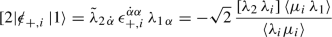
The polarisation vectors may be expressed as bi-spinors using the spinor-helicity variables associated with the momentum p ($p^{\alpha {\dot {\alpha }}}=\lambda ^{\alpha }\tilde \lambda ^{{\dot {\alpha }}}$) as

$$\displaystyle \begin{aligned} {} \epsilon_{+,i}^{\alpha{\dot{\alpha}}}= -\sqrt{2} \, \frac{\tilde\lambda^{{\dot{\alpha}}}_{i}\, \mu_{i}^{\alpha}}{\langle\lambda_{i}\mu_{i}\rangle}\, ,\qquad \epsilon_{-,i}^{\alpha{\dot{\alpha}}}= \sqrt{2} \, \frac{\tilde\mu^{{\dot{\alpha}}}_{i}\, \lambda_{i}^{\alpha}}{ [\tilde\lambda_{i}\tilde\mu_{i}]}\, . \end{aligned} $$

(1.124)

One directly checks the properties of Eq. (1.124) in this representation. We also find $h\, \epsilon _{\pm ,i}^{\alpha {\dot {\alpha }}}= \pm \epsilon _{\pm ,i}^{\alpha {\dot {\alpha }}}$, hence the helicity assignments check. The spinor pair $\mu _{i}$, $\tilde \mu _{i}$ appearing in the above are arbitrary reference spinors needed to define the polarisations. They parameterise a light-like reference momentum $r_{i}=\mu _{i}\tilde \mu _{i}$ associated to every leg $i=1,\ldots , n$ in a scattering amplitude. The only condition on the reference spinors is that they are nor parallel to $\lambda _{i}$ an $\tilde \lambda _{i}$:

$$\displaystyle \begin{aligned} \mu_{i}\neq c \lambda_{i}\, , \qquad \tilde\mu_{i}\neq c^{\ast} \tilde\lambda_{i}\, . \end{aligned} $$

(1.125)

Moreover, we see from Eq. (1.124) that $\epsilon _{\pm ,i} \cdot r_i = 0$.

Exercise 1.7 (Gluon Polarisations)

• (a) Show that the properties in Eq. (1.123), together with the gauge choice $\epsilon _{\pm ,i} \cdot r_i = 0$ (with $r_i^2=0$), lead to the representation of Eq. (1.124). Hint: expand the polarisation vector in a basis constructed from the spinors associated with $p_i^{\dot {\alpha }\alpha }$ and $r_i$.

• (b) Verify that the representation Eq. (1.124) fulfils the polarisation sum rule

  $$\displaystyle \begin{aligned} \sum_{h=\pm} \epsilon_{h,i}^{\mu} \epsilon_{h,i}^{*\nu} = - \eta^{\mu\nu} + \frac{p_i^{\mu} r_i^{\nu}+p_i^{\nu} r_i^{\mu}}{p_i \cdot r_i} \,. \end{aligned} $$

  (1.126)

For the solution see Chap. 5.

The appearance of the reference spinors $\mu _{i}$ and $\tilde \mu _{i}$ with associated reference momentum $r_{i}^{\alpha {\dot {\alpha }}} := \mu _{i}^{\alpha }\, \tilde \mu _{i}^{{\dot {\alpha }}}$ in the polarisation vectors corresponds to the freedom of performing local gauge transformations of the gauge field. To see this let us compute the infinitesimal change of the polarisation $\epsilon _{+}^{\alpha {\dot {\alpha }}}$ induced by an infinitesimal shift of the reference spinor $\mu \to \mu + \delta \mu$:

(1.127)

where we used Schouten’s identity (1.116) in step two. We see that the induced change of the polarisation vector $\epsilon _{+}^{\mu }$ is a gauge transformation $\delta \epsilon ^{\mu }= p^{\mu }\xi$. By transversality of the amplitude this implies the invariance under the shift $\mu \to \mu + \delta \mu$. Therefore the amplitude depends only on $\{\lambda _{i}, \tilde \lambda _{i}, h_{i}=\pm 1\}$, and we may freely choose the reference spinors $\mu _{i}$ and $\tilde \mu _{i}$ for every leg at our convenience—reflecting the local gauge invariance of the theory.

$\blacktriangleright$Spin$\mathbf {s=2}$

The polarisation of a graviton has the helicities $h=\pm 2$ and is captured by a symmetric rank-two tensor $\epsilon _{++/--}^{\mu \nu }(p)$. It is transverse

$$\displaystyle \begin{aligned} p_{\mu} \epsilon_{++/--}^{\mu\nu}(p) = 0 \,, \end{aligned} $$

(1.128)

and may be chosen to be traceless $\eta _{\mu \nu }\epsilon _{++/--}^{\mu \nu }(p)=0$. A very convenient parametrisation is given by doubling the gauge field polarisations:

$$\displaystyle \begin{aligned} {} \epsilon_{++}^{\mu\nu}(p)= \epsilon_{+}^{\mu}(p) \, \epsilon_{+}^{\nu}(p)\, , \qquad \epsilon_{--}^{\mu\nu}(p)= \epsilon_{-}^{\mu}(p) \, \epsilon_{-}^{\nu}(p)\, . \end{aligned} $$

(1.129)

In this way the above properties of transversality and tracelessness are consequences of the properties of the vector polarisations $\epsilon _{\pm }^{\mu }(p)$ in Eq. (1.123).

It is then straightforward to translate this into helicity spinor variables. We now have the spin-tensors

$$\displaystyle \begin{aligned} \epsilon_{++}^{\alpha\beta{\dot{\alpha}}{\dot{\beta}}} = \epsilon_{+}^{\alpha{\dot{\alpha}}}\, \epsilon_{+}^{\beta{\dot{\beta}}}\, , \qquad \quad \epsilon_{--}^{\alpha\beta{\dot{\alpha}}{\dot{\beta}}} = \epsilon_{-}^{\alpha{\dot{\alpha}}}\, \epsilon_{-}^{\beta{\dot{\beta}}}\, , \end{aligned} $$

(1.130)

using the polarisation bi-spinors of the gauge fields Eq. (1.124).

Again we have reference spinors $\mu _{i}$ and $\tilde \mu _{i}$ for each leg. The amplitude does not depend on this choice, and one may show that under a shift $\mu \to \mu + \delta \mu$ the graviton polarisation transforms as

$$\displaystyle \begin{aligned} \epsilon_{\mu\nu}\to \epsilon_{\mu\nu}^{\prime}=\epsilon_{\mu\nu} + 2 p_{(\mu}\xi_{\nu)} \,, \end{aligned} $$

(1.131)

by virtue of the same argument as in Eq. (1.127). This change of course leaves the amplitude invariant.

1.10 Colour Decompositions for Gluon Amplitudes

Let us now focus on non-Abelian gauge field theories and the management of colour. The tools to be developed will allow us to disentangle the colour degrees of freedom from the kinematic ones. There are two such formalisms for an efficient colour management which we shall discuss: the trace based, and the structure constant based formalism. Focussing on $\text{SU}(N_c)$ gauge theories coupled to matter, one mostly encounters two representations of the gauge group:

• Adjoint representation: gluons $A^a_\mu$ carry adjoint indices $a-1,\ldots ,N^2_c-1$;

• Fundamental & anti-fundamental representation: fermions and scalars carry fundamental indices $i=1,\ldots , N_c$ and $\bar i=1,\ldots , N_c$.

As discussed above, the generators of the $\text{SU}(N_c)$ algebra in the fundamental representation are $N_c\!\times \!N_c$ hermitian, traceless matrices $(T^a)_i{ }^{{j}}$ . We recall Eq. (1.48)

$$\displaystyle \begin{aligned} {} f^{abc}=-\frac{{\mathrm{i}}}{\sqrt{2}} \, {\mathrm{Tr}} \big(T^a [T^b, T^c] \big)\, , \end{aligned} $$

(1.132)

or $[T^a, T^b] {=} {\mathrm {i}}\sqrt {2} f^{abc} T^c$, with ${\mathrm {Tr}}(T^a T^b){=}\delta ^{ab}$. Moreover, we have the $\text{SU}(N_c)$ identity of Eq. (1.51),

$$\displaystyle \begin{aligned} {} (T^a)_{i_1}{}^{{j}_1}\, (T^a)_{i_2}{}^{{j}_2}= \delta_{i_1}{}^{{j}_2}\, \delta_{i_2}{}^{{j}_1} - \frac{1}{N_c}\delta_{i_1}{}^{{j}_1}\, \delta_{i_2}{}^{{j}_2} \, , \end{aligned} $$

(1.133)

which will be important for the trace based decomposition. It can be understood as a completeness relation for a basis of Hermitian matrices spanned by $\{{\mathbb{1} }, T^a\}$. Introducing a graphical representation for the structure constants and generators via

(1.134)

one may illustrate these two relations as in Fig. 1.1.

Fig. 1.1

Graphical representation of Eqs. (“reffasTr) and (“refSUNFierz) using (“refTagraphical) for the generators

Moreover, we recall the Jacobi identity for the structure constants of Eq. (1.50),

$$\displaystyle \begin{aligned} {} f^{abe} f^{ceg} + f^{bce} f^{aeg} + f^{cae} f^{beg} =0 \, , \end{aligned} $$

(1.135)

which we shall put to use in the structure constant based formalism.

1.10.1 Trace Basis

A look at the QCD Feynman rules of Sect. 1.4 tells us that the colour dependence of a given Feynman graph arises from its vertices. The three-gluon vertex in Eq. (1.65) carries one structure constant $f^{abc}$, whereas the four-gluon vertex in Eq. (1.66) contains two $f^{abc}$’s. Coupling to matter, the quark-anti-quark-gluon vertex Eq. (1.69) comes with a generator $(T^a)_i{ }^{ j}$. In order to work out the colour dependence of a given Feynman diagram in the trace basis, we replace all structure constants appearing in it by the trace formula (1.132). This transforms the expression to products of generators $(T^{a})_{i}{ }^{ j}$ with contracted and open indices. Open fundamental indices $(i, j)$ correspond to external quark lines in the diagram, open adjoint indices $(a)$ to the external gluon states. Contracted adjoint indices can be used to merge traces and products of generators by repeatedly applying the $\text{SU}(N_{c})$ identity (1.133):

$$\displaystyle \begin{aligned} {} (A\, T^{a} B)_{i}{}^{ j}\, (C\, T^{a} D)_{k}{}^{ l} = (A \, D)_{i}{}^{l}\, (C\, B)_{k}{}^{ j} -\frac{1}{N_{c}} (A\, B)_{i}{}^{j}\, (C\, D)_{k}{}^{ l} \, , \end{aligned} $$

(1.136)

where $A, B,C$ and D are arbitrary $N_{c}\times N_{c}$ matrices made of products of generators. By iterating this procedure we arrive at a final expression of traces and strings of generators $T^a$’s with only open adjoint and fundamental indices corresponding to the external states. They take the generic form

$$\displaystyle \begin{aligned} {\mathrm{Tr}}(T^{a_{1}}\cdots T^{a_{n}})\ldots {\mathrm{Tr}}(T^{b_{1}}\cdots T^{b_{m}})\, (T^{c_{1}} \cdots T^{c_{p}})_{i_{1}}{}^{ j_{1}} \ldots (T^{d_{1}} \cdots T^{d_{p}})_{i_{s}}{}^{j_{s}}\, . \end{aligned} $$

(1.137)

For pure gluon amplitudes there is a further simplification: in pure Yang-Mills theory the interaction vertices of the $\text{SU}(N_{c})$ and $\text{U}(N_{c})$ gauge groups are identical, as $f^{0bc}\!=\!0$ due to Eq. (1.132) where $T^{0}= {\mathbb{1} }/\sqrt {N_{c}}$ is the $\text{U}(1)$ generator. Hence, the ${1}/{N_{c}}$ part in the relation (1.136), responsible for tearing apart traces, is not active here. In conclusion, tree-level gluon amplitudes reduce to a single-trace structure, and can be brought into the colour-decomposed form

$$\displaystyle \begin{aligned} {} \mathcal{A}_{n}^{\text{tree}}(\{ a_{i}, h_{i},p_{i}\}) = \sum_{\sigma\in S_{n}/\mathbb{Z}_{n}}\, {\mathrm{Tr}}(T^{a_{\sigma_{1}}}\, T^{a_{\sigma_{2}}}\cdots T^{a_{\sigma_{n}}} )\, A_{n}^{\text{tree}}({\sigma_{1}}, {\sigma_{2}}, \ldots , \sigma_{n}) \, . \end{aligned} $$

(1.138)

Here $h_{i}$ denote the helicities and $a_{i}$ the adjoint colour indices of the external states, and we use the compact notation $\sigma = \{p_{\sigma },h_{\sigma }\}$ in the argument of the $A_{n}^{\text{tree}}$. The latter are called partial or colour-ordered amplitudes and carry all kinematic information. Moreover, $S_{n}/\mathbb {Z}_{n}$ is the set of all non-cyclic permutations of n elements, which is equivalent to $S_{n-1}$. Therefore for an n-particle amplitude we have $(n-1)!$ distinct colour-ordered amplitudes in the trace basis. For example in the four-point case we find

$$\displaystyle \begin{aligned} \begin{aligned} \mathcal{A}_{4}^{\text{tree}}& = {\mathrm{Tr}}(T^{a_{1}} T^{a_{2}} T^{a_{3}} T^{a_{4}} ) A_{4}^{\text{tree}}(1,2,3,4) + {\mathrm{Tr}}(T^{a_{1}} T^{a_{3}} T^{a_{4}} T^{a_{2}} )\, A_{4}^{\text{tree}}(1,3,4,2) \\ & \quad + {\mathrm{Tr}}(T^{a_{1}} T^{a_{4}} T^{a_{2}} T^{a_{3}} ) A_{4}^{\text{tree}}(1,4,2,3){+} {\mathrm{Tr}}(T^{a_{1}} T^{a_{2}} T^{a_{4}} T^{a_{3}} ) A_{4}^{\text{tree}}(1,2,4,3) \\ & \quad + {\mathrm{Tr}}(T^{a_{1}} T^{a_{4}} T^{a_{3}} T^{a_{2}} ) A_{4}^{\text{tree}}(1,4,3,2) {+} {\mathrm{Tr}}(T^{a_{1}} T^{a_{3}} T^{a_{2}} T^{a_{4}} ) A_{4}^{\text{tree}}(1,3,2,4) . \end{aligned} \end{aligned} $$

(1.139)

This is the promised separation of colour and kinematical degrees of freedom. The colour ordered amplitudes $A_{n}$ are simpler than the full amplitudes $\mathcal {A}_{n}$, as they are individually gauge invariant. This is due to the fact that any shift of a polarisation $\epsilon _{i}\to p_{i}$ in (1.138) will lead to a vanishing left-hand side for $\mathcal {A}_{n}$. On the right-hand side the colour factors form a linearly independent basis, hence the individual factors of $A_{n}$ need to vanish individually. In addition, they exhibit poles only whenever cyclically adjacent momenta go on-shell, $(p_{i}+p_{i+1}+\cdots + p_{i+s})^{2}\to 0$, see Fig. 1.2. This property will be exploited in Chap. 2.

Fig. 1.2

Some of the possible poles in a colour-ordered Feynman diagram

For tree-level gluon-quark-anti-quark amplitudes with a single quark line one has

$$\displaystyle \begin{aligned} \begin{aligned} \mathcal{A}_{n,q\bar q}^{\text{tree}} \Big(\{ a_{i}, h_{i},p_{i}\}|\Big\{i,q_{1}^{h_{q_{1}}}, j,\bar{q}_{2}^{h_{q_{2}}}\Big\}\Big) & = \sum_{\sigma\in S_{n-2}} (T^{a_{\sigma_{1}}}\, \cdots T^{a_{\sigma_{n-2}}})_{i}{}^{j}\, \\ & \times A_{n,q\bar q}^{\text{tree}}\Big(\sigma_{1}, \ldots, {\sigma_{n-2}}| q_{1}^{h_{q_{1}}} , \bar{q}_{2}^{h_{q_{2}}}\Big) \, . \end{aligned} \end{aligned} $$

(1.140)

Increasing the number of quark lines to $m>1$ yields a more involved structure, as more strings and factors of $1/N_c$ appear. Here the m quark lines will yield m products of strings in T-matrices, $(T^{a_1}\, T^{a_2} \cdots T^{a_r})_{i_s}{ }^{{j}_s}$, where the adjoint indices are either contracted with an outer gluon leg or connect to another quark line. Using the $\text{SU}(N_{c})$ identity (1.136) for these internal contractions leads to a final basis of m products of open T-matrix strings with only external adjoint indices. The general construction of this colour-decomposition is rather involved and we shall not discuss it here. We refer to [11,12,13,14] for a detailed analysis. In this case, some of the colour factors also include explicit factors of $1/N_c$ stemming from the last term in Eq. (1.136). Nevertheless, all of the kinematical dependencies can still be constructed from suitable linear combinations of the partial amplitudes for external quarks, anti-quarks and external gluons generated by the colour-ordered Feynman diagrams. Hence, the partial amplitudes are the atoms of gauge-theory scattering amplitudes.

At loop level, pure gluon amplitudes contain also multi-trace contributions arising from the merging performed using Eq. (1.133). For example, at one loop one has

$$\displaystyle \begin{aligned} \begin{aligned} {} \mathcal{A}_{n}^{\text{1-loop}}(\{ a_{i}, h_{i},p_{i}\}) &= N_c\, \sum_{\sigma\in S_{n}/\mathbb{Z}_{n}}\, {\mathrm{Tr}}(T^{a_{\sigma_{1}}}\, T^{a_{\sigma_{2}}}\cdots T^{a_{\sigma_{n}}} )\, A_{n;1}^{(1)}(\sigma_{1}, \ldots , \sigma_{n} ) \\ + \sum_{i=2}^{[n/2]+1}\, \sum_{\sigma\in S_n/\mathbb{Z}_n} & {\mathrm{Tr}}(T^{a_{\sigma_{1}}} \cdots T^{a_{\sigma_{i-1}}} )\, {\mathrm{Tr}}(T^{a_{\sigma_{i}}}\cdots T^{a_{\sigma_{n}}})\, A_{n;i}^{(1)}(\sigma_{1}, \ldots , \sigma_{n} )\, , \end{aligned} \end{aligned} $$

(1.141)

where the $A_{n;1}^{(1)}$ are called the primitive (colour-ordered) amplitudes, and the $A_{n;c>1}^{(1)}$ are the higher primitive amplitudes, $[n]$ is the lower integer part of n. The latter can be expressed as linear combinations of the primitive ones [15]. In the large-$N_{c}$ limit the single-trace contributions are enhanced: one speaks of the leading-colour contributions. In colour-summed cross sections, which are of interest for computing collider physics observables, the contribution of the higher primitive amplitudes is suppressed by a factor of $1/N_{c}^2$.

1.10.2 Structure Constant Basis

An alternative basis for the colour decomposition of pure-gluon amplitudes employs the structure constants $f^{abc}$ and is due to Del Duca, Dixon and Maltoni (DDM) [16]. To begin with, we consider the colour dependence of an n-gluon tree amplitude. This may be represented as a sum over only tri-valent graphs with vertices linear in $f^{abc}$. In order to reach this tri-valent representation we artificially “blow” up a four-valent gluon vertex to sums of products of tri-valent vertices. This is done by multiplying it by $1=q^{2}/q^{2}$ where ${\mathrm {i}}/q^{2}$ is the “blown up” propagator. Concretely, if we go back to the Feynman rule of Eq. (1.66) for the four-gluon vertex, we rewrite

$$\displaystyle \begin{aligned} f^{abe}f^{cde} = f^{abe}\, \frac{\delta_{ef} (p_{a}+p_{b})^{2}}{(p_{a}+p_{b})^{2}}f^{cdf} \,, \end{aligned} $$

(1.142)

where $p_{a}$($p_{b}$) is the momentum flowing into leg a (b), and analogously for the other two ff-terms. The resulting structure will then be a trivalent tree as in Fig. 1.3.

Fig. 1.3

Typical colour tree in a structure constant based expansion

Now we use the Jacobi identity (1.50) for the structure constants,

(1.143)

in order to successively shrink branched trees to branchless ones, resulting in a final “half-ladder” expression. The shrinking of a branched tree is thereby performed via the operation

(1.144)

In summary, one may colour-reduce any diagram, e.g. as depicted in Fig. 1.3, to the “half-ladder” structure shown in Fig. 1.4. In this way we can completely reduce an amplitude to a sum of colour-ordered amplitudes in the half-ladder basis in colour space:

$$\displaystyle \begin{aligned} {} \begin{aligned} \mathcal{A}_{n}^{\text{tree}}(\{ a_{i}, h_{i},p_{i}\}) \!=\! \\ \sum_{\sigma\in S_{n-2}}\, f^{a_{1}a_{\sigma_{2}}e_{1}} & \, f^{e_{1}a_{\sigma_{3}}e_{2}} \, f^{e_{2}a_{\sigma_{4}}e_{3}} \cdots f^{e_{n-3}a_{\sigma_{n-1}}a_{n}} A_{n}^{\text{tree}}(1, {\sigma_{2}}, \ldots , {\sigma_{n-1}}, n) \, , \end{aligned} \end{aligned} $$

(1.145)

where we now sum over the permutations $\sigma$ of the $n{-}2$ elements $\{2,3,\ldots , n-1\}$. The half-ladder colour basis fixes two (arbitrary) legs, here 1 and n, see Fig. 1.4.

Fig. 1.4

Half-ladder form

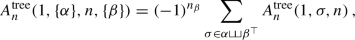
In consequence, the DDM basis consists of $(n-2)!$ independent partial amplitudes. This is to be contrasted with the $(n-1)!$ partial amplitudes that we found in the trace basis. Hence, there must exist non-trivial identities between colour-ordered amplitudes allowing one to reduce the basis accordingly. These are known as Kleiss-Kuijf relations [17], and take the form

(1.146)

where $n_{\beta }$ denotes the number of elements in the set $\beta$, and $\beta ^{\top }$ is the set $\beta$ with reversed ordering. The shuffle or ordered permutation ${\displaystyle \alpha {\sqcup \!\sqcup } \beta ^{\top }}$ of the two sets merges $\alpha$ and $\beta ^{\top }$ while preserving the individual orderings of $\alpha$ and $\beta ^{\top }$. An example illustrates this:

$$\displaystyle \begin{aligned} \{12\} {\sqcup\!\sqcup} \{34\}^{\top}= \{1243\}+\{1423\}+\{1432\}+\{4123\}+\{4312\}+\{4132\} \,. \end{aligned}$$

In fact, one can prove the Kleiss-Kuijf relations (1.146) by rewriting the DDM basis in terms of the trace basis discussed above.

It turns out that there exists a further non-trivial identity between colour-ordered amplitudes, allowing one to further reduce the basis of colour-ordered (or partial) amplitudes to $(n-3)!$ independent elements. This is due to the Bern-Carrasco-Johansson relation [18, 19], to be discussed in Chap. 2.7. It takes the schematic form

$$\displaystyle \begin{aligned} {} A_{n}^{\text{tree}}(\sigma_{1},\ldots,\sigma_{n}) = \sum_{\rho\in S_{n-3}} K^{(\sigma)}_{\rho} A_{n}^{\text{tree}}(1,2,{\rho_{3}},\ldots, \rho_{n-1},n)\, , \end{aligned} $$

(1.147)

with coefficients $K^{(\sigma )}_{\rho }$ depending on the external momenta. Finally, we note that there is also a useful generalisation of the DDM basis to include fundamental matter that we will not discuss here, see [20, 21].

Colour-Ordered Feynman Rules One may write down colour-ordered Feynman rules that generate the colour-ordered (partial) amplitudes upon stripping off the colour factors from the usual Feynman rules. This is trivial for the gluon and quark propagators (working in Feynman gauge):

(1.148)

To obtain the colour-ordered vertex rules one inserts into the standard Feynman rules of Sects. 1.4 and 1.5 the trace expression (1.132) for $f^{abc}$, and together with the identity (1.133) reduces everything to a string of generators. Extracting only a single ordering of the $T^{a}$’s then yields the colour-ordered vertices:

(1.149)

Similarly, in the scalar QCD sector we have the propagator

(1.150)

and the vertices

(1.151)

Exercise 1.8 (Colour-Ordered Feynman Rules)

Derive the form of the colour-ordered four-gluon vertex in Eq. 1.149 from the Feynman rules of Eq. (1.66). For the solution see Chap. 5.

$\blacktriangleright$General Properties of Colour-Ordered Amplitudes

Due to the factorisation of the colour degrees of freedom, the partial or colour-ordered amplitudes are individually gauge invariant. Next to the Kleiss-Kruif (1.146) and Bern-Carrasco-Johansson (1.147) relations, they obey further general properties which reduce considerably the number of independent structures. We list them below, denoting by $A(1,2,\ldots ,n)$ the colour-ordered amplitudes, where the argument i refers to a colour-ordered gluon, while a quark (anti-quark) leg is denoted by $i_{q}$ ($i_{\bar {q}}$).

• 1. Cyclicity:

  $$\displaystyle \begin{aligned} A(1,2,\ldots, n) = A(2,\ldots, n,1) \, , \end{aligned} $$

  (1.152)

  which follows from the cyclicity of the trace and the definition of Eq. (1.138).

• 2. Parity:

  $$\displaystyle \begin{aligned} A(\bar 1, \bar 2,\ldots,\bar n)= A(1,2,\ldots, n) \Big|{}_{\langle ij\rangle\to [ji], [ij] \to\langle ji\rangle }\, . \end{aligned} $$

  (1.153)

  Here the bar over the particle number denotes the inversion of the particle’s helicity. Note the flip in the helicity spinor brackets under parity.

• 3. Charge conjugation:

  $$\displaystyle \begin{aligned} A(1_q,2_{\bar q},3,\ldots, n) = - A(1_{\bar q},2_{q},3,\ldots, n)\ , \end{aligned} $$

  (1.154)

  that is, flipping the helicity of a quark line changes the sign of the amplitude. This descends from the colour-ordered gluon-quark-anti-quark vertex above.

• 4. Reflection:

  $$\displaystyle \begin{aligned} A(1,2,\ldots, n) = (-1)^n\, A(n,n-1,\ldots,1)\, . \end{aligned} $$

  (1.155)

  This relation follows from the anti-symmetry of the colour-ordered gluon vertices under reflection of all legs. It also holds in the presence of quark lines but only at tree level.

• 5. Photon or $\text{U}(1)$ decoupling identity:

  $$\displaystyle \begin{aligned} {} \sum_{\sigma\in \mathbb{Z}_{n-1}} A(\sigma_1, \ldots , \sigma_{n-1}, n) =0\, , \end{aligned} $$

  (1.156)

  where $\sigma = \{\sigma _1, \ldots , \sigma _{n-1}\}$ are cyclic permutations of $\{1, 2, \ldots , n-1\}$. This powerful identity follows from Eq. (1.138) and the fact that a gluon amplitude with a single photon vanishes since $f^{0bc}{=}0$. Here 0 is the colour index of the $\text{U}(1)$ generator $T^{0}={\mathbb{1} }/\sqrt {N_c}$.

• 6. We restate the Kleiss-Kuijf relations [17] of Eq. (1.146),

  

  (1.157)

  which may be derived by the transition from the DDM basis to the trace basis.

• 7. Finally, there is a final set of relations emerging from the double copy or Bern-Carrasco-Johansson [18] duality between graviton and gluon amplitudes:

  $$\displaystyle \begin{aligned} {} \sum_{i=2}^{n-1}p_{1}\cdot (p_{2} + \ldots + p_{i})\, A^{\text{tree}}_{n}(2,\ldots, i,1, i+1,\ldots,n) =0 \, . \end{aligned} $$

  (1.158)

  This we will discuss in the later Sect. 2.7 but quote already for completeness.

In summary there are $(n-1)!$ independent colour-ordered gluon amplitudes of multiplicity n.

Exercise 1.9 (Independent Gluon Partial Amplitudes)

Use the above relations amongst the colour-ordered amplitudes to determine the independent set of colour-ordered amplitudes for four- and five-gluon scattering. For the solution see Chap. 5.

1.11 Colour-Ordered Amplitudes

Let us now begin with the actual evaluation of the first pure gluon tree-amplitudes using the colour-ordered Feynman rules and the spinor-helicity formalism. In fact, we will see that large classes of gluon helicity amplitudes vanish!

1.11.1 Vanishing Tree Amplitudes

Let us restrict to tree-level amplitudes with multiplicities $n>3$ here, as there are subtleties for the three-point gluon amplitudes to be discussed later. Our freedom to choose an arbitrary light-like reference momentum $r_{i}^{{\dot {\alpha }}\alpha }=\mu _{i}^{\alpha }\, \tilde \mu _{i}^{{\dot {\alpha }}}$ in the definition of the gluon polarisation vectors $\epsilon _{\pm , i}$ in Eq. (1.124) for every leg may be used to show that entire classes of helicity gluon amplitudes vanish.

Using Eq. (1.124) we find the polarisation vector products of legs i and j to be

(1.159)

with the only restriction on the reference spinors of leg i being distinct to the outflowing momentum of that leg, i.e. $\mu _{i}\neq \lambda _{i}$ and $\tilde \mu _{i}\neq \tilde \lambda _{i}$. Clearly, if we choose the reference spinors of legs i and j to be identical, we have that

$$\displaystyle \begin{aligned} \epsilon_{+, i}\cdot \epsilon_{+, j}= 0 =\epsilon_{-, i}\cdot \epsilon_{-, j}\qquad \forall\, i,j\, , {} \end{aligned} $$

(1.160)

due to $\langle \mu _{i}\mu _{j}\rangle =0= [\mu _{i}\mu _{j}]$ for that choice. Let us see how to use this in order to identify vanishing trees.

An n-gluon tree amplitude must depend on the n-polarisation vectors involved, which have to be contracted either with themselves (as $\epsilon _{i}\cdot \epsilon _{j}$) or with the external momenta (as $p_{i}\cdot \epsilon _{j}$). Now, what is the minimal number of polarisation vector contractions $\epsilon _{i}\cdot \epsilon _{j}$ arising in the terms that constitute an n-gluon tree-amplitude? To find this number, we need to look at graphs which maximise the number of momentum-polarisation contractions, i.e. $p_{i}\cdot \epsilon _{j}$. This implies looking at graphs built entirely out of three-point vertices. Pure three-point vertex n-gluon trees are made of $(n-2)$-vertices. This follows immediately from the half-ladder form in the DDM basis, cf. Fig. 1.4.

As an n-leg graph contains n distinct polarisation vectors, we conclude that any n-gluon amplitude will consist of terms containing $at\,\, least$ one polarisation contraction $\epsilon _{i}\cdot \epsilon _{j}$ (as this maximum configuration is attained by purely trivalent trees). Armed with this insight, we now prove the vanishing of three classes of tree-amplitudes.

• 1. Choosing the reference momenta $r_{i}$ of an n-gluon tree-amplitude uniformly as in Eq. (1.160) implies that

  $$\displaystyle \begin{aligned} A^{\text{tree}}_{n}(1^{+},2^{+},\ldots, n^{+})=0\, , {} \end{aligned} $$

  (1.161)

  as at least one $\epsilon _{+, i}\cdot \epsilon _{+, j}$ contraction must arise.

• 2. Similarly, the gluon tree-amplitude with one flipped helicity state vanishes:

  $$\displaystyle \begin{aligned} A^{\text{tree}}_{n}(1^{-},2^{+},\ldots, n^{+})=0\, . {} \end{aligned} $$

  (1.162)

  This follows from the reference momenta choice

  $$\displaystyle \begin{aligned} r_{1}=r\neq p_{1}\, \qquad \text{and} \qquad r_{2}=\ldots= r_{n}=p_{1}\, , \end{aligned} $$

  (1.163)

  as then all terms containing a $\epsilon _{+, i}\cdot \epsilon _{+, j}=0$ contraction with $i,j\in \{2,\ldots ,n\}$ vanish, and $\epsilon _{+, i}\cdot \epsilon _{-, 1}=0$ due to Eq. (1.159) by the specific choice above.

• 3. Finally, the $q\bar q g^{n-2}$ amplitudes vanish if all gluons have identical helicity:

  $$\displaystyle \begin{aligned} A^{\text{tree}}_{n}(1^{-}_{\bar q},2^{+}_{q},3^{+}\ldots, n^{+})=0\, . {} \end{aligned} $$

  (1.164)

  Due to the presence of a quark line there is at least one contraction of the form

  

  (1.165)

  in every term constituting the amplitude. Choosing the gluon-polarisation reference momenta uniformly as $r_{i}=\mu _{i}\, \tilde \mu _{i} = \lambda _{1}\, \tilde \lambda _{1}$ for all $i\in \{3,\ldots , n\}$ yields , and hence the vanishing of Eq. (1.164).

By parity the vanishing of Eqs. (1.161) and (1.162) implies

$$\displaystyle \begin{aligned} A^{\text{tree}}_{n}(1^{\pm},2^{-},\ldots, n^{-})=0\, . {} \end{aligned} $$

(1.166)

Hence the first non-trivial class of pure gluon tree-amplitudes is the one with two flipped helicities, $A^{\text{tree}}_{n}(1^{-},2^{+},\ldots , (i-1)^{+},i^{-},(i+1)^{+},\ldots , n^{+})$, known as maximally helicity violating (MHV) amplitudes.

To understand this name recall that in our convention all momenta are out-going. The MHV amplitudes describes, for example, a process in which all incoming gluons have one helicity and all but two outgoing gluons—the maximal allowed number—have the opposite helicity: flipping the momentum entails a flip in helicities. Hence, helicity is not conserved and this process is maximally helicity violating.

Similarly, we have for the single-quark-line-gluon amplitude that

$$\displaystyle \begin{aligned} A^{\text{tree}}_{n}(1^{-}_{\bar q},2^{+}_{q},3^{-}\ldots, n^{-})=0\, , {} \end{aligned} $$

(1.167)

by choosing $q_{i}=\mu _{i}\, \tilde \mu _{i} = \lambda _{2}\, \tilde \lambda _{2}$ for all $i\in \{3,\ldots , n\}$. Alternatively, this may be seen by a parity and charge conjugation transformation of Eq. (1.164).

As a matter of fact, the vanishing of these mostly-plus (or minus) amplitudes can be understood from a hidden supersymmetry in tree-level quark-gluon tree-amplitudes, see [22, 23] for a discussion.

Amplitudes comprised of 3 positive helicity and $(n-3)$ negative helicity gluons are known as next-to maximally helicity violating (NMHV) amplitudes and so on, see Fig. 1.5

Fig. 1.5

The MHV classification of gluon amplitudes: $A_{n,m}$ denotes an n-gluon amplitude with m positive helicity states. Parity acts as a mirror across the vertical axis as $A_{n,m} \leftrightarrow A_{n,n-m}$. For example the NMHV $A_{5,3}$ amplitude may be obtained from the parity mirror of the MHV $A_{5,2}$ one. Hence, the lowest multiplicity non-trivial NMHV amplitude is the $A_{6,3}$

1.11.2 The Three-Gluon Tree-Amplitudes

We now want to establish the smallest amplitudes in gluon scattering. As a matter of fact, three-point amplitudes of massless particles are very special objects. Due to kinematics all Mandelstam invariants vanish, $p_{i}\cdot p_{j}=0$ for all $i,j$. This follows from momentum conservation

$$\displaystyle \begin{aligned} p_{1}^{\mu}+p_{2}^{\mu}+p_{3}^{\mu}=0 \,, \end{aligned} $$

(1.168)

which, with $p_i^2=0$ for all i, implies that

$$\displaystyle \begin{aligned} p_{i}\cdot p_{j}=0 \quad \forall \, i,j\in \{1,2,3\} \, . \end{aligned} $$

(1.169)

Hence for real momenta this implies the vanishing of the spinor brackets $\langle ij\rangle$ and $[ij]$, which are the building blocks of the amplitudes for massless particles. There is thus no Lorentz invariant object one could write down, and therefore the three-particle amplitude must vanish. The situation is different if one allows for complex momenta$p_{i} \in {\mathbb {C}^{4}}$. In this case the helicity spinors $\lambda _{i}$ and $\tilde {\lambda }_{i}$ are independent, and the conditions $p_{i} \cdot p_{j} =0$ can be solved either by $[i j] = 0$or by $\langle i j\rangle =0$. Hence either $\tilde \lambda _{1}^{\alpha } \propto \tilde \lambda _{2}^{\alpha } \propto \tilde \lambda _{3}^{\alpha }$ (collinear right-handed spinors) or $\lambda _{1}^{\alpha } \propto \lambda _{2}^{\alpha } \propto \lambda _{3}^{\alpha }$ (collinear left-handed spinors) solve the constraints $p_{i}\cdot p_{j}=0$. The two choices correspond to the three-gluon MHV${ }_{3}$ amplitude

$$\displaystyle \begin{aligned} \begin{array}{rcl} {} A_{3}^{\text{tree}}(1^{-},2^{-},3^{+}) = {\mathrm{i}} g\frac{ \langle12\rangle^3 }{\langle23\rangle\langle31\rangle}\,,\qquad \lbrack 12\rbrack=\lbrack2 3\rbrack = \lbrack 3 1\rbrack = 0\,, \end{array} \end{aligned} $$

(1.170)

and the dual $\overline {\text{MHV}}_{3}$ amplitude

$$\displaystyle \begin{aligned} \begin{array}{rcl} {} A_{3}^{\text{tree}}(1^{+},2^{+},3^{-}) = - {\mathrm{i}} g\frac{ [12]^3 }{ [23] [31]}\,,\qquad \langle1 2\rangle= \langle2 3\rangle = \langle3 1\rangle = 0\,, \end{array} \end{aligned} $$

(1.171)

respectively. The two are related by a parity transformation, which flips the helicity weights and exchanges $\langle i j \rangle \leftrightarrow [ji]$.

As a useful exercise in spinor gymnastics, we will now derive these amplitudes from the colour-ordered Feynman rules. Using the three-gluon vertex in Eq. (1.149) we find

(1.172)

where the polarisation vector contractions are given in Eq. (1.159). Choosing the same reference-momentum spinor $\mu _{1}=\mu _{2}=\mu _{3}=\mu$ for the gluons we have $\epsilon _{-,1} {\cdot } \epsilon _{-,2} =0$. Then, by using momentum conservation and transversality $p_i\cdot \epsilon _i=0$, we arrive at

(1.173)

From Eq. (1.159) we derive the following expressions,

$$\displaystyle \begin{aligned} \begin{aligned} \epsilon_{-,2}\!\cdot\!\epsilon_{+,3}&= -\frac{\langle 2 \mu\rangle[3\mu ] }{[ 2 \mu] \langle 3 \mu\rangle} \, , \qquad \qquad \, \epsilon_{-,1}\!\cdot\!\epsilon_{+,3}= -\frac{\langle 1 \mu\rangle[3\mu ] }{[ 1 \mu] \langle 3 \mu\rangle} \, , \\ p_2\cdot \epsilon_{-,1}&= \frac{1}{\sqrt{2}}\frac{\langle 12 \rangle[2 \mu]}{[1 \mu]}\, , \qquad \quad \ \ \, p_1\cdot \epsilon_{-,2}= -\frac{1}{\sqrt{2}}\frac{\langle 12 \rangle[1 \mu]}{[2 \mu]}\, , \end{aligned} \end{aligned} $$

(1.174)

and therefore

(1.175)

Finally, we use three-point momentum conservation to simplify

$$\displaystyle \begin{aligned} \frac{[3\mu] }{[1\mu]}=\frac{\langle 23\rangle [3\mu] }{\langle 23\rangle[1\mu]}=\frac{\langle12\rangle}{\langle23\rangle}\, , \qquad \quad \frac{[3\mu] }{[2\mu]}=\frac{\langle 13\rangle [3\mu] }{\langle 13\rangle[2\mu]}=\frac{\langle12\rangle}{\langle31\rangle}\, , \end{aligned} $$

(1.176)

thus arriving at the result in Eq. (1.170). One could repeat this calculation for the scattering of three gravitons, this time using the three-graviton vertex of Eq. (1.87), arriving at a result proportional to $\big [ A_{3}^{\text{tree}}(1^{-}, 2^{-}, 3^{+})\big ]^2$. The involved expression for the vertex Eq. (1.87) gives no hints of such a remarkable squaring relation! We shall take up this discussion in Chap. 2 again.

1.11.3 Helicity Weight

There is an important consistency requirement for scattering amplitudes based on checking their correct helicity weights. This is encoded in the following relation [24]:

$$\displaystyle \begin{aligned} {} \hat h_{i}\, A= -\frac{1}{2} \left( \lambda_i^\alpha \ \frac{\partial}{\partial \lambda_i^\alpha} - \tilde{\lambda}_i^{\dot{\alpha}}\frac{\partial}{\partial \tilde{\lambda}_i^{\dot{\alpha}}}\right) \, A \, = \, h_i \, A\, , \end{aligned} $$

(1.177)

where $h_i$ is the helicity of particle i. When combined with Lorentz invariance, this relation can be used to determine the functional form of the three-point amplitudes of particles of any spin. As we argued, above a massless three-particle amplitude in complexified momentum space can either only depend on $\langle i\, j\rangle$ with $[ i\, j] {=}0$ for all particles or vice versa. If we choose the MHV situation $[ i\, j] {=}0$ for the helicity assignment $1^{-s}, 2^{-s}, 3^{+s}$, one can immediately see, using (1.177), that the answer must have the form

$$\displaystyle \begin{aligned} {} A(1^{-s}, 2^{-s}, 3^{+s}) \sim \big[ A(1^{-}, 2^{-}, 3^{+})\big]^s\, . \end{aligned} $$

(1.178)

In fact, for the gluon-amplitude with $s{=}1$, the conditions

$$\displaystyle \begin{aligned} \hat h_{1} A_{3}^{\text{MHV}}= - A_{3}^{\text{MHV}}\, , \quad \hat h_{2} A_{3}^{\text{MHV}}= - A_{3}^{\text{MHV}}\, , \quad \hat h_{3} A_{3}^{\text{MHV}}= + A_{3}^{\text{MHV}}\, \quad \end{aligned} $$

(1.179)

uniquely fix the amplitude to take the form $A(1^-, 2^-, 3^+) \!\sim \!{\langle 1\, 2\rangle ^3}/ ({\langle 2\, 3\rangle \langle 3\, 1\rangle })$. This may be seen as an independent derivation of both the 3-point gluon and graviton amplitudes—without referring to any Lagrangian!

Exercise 1.10 (The $\overline {\text{MHV}}_{3}$ Amplitude)

Derive the anti-MHV three-gluon amplitude (1.171) using the colour-ordered Feynman rules. For the solution see Chap. 5.

Example: A Four-Gluon Tree-Amplitude

We shall now compute the simplest non-trivial tree-level colour-ordered gluon amplitude, namely the four-gluon MHV-amplitude with a split helicity distribution $A_{4}^{\text{tree}}(1^{-},2^{-},3^{+},4^{+})$. Employing the colour-ordered Feynman rules of Eq. (1.149) we see that the three diagrams of Fig. 1.6 contribute to the amplitude.

Fig. 1.6

The three colour-ordered graphs contributing to the four-gluon split helicity MHV amplitude

Its computation is again considerably simplified by a clever choice of the reference momenta $r_i=\mu _{i}\, \tilde \mu _{i}$ of the gluon polarisations,

$$\displaystyle \begin{aligned} r_{1}=r_{2}=p_{4}\, , \qquad r_{3}=r_{4}=p_{1} \, , {} \end{aligned} $$

(1.180)

where $p_{i}$ denote the physical external momenta. Then one sees, using Eq. (1.159), that the polarisation-vector products

$$\displaystyle \begin{aligned} \epsilon_{-, 1}\cdot\epsilon_{-, 2} = \epsilon_{+, 3}\cdot\epsilon_{+, 4} = \epsilon_{-, 1}\cdot\epsilon_{+, 4} = \epsilon_{-, 2}\cdot\epsilon_{+, 4} = \epsilon_{-, 1}\cdot\epsilon_{+, 3} = 0 {} \end{aligned} $$

(1.181)

all vanish, and that the only non-vanishing contraction is

$$\displaystyle \begin{aligned} {} \epsilon_{-, 2}\cdot\epsilon_{+, 3} = - \frac{\langle\mu_{3}\,\lambda_{2}\rangle \, [\mu_{2}\, \lambda_{3}]} {\langle\lambda_{3}\, \mu_{3}\rangle\, [\lambda_{2}\, \mu_{2}]} = - \frac{\langle12\rangle\, [34]}{\langle13\rangle\, [24]}\, . \end{aligned} $$

(1.182)

Of course it is mandatory to use the same choice of reference momenta for all graphs.

Diagram I

$$\displaystyle \begin{aligned} \begin{aligned} (\text{I}) = \left(\frac{{\mathrm{i}} g}{\sqrt{2}}\right )^{2}\, \frac{-{\mathrm{i}}\,\eta_{\mu\nu}}{s_{12}}\, & \Big [ \epsilon_{-,2}^{\mu} \, (p_{2q}\cdot \epsilon_{-,1}) + \epsilon_{-,1}^{\mu} \, (p_{q1}\cdot \epsilon_{-,2})\, \Big ] \\ \times \Big [ \epsilon_{+,4}^{\nu} \, & (p_{4(-q)}\cdot \epsilon_{+,3}) + \epsilon_{+,3}^{\nu} \, (p_{(-q)3}\cdot \epsilon_{+,4})\, \Big ] \, , \end{aligned} \end{aligned} $$

(1.183)

with $q=-p_{1}-p_{2}=p_{3}+p_{4}$, $s_{12}=(p_{1}+p_{2})^{2}=\langle 12\rangle [21]$ and $p_{ij}=p_{i}-p_{j}$. Due to only $\epsilon _{-,2}\cdot \epsilon _{+,3}$ surviving in the contraction, we have

$$\displaystyle \begin{aligned} \begin{aligned} (\text{I}) & = \frac{{\mathrm{i}} g^{2}}{2s_{12}}\, (\epsilon_{-,2}\cdot\epsilon_{+,3})\, (p_{2}+p_{1}+p_{2})\cdot\epsilon_{-,1}\, (-p_{3}-p_{4}-p_{3})\cdot\epsilon_{+,4} \\ & = -\frac{2{\mathrm{i}} g^{2}}{s_{12}}\,(\epsilon_{-, 2}\cdot\epsilon_{+, 3})\,(p_{2}\cdot\epsilon_{-, 1})\, (p_{3}\cdot\epsilon_{+, 4}) \\ & = - \frac{2{\mathrm{i}} g^{2}}{s_{12}}\, \left ( - \frac{\langle12\rangle\, [34]}{\langle13\rangle\, [24]}\, \right )\, \left ( \frac{1}{\sqrt{2}}\, \frac{\langle12\rangle\, [24]}{ [14]}\, \right )\, \left ( \frac{1}{\sqrt{2}}\, \frac{\langle13\rangle\, [34]}{\langle14\rangle}\, \right ) \\ & = {\mathrm{i}} g^{2}\, \frac{\langle12\rangle\, [34]^{2}}{ [12]\, \langle14\rangle\, [41]}\, , \end{aligned} \end{aligned} $$

(1.184)

where in the second line we used $\displaystyle p_{2}\cdot \epsilon _{-,1}= {\textstyle \frac {1}{\sqrt {2}}}\, {\textstyle \frac {\langle 12\rangle \, [2\,\mu _{1}]}{ [1\mu _{1}]}} \stackrel {\mu _{1}=4}{=} {\textstyle \frac {1}{\sqrt {2}}}\, {\textstyle \frac {\langle 12\rangle \, [24]}{ [14]}}$, and similarly for $p_{3}\cdot \epsilon _{+,4}$. The last expression can be rewritten exclusively in terms of $\lambda _{i}$ spinors as

(1.185)

Here in the first step the four-point kinematical relation $s_{12}=\langle 12\rangle \, [21]=s_{34}=\langle 34\rangle \, [43]$ was used.

Diagram II

Using again the fact that the only non-vanishing contraction is that of Eq. (1.182) we find a vanishing result:

$$\displaystyle \begin{aligned} \hspace{-9pt}(\text{II}) & \propto \frac{-{\mathrm{i}}}{2s_{14}}\, (\epsilon_{2}\cdot\epsilon_{3})\, \Big [\, (p_{23}\cdot\epsilon_{1})\, (p_{1(-q)}\cdot\epsilon_{4}) + (p_{23}\cdot\epsilon_{4})\, (p_{(-q)4}\cdot\epsilon_{1}) \, \Big ] =0\, . \end{aligned} $$

(1.186)

Here with $q=p_{1}+p_{4}$ we have $p_{1(-q)}\cdot \epsilon _{4}=2\, p_{1}\cdot \epsilon _{4}=0$, which vanishes by virtue of our choice $q_{4}=p_{1}$ of Eq. (1.180). Similarly, $p_{(-q)4}\cdot \epsilon =-2\, p_{4}\cdot \epsilon _1 =0$ as $q_{1}=p_{4}$. Hence diagram II gives no contribution.

Diagram III

The same holds true for the third graph as

$$\displaystyle \begin{aligned} (\text{III})\propto 2\, (\epsilon_{2}\cdot\epsilon_{4})\, (\epsilon_{1}\cdot\epsilon_{3}) - (\epsilon_{2}\cdot\epsilon_{3})\, (\epsilon_{1}\cdot\epsilon_{4})- (\epsilon_{2}\cdot\epsilon_{1})\, (\epsilon_{3}\cdot\epsilon_{4}) = 0 \, , \end{aligned} $$

(1.187)

where at least one of the vanishing contractions in Eq. (1.181) appears in each term.

In summary, we have established the following compact result for the split-helicity MHV four-point amplitude:

$$\displaystyle \begin{aligned} A_{4}^{\text{tree}}(1^{-},2^{-},3^{+},4^{+}) = {\mathrm{i}} g^{2}\frac{\langle12\rangle^{4}}{\langle12\rangle\,\langle23\rangle\, \langle34\rangle\, \langle41\rangle} \, . {} \end{aligned} $$

(1.188)

At this point it is also instructive to check the helicity weights of our final result for every leg using the helicity generator of Eq. (1.177). To wit

$$\displaystyle \begin{aligned} \hat{h}_{1}\,A_{4}&={\textstyle\frac{1}{2}}\,(-4+2)\, A_{4}= -A_{4}\, , \quad \ \hat{h}_{2}\, A_{4}=-A_{4} \, ,\quad \ h_{3}\, A_{4}= +A_{4}\, ,\\ \hat{h}_{4}\, A_{4}&=+A_{4}\, , {} \end{aligned} $$

(1.189)

so everything is in order.

By cyclicity there is only one more independent four-gluon amplitude left to compute: the case $A_{4}^{\text{tree}}(1^{-},2^{+},3^{-},4^{+})$ with an alternating helicity distribution. All other possible helicity distributions can be related to this or $A_{4}^{\text{tree}}(1^{-},2^{-},3^{+},4^{+})$ of Eq. (1.188) by cyclicity. It turns out that we do not need to do another Feynman diagrammatic computation, as the missing amplitude follows from the $\text{U}(1)$ decoupling theorem of Eq. (1.156):

$$\displaystyle \begin{aligned} \begin{aligned} A_{4}^{\text{tree}}(1^{-},2^{+},3^{-},4^{+}) & = - A_{4}^{\text{tree}}(1^{-},2^{+},4^{+},3^{-}) - A_{4}^{\text{tree}}(1^{-},4^{+},2^{+},3^{-}) \\ & = -{\mathrm{i}} g^{2}\left ( \frac{\langle31\rangle^{4}}{\langle12\rangle\,\langle24\rangle\,\langle43\rangle\, \langle31\rangle} + \frac{\langle31\rangle^{4}}{\langle14\rangle\,\langle42\rangle\,\langle23\rangle\, \langle31\rangle} \right ) \\ & = {\mathrm{i}} g^{2} \frac{\langle31\rangle^{4}}{\langle12\rangle\,\langle23\rangle\,\langle34\rangle\, \langle41\rangle} \, . \end{aligned} \end{aligned} $$

(1.190)

Comparing this result to Eq. (1.188) we may express all four-gluon MHV amplitudes in a single and crafty formula,

$$\displaystyle \begin{aligned} A^{\text{tree}}_{4}(\ldots i^{-}\ldots j^{-}\ldots) = {\mathrm{i}} g^{2} \, \frac{\langle ij\rangle^{4}}{\langle12\rangle\,\langle23\rangle\,\langle34\rangle\, \langle41\rangle} \, , {} \end{aligned} $$

(1.191)

where the dots stand for positive-helicity gluon states.

In fact we shall show in Chap. 2 that this formula has a straightforward generalisation to the n-gluon MHV case, in which only the denominator is modified to

$$\displaystyle \begin{aligned} A^{\text{tree}}_{n}(\ldots i^{-}\ldots j^{-}\ldots) = {\mathrm{i}} g^{n-2} \, \frac{\langle ij\rangle^{4}}{\langle12\rangle\,\langle23\rangle\ldots\,\langle(n-1)n\rangle\, \langle n1\rangle} \, , {} \end{aligned} $$

(1.192)

known as the Parke-Taylor amplitude [25]. It is a remarkably simple and closed expression for a tree-level amplitude with an arbitrary number n of gluons. We shall derive it in the next chapter.

By parity this results implies the n-gluon $\overline {\text{MHV}}$ amplitudes

$$\displaystyle \begin{aligned} A^{\text{tree}}_{n}(\ldots i^{+}\ldots j^{+}\ldots) = (-1)^{n} {\mathrm{i}} g^{n-2} \, \frac{ [ij]^{4}}{ [12]\, [23]\ldots\, [(n-1)n]\, [n1]} \, , {} \end{aligned} $$

(1.193)

in agreement with the result of Exercise 1.10 for the $n=3$ case.

Exercise 1.11 (Four-Point Quark-Gluon Scattering)

Show, by using the colour-ordered Feynman rules and a suitable choice for the gluon-polarisation reference vector $r_{3}^{\alpha \dot {\alpha }}=\mu _{3}^{\alpha }\, \tilde \mu _{3}^{\dot {\alpha }}$, that the first non-trivial $\bar q q g g$ scattering amplitude is given by

$$\displaystyle \begin{aligned} {} A_{\bar q q gg}^{\text{tree}}(1^{-}_{\bar q}, 2^{+}_{q}, 3^{-},4^{+}) = -{\mathrm{i}} g^{2} \frac{\langle13\rangle^{3}\, \langle23\rangle} {\langle12\rangle\,\langle23\rangle\,\langle34\rangle\, \langle41\rangle}\, . \end{aligned} $$

(1.194)

Also convince yourself that the result for this amplitude has the correct helicity assignments, as we did in Eq. (1.189) for the pure-gluon case. For the solution see Chap. 5.

1.11.4 Vanishing Graviton Tree-Amplitudes

The observation of Sect. 1.11.1 that the mostly-plus gluon amplitudes vanish, $A_{n}(1^{+},\ldots , n^{+})=0=A_{n}(1^{-},2^{+},\ldots , n^{+})$, carries over to the graviton case as well:

$$\displaystyle \begin{aligned} {} M_{n}(1^{++},\ldots, n^{++})=0=M_{n}(1^{--},2^{++},\ldots, n^{++}) \,. \end{aligned} $$

(1.195)

The proof is completely analogous. Recall the representation of the graviton polarisation tensor as a product of two spin-1 polarisations in Eq. (1.129):

$$\displaystyle \begin{aligned} \epsilon_{\mu\nu, \, i}^{\pm\pm}=\epsilon_{\mu, \, i}^{\pm}\, \epsilon_{\nu, \, i}^{\pm} \qquad i=1,\ldots , n \, . \end{aligned} $$

(1.196)

Again suitable choices for the reference momenta $r_{i}$ allow us to set to zero all possible $\epsilon ^{\mu \nu }_{i} \epsilon _{j, \, \mu \nu }$ contractions for the two mostly-plus helicity configurations of Eq. (1.195).

• 1. $M_{n}(1^{++},\ldots , n^{++})$: Here we choose all reference momenta uniformly $r_{i}=r \forall i$ with $r\neq p_{i} \forall i\in \{1,\ldots , n\}$. This implies that all contractions

  $$\displaystyle \begin{aligned} \epsilon^{\mu\nu\, ++}_{i} \epsilon_{j, \, \mu\nu}^{++}=(\epsilon^{+}_{i}\cdot \epsilon^{+}_{j})^{2}=0 \end{aligned} $$

  (1.197)

  vanish by virtue of (1.124).

• 2. $M_{n}(1^{--},2^{++},\ldots , n^{++})$: Here we choose $r_{1}\neq p_{1}$ arbitrarily, and the remaining $r_{i}=p_{1}$ uniformly $\forall i\in \{2,\ldots , n\}$. This entails $\epsilon ^{-}_{1}\cdot \epsilon ^{+}_{i}=0$ as well as $\epsilon ^{+}_{i}\cdot \epsilon ^{+}_{j}=0$, and the analogue for the graviton polarisation contractions,

  $$\displaystyle \begin{aligned} \epsilon^{--}_{1}\cdot \epsilon^{++}_{i}=0=\epsilon^{++}_{i}\cdot \epsilon^{++}_{j}=0\, , \qquad \forall i,j\in \{2,\ldots, n\}\,. \end{aligned} $$

  (1.198)

In order to show the vanishing of these amplitudes we need to ensure that in every term comprising a mostly-plus graviton tree-level amplitude there is at least one polarisation-tensor contraction $\epsilon ^{\mu \nu }_{i} \epsilon _{j, \, \mu \nu }$. This is easy to show: as we saw in the discussion of Sect. 1.7, all multi-graviton vertices scale homogeneously quadratically in the momenta due to $\sqrt {g} \, R \sim \sum _{n} \partial ^{2} h^{n}$. Therefore, the maximum number of momenta in the numerator of an n-graviton tree-level scattering amplitude arises from pure three-graviton vertex graphs. These graphs contain $n-2$ three-vertices, hence the counting for these yields a total of $2(n-1)$ momenta and n graviton polarisation tensors, each one splitting up into a product of two polarisation vectors. Looking at the possible contractions of this set of $2(n-1)$ momentum vectors and 2n polarisation vectors we see that at least one contraction of the type $\epsilon _{i}\cdot \epsilon _{j}$ must happen. As these may be set to zero through a suitable choice of reference momenta, this proves the vanishing graviton trees of Eq. (1.195).

References

P. Ramond, Field theory: a modern primer. Front. Phys. 51, 1–397 (1981)
S. Weinberg, The quantum theory of fields. Foundations, vol. 1 (Cambridge University Press, Cambridge, 2005). https://doi.org/10.1017/CBO9781139644167. ISBN 978-0-521-67053-1, 978-0-511-25204-4
M.D. Schwartz, Quantum field theory and the standard model (Cambridge University Press, Cambridge, 2014). ISBN 978-1-107-03473-0, 978-1-107-03473-0
C.N. Yang, R.L. Mills, Conservation of isotopic spin and isotopic gauge invariance. Phys. Rev. 96, 191–195 (1954). https://doi.org/10.1103/PhysRev.96.191
P. Cvitanovic, Group theory for Feynman diagrams in non-Abelian gauge theories. Phys. Rev. D 14, 1536–1553 (1976). https://doi.org/10.1103/PhysRevD.14.1536
J.F. Donoghue, General relativity as an effective field theory: the leading quantum corrections. Phys. Rev. D 50, 3874–3888 (1994). https://doi.org/10.1103/PhysRevD.50.3874 [arXiv:gr-qc/9405057 [gr-qc]]
W.D. Goldberger, I.Z. Rothstein, An effective field theory of gravity for extended objects. Phys. Rev. D 73, 104029 (2006). https://doi.org/10.1103/PhysRevD.73.104029 [arXiv:hep-th/0409156 [hep-th]]
Z. Bern, C. Cheung, R. Roiban, C.H. Shen, M.P. Solon, M. Zeng, Black hole binary dynamics from the double copy and effective theory. J. High Energy Phys. 10, 206 (2019). https://doi.org/10.1007/JHEP10(2019)206 [arXiv:1908.01493 [hep-th]]
G. Mogull, J. Plefka, J. Steinhoff, Classical black hole scattering from a worldline quantum field theory. J. High Energy Phys. 02, 048 (2021). https://doi.org/10.1007/JHEP02(2021)048 [arXiv:2010.02865 [hep-th]]
S. Sannan, Gravity as the limit of the type II superstring theory. Phys. Rev. D 34, 1749 (1986). https://doi.org/10.1103/PhysRevD.34.1749
M.L. Mangano, S.J. Parke, Multiparton amplitudes in gauge theories. Phys. Rept. 200, 301–367 (1991). https://doi.org/10.1016/0370-1573(91)90091-Y [arXiv:hep-th/0509223 [hep-th]]
H. Ita, K. Ozeren, Colour Decompositions of Multi-quark One-loop QCD Amplitudes. J. High Energy Phys. 02, 118 (2012). https://doi.org/10.1007/JHEP02(2012)118 [arXiv:1111.4193 [hep-ph]]
S. Badger, B. Biedermann, P. Uwer, V. Yundin, Numerical evaluation of virtual corrections to multi-jet production in massless QCD. Comput. Phys. Commun. 184, 1981–1998 (2013). https://doi.org/10.1016/j.cpc.2013.03.018 [arXiv:1209.0100 [hep-ph]]
C. Reuschle, S. Weinzierl, Decomposition of one-loop QCD amplitudes into primitive amplitudes based on shuffle relations. Phys. Rev. D 88(10), 105020 (2013). https://doi.org/10.1103/PhysRevD.88.105020 [arXiv:1310.0413 [hep-ph]]
Z. Bern, D.A. Kosower, Color decomposition of one loop amplitudes in gauge theories. Nucl. Phys. B 362, 389–448 (1991). https://doi.org/10.1016/0550-3213(91)90567-H
V. Del Duca, L.J. Dixon, F. Maltoni, New color decompositions for gauge amplitudes at tree and loop level. Nucl. Phys. B 571, 51–70 (2000). https://doi.org/10.1016/S0550-3213(99)00809-3. [arXiv:hep-ph/9910563 [hep-ph]]
R. Kleiss, H. Kuijf, Multi - Gluon Cross-sections and Five Jet Production at Hadron Colliders. Nucl. Phys. B 312, 616–644 (1989). https://doi.org/10.1016/0550-3213(89)90574-9
Z. Bern, J.J.M. Carrasco, H. Johansson, New relations for gauge-theory amplitudes. Phys. Rev. D 78, 085011 (2008). https://doi.org/10.1103/PhysRevD.78.085011 [arXiv:0805.3993 [hep-ph]]
Z. Bern, J.J.M. Carrasco, H. Johansson, Perturbative quantum gravity as a double copy of gauge theory. Phys. Rev. Lett. 105, 061602 (2010). https://doi.org/10.1103/PhysRevLett.105.061602 [arXiv:1004.0476 [hep-th]]
H. Johansson, A. Ochirov, Color-kinematics duality for QCD amplitudes. J. High Energy Phys. 01, 170 (2016). https://doi.org/10.1007/JHEP01(2016)170 [arXiv:1507.00332 [hep-ph]]
T. Melia, Proof of a new colour decomposition for QCD amplitudes. J. High Energy Phys. 12, 107 (2015). https://doi.org/10.1007/JHEP12(2015)107 [arXiv:1509.03297 [hep-ph]]
L.J. Dixon, Calculating scattering amplitudes efficiently (1996). [arXiv:hep-ph/9601359 [hep-ph]]
J.M. Henn, J.C. Plefka, Scattering amplitudes in gauge theories. Lect. Notes Phys. 883, 1–195 (2014). https://doi.org/10.1007/978-3-642-54022-6. ISBN 978-3-642-54021-9
E. Witten, Perturbative gauge theory as a string theory in twistor space. Commun. Math. Phys. 252, 189–258 (2004). https://doi.org/10.1007/s00220-004-1187-3 [arXiv:hep-th/0312171 [hep-th]]
S.J. Parke, T.R. Taylor, An amplitude for n gluon scattering. Phys. Rev. Lett. 56, 2459 (1986). https://doi.org/10.1103/PhysRevLett.56.2459
Author information
Authors and Affiliations
Rights and permissions
Open Access This chapter is licensed under the terms of the Creative Commons Attribution 4.0 International License (http://creativecommons.org/licenses/by/4.0/), which permits use, sharing, adaptation, distribution and reproduction in any medium or format, as long as you give appropriate credit to the original author(s) and the source, provide a link to the Creative Commons license and indicate if changes were made.
The images or other third party material in this chapter are included in the chapter's Creative Commons license, unless indicated otherwise in a credit line to the material. If material is not included in the chapter's Creative Commons license and your intended use is not permitted by statutory regulation or exceeds the permitted use, you will need to obtain permission directly from the copyright holder.
Copyright information
© 2024 The Author(s)
About this chapter
Cite this chapter
Badger, S., Henn, J., Plefka, J.C., Zoia, S. (2024). Introduction and Foundations. In: Scattering Amplitudes in Quantum Field Theory. Lecture Notes in Physics, vol 1021. Springer, Cham. https://doi.org/10.1007/978-3-031-46987-9_1
Download citation
DOI: https://doi.org/10.1007/978-3-031-46987-9_1
Published:
Publisher Name: Springer, Cham
Print ISBN: 978-3-031-46986-2
Online ISBN: 978-3-031-46987-9
eBook Packages: Physics and AstronomyPhysics and Astronomy (R0)